Article

Indoor Emission Sources Detection by Pollutants Interaction Analysis

1
School of Engineering IT and Physical Sciences, Federation University, Mt. Helen, VIC 3350, Australia
2
Department of Computing, Unitec Institute of Technology, Auckland 1025, New Zealand
3
Center of Excellence in Cybersecurity Research, Education and Outreach (CREO), North Carolina A&T State University, Greensboro, NC 27411, USA
4
National Institute of Water and Atmosphere Research, Auckland 1010, New Zealand
*
Author to whom correspondence should be addressed.
Appl. Sci. 2021, 11(16), 7542; https://doi.org/10.3390/app11167542
Submission received: 2 May 2021 / Revised: 14 June 2021 / Accepted: 29 June 2021 / Published: 17 August 2021
(This article belongs to the Section Environmental Sciences)

Abstract

:
This study employs the correlation coefficients technique to support emission sources detection for indoor environments. Unlike existing methods analyzing merely primary pollution, we consider alternatively the secondary pollution (i.e., chemical reactions between pollutants in addition to pollutant level), and calculate intra pollutants correlation coefficients for characterizing and distinguishing emission events. Extensive experiments show that seven major indoor emission sources are identified by the proposed method, including (1) frying canola oil on electric hob, (2) frying olive oil on an electric hob, (3) frying olive oil on a gas hob, (4) spray of household pesticide, (5) lighting a cigarette and allowing it to smoulder, (6) no activities, and (7) venting session. Furthermore, our method improves the detection accuracy by a support vector machine compared to without data filtering and applying typical feature extraction methods such as PCA and LDA.

1. Introduction

Some studies on indoor air quality were motivated by the desire to understand the origins of the risks to the health of householders and the contribution of indoor emission sources relative to outdoor sources, as both imply quite different intervention strategies. Common indoor sources of airborne particles include combustion sources (primarily heating and cooking) and tobacco smoke. Other sources include combustion (candles, incense, etc.), household products (e.g., solvents, pesticides) and activities (e.g., dusting). Identifying the contribution of each source, and the exposure to it, is central to the effort to understand health effects and manage the risks. The magnitude, frequency and prevalence of these sources are strongly related to individual lifestyles and behaviours. Thus, there is huge potential for large variations in indoor emissions, air quality and exposures among homes, as well as among occupants. For this reason, a technique was sought to identify and quantify indoor emission sources in a form that could be deployed rapidly with ease in multiple homes at low cost.
In general, there are two major pollution sources in indoor air quality analysis [1]. Primary pollution is emitted directly into the atmosphere, such as carbon monoxide (CO) and carbon oxide (CO 2 ) gas from burning or particulate matter (PM 10 ) released from household products. The level of pollutants can be easily detected by sensors, and existing measurement studies focused on analysing the relationship between the levels of pollutants and human health with respect to people who suffer from chronic conditions [2,3,4]. Secondary pollution results from chemical reactions among pollutants in the atmosphere. However, sensors cannot detect the reactions among pollutants in the atmosphere, because the continuous reactions are invisible such as the carbonation reaction at different temperatures (the continuous change between CO 2 and CO) [5]. Capturing the reaction among pollutants is necessary for emission sources’ detection.

1.1. Related Work

So far, many pattern-recognition models have been used to detect emission sources. Linear discriminant analysis (LDA) [6,7,8], principle component analysis (PCA) [9,10,11] and genetic algorithms (GA) [12] have been used as feature-extraction methods, to magnify the main orthogonal contributions that explain most of the pollutants of an emission source. LDA, a supervised method, finds a linear combination of features that characterizes or separates two or more classes of objects or events [13], which benefits data classification. Joly and Peuch [6] used LDA to analysis eight indicators (pollutants) to separate rural and urban sites. A preliminary study was conducted by Marié et al. [14], which focused on analysing magnetic carriers to detect emission sources from primary sources (vehicles) and on roads (paved area), road borders and surroundings areas. They found LDA to be helpful at magnifying magnetic carriers in pollution sources. LDA has also been used to support distinguishing two mountain valleys in the Central Pyrenees as a pollutant behaviour analysis method to evaluate the data [15]. To determine local and regional sources of PM 10 and its geochemical composition in a coastal area, LDA was employed in [16] to test the extent to which differences in the PM 10 levels and chemical profiles with varying atmospheric circulation and long-range transport were significant. PCA is an unsupervised method, which is often used to convert a set of observations of possibly correlated variables into a set of values of linearly uncorrelated variables by an orthogonal transformation [17]. Kong et al. [9] applied PCA to analyse particulate matter emitted from coal combustion, marine aerosol, vehicular emission and soil dust to identify the influence of sea salt in TianJin, China. PCA was applied to identify the atmospheric emission sources of soluble compounds in rainwater samples from crustal particles, marine aerosols, urban traffic and a fertilizer factory [18]. Alternative research on PCA was conducted in [19] to monitor snow melting by identifying six major factors for the observation of melting snow.

1.2. Motivation

To better identify emission sources in indoor environments, we argue that the relationship among pollutants may offer useful knowledge as an important component of emission source detection. The ability to capture complex patterns that occur as interactions among pollutants can support emission source detection systems. In computational chemistry studies, Pearson correlation analysis has been used as a tool to assist immunochemistry to better understand the process of the antibody recognition of hapten molecules in a competitive immunoassay [20]. The Pearson correlation has also been used to analyse the influence of streams on nearshore water chemistry [21]. Rasmussen’s study [22] proposed a global chemistry–climate model based on correlation coefficients to characterize the surface O 3 response to the year-to-year fluctuations in weather. In food chemistry, the correlation coefficient is also beneficial to analyse the relationship between ORAC and Maillard reaction-like products [23]. The main defect of existing feature-extraction methods for emission source detection is that they rely on internal data to capture the unique attributes of each entity; thus, they are not effective at discovering the interaction among pollutants. For a general emission source, the consistency ratio could be lower, but the correlation coefficient captures the relationship among various pollutants’ levels, as discussed above.
Starting from the observation of the emission sources, we developed a novel correlation coefficient-based approach to support effective emission source detection. This approach captured the invisible interaction among pollutants during emission events, which is important information for emission sources’ identification. This empowered the proposed approach to outperform recent feature extraction methods applied in other emission source detection studies.

1.3. Paper Organisation

The paper is organized as follows. In Section 2, we derive the proposed approach to dynamic pollutant interaction analysis. In Section 3, we demonstrate the merits of our approach by a comparison with existing methods. Finally, we conclude the paper and discuss future work in Section 4.

2. Measurements and Method

2.1. Description of the Sampling Data

In this study, we used the NIWA-developed PACMAN (Particles and Context Measurement Autonomous Node) device. The PACMAN instrument is able to record air quality, as well as context information at 1Hz resolution. More detailed information can be found in [24]. Table 1 shows the details of the parameters and sensors used in this study.
Data were collected in a set of semi-controlled tests over several days in October 2012 where a single PACMAN unit was placed in the lounge of an otherwise unoccupied house, as shown in Figure 1. Known particle emission activities were conducted and logged manually. The emission activities included:
  • Frying canola oil on an electric hob;
  • Frying olive oil on an electric hob;
  • Frying olive oil on a gas hob;
  • Spraying of household pesticide;
  • Lighting a cigarette and allowing it to smoulder.
The experimental protocol involved in general four stages: pre-activity sampling (baseline measurements), emission activity, emission activity halted and pollution allowed to mix in the indoor air and venting of the house by opening external doors and windows and using a fan to aid indoor–outdoor air exchange.
For labeling purposes, an event was counted as a sample in between the times when the first flag was set (i.e., pre-activity sampling stage) until the emitting activity ended (i.e., emission activity halted). In our experiment, we considered the venting session and normal session (i.e., 10 min before each event and 10 min after each event) as two additional reference events.

2.2. Data Quality Control

PACMAN was operated continuously during the tests, logging data at 1 Hz. The data were checked for invalid instrument readings, but were not calibrated; therefore, the data presented here did not correspond to actual pollutant concentrations. The data were analysed using a moving window approach. This posed a problem to the definition of the labels associated with the events/emission sources. Using the manual experiment logbook as a basis, the different emission activities were labeled on the records, but for the sliding windows’ analysis, only windows that had more than 50% of their data points with a given label were considered as part of that event.

2.3. Correlation Coefficient-Based Emission Sources’ Detection

The proposed method to define representative indoor events was based on the processing of air quality time series and consisted of three steps: (i) selecting an appropriate continuously sliding window and fitting the range of the continuous sequence of air quality network data, (ii) removing short-term fluctuations associated with the influence of local emission sources from the original measurements, taking into account the correlation determined from the correlation coefficient analysis, and (iii) mapping the correlation factors into an nonlinear space for emission source recognition. For clarity of presentation, we summarize most notations used in the paper in Table 2.

2.3.1. Time Series Analysis

Given a time series data X = x ( 1 ) , x ( 2 ) , , x ( t ) , , x ( T ) involving emission L events, in which x ( t ) = { a 1 ( t ) , a 2 ( t ) , , a M ( t ) } denotes a data sample consisting of M chemical contaminants and T represents elapsed time. A single point is insufficient for emission sources detection, but a time series could be very long, sometimes containing millions of observations. To analyze the relationship between pollutants, it is desirable to apply a sliding window w to X that will produce a sequence of shorter time series. Figure 2 shows the procedure of sliding windows subsequence extraction with any of the real-valued representations.
As a result, we stored all extracted subsequences as C = { c 1 , c 2 , c n } , where n = T w + 1 is the number of subsequences and c i = x [ ( t ) : ( t + w 1 ) ] represents a subsequence. Note that the corresponding label y i is included in the calibration data according to the events of emission sources for each subsequence.

2.3.2. Data Filtering

To remove short-term fluctuations associated with the noise of the measurements from observed pollutants, the correlation coefficient was included in this work to establish the relationships among pollutants in each time window. The correlation is a measure of the strength of relationship among pollutants in a subsequence c i .
As c i approximates the original time series with a combination of M pollutants in the ith sliding window, we represent c i as a combination of M column vectors,
c i = { a i , 1 , a i , 2 , , a i , M } ,
where a i , m = { a i , m ( 1 ) , a i , m ( 2 ) , a i , m ( w ) } represents the mth pollutant vector for the ith sliding window.
For each sliding window i, we define the correlation model as a covariance of every two pollutants,
r i , j , k = r ( a i , j , a i , k ) , j k , j , k = 1 , 2 M ,
in which the population correlation between two pollutants is calculated as:
r ( a i , j , a i , k ) = C o v ( a i , j , a i , k ) V a r ( a i , j ) V a r ( a i , k ) = E ( ( a i , j E ( a i , j ) ) ( a i , k E ( a i , k ) ) E ( a i , j E ( a i , j ) ) 2 E ( a i , k E ( a i , k ) ) 2 = t = 1 w ( a j , i ( t ) a ¯ j , i ) ( a i , k ( t ) a ¯ i , k ) t = 1 w ( a i , j ( t ) a ¯ i , j ) 2 t = 1 w ( a i , k ( t ) a ¯ i , k ) 2
where V a r is the variance function, C o v is the covariance function and E is the mathematical expectation. The correlation coefficient r ( a i , j , a i , k ) is a number between −1 and 1, which expresses the degree that, on an average, two pollutants change correspondingly. If one increases when the second pollutant increases, then there is a positive correlation. In this case the correlation coefficient will be closer to 1. If one decreases and the other increases simultaneously, then there is a negative correlation and the correlation coefficient will be closer to −1. As a result, we obtain a correlation efficient matrix D R n × M ( M 1 ) 2 as,
D = r 1 , 1 , 2 r 1 , 1 , 3 r 1 , M , M 1 r 2 , 1 , 2 r 2 , 1 , 3 r 2 , M , M 1 r n , 1 , 2 r n , 1 , 3 r n , M , M 1 = { r i } i = 1 n
in which r i R 1 × M ( M 1 ) 2 represents one data instance. The class label of the instance y i is given according to events of emission sources for each sliding window. Now, the problem of emission event detection is to seek an optimal solution to f : r i y i , i = 1 , , n

2.3.3. Support Vector Machine Classification

SVM [25] performs structural risk minimization in the framework of regularization theory. Given training set D = { x i , y i } i = 1 N , with the label y i 1 , + 1 indicating the class to which the vector x i R d belongs, SVM’s target is to find a linear separating hyperplane with a maximum margin in the higher feature space. For the linearly inseparable case, a nonlinear kernel function k ( x i , x j ) | i j , i , j = 1 , 2 , N is applied on SVM to transform the input space to a higher dimensional feature space, so that the classes may be linearly separable prior to calculating the separating hyperplane. In this work, air quality data were considered as a linearly inseparable case, and only a Gaussian RBF kernel function was attempted for emission sources’ detection due to its good generalization and without the guidance from those prior experiences.
The normal form of the SVM classifier is defined as follows:
f ( x i ) = ( w · ϕ ( x i ) ) + b ,
where “·” means a dot product and ϕ ( x i ) refers to the kernel function k ( x i , x j ) = Φ ( x i ) , Φ ( x j ) , which enables performing a linear classification in a higher dimensional feature space.
The Gaussian RBF kernel function can be represented as:
k ( x i , x j ) = e x p | | x i x j | | 2 σ 2 ,
where σ 2 is the parameter that determines the bandwidth of the Gaussian RBF kernel. The decision function can then be expressed as:
f ( x ) = s g n i = 1 N α i k ( x i , x ) + b ,
where α and b are the optimal decision parameters that are tuned through cross-validation tests.

3. Results

In this section, we conducted experiments where we applied the proposed correlation coefficient method to emission source detection and compared it with the conventional PCA and LDA methods in terms of classification performance. We used here a support vector machine for all feature-extraction methods to find the class label of a test vector.

3.1. Pollutants Interaction Knowledge

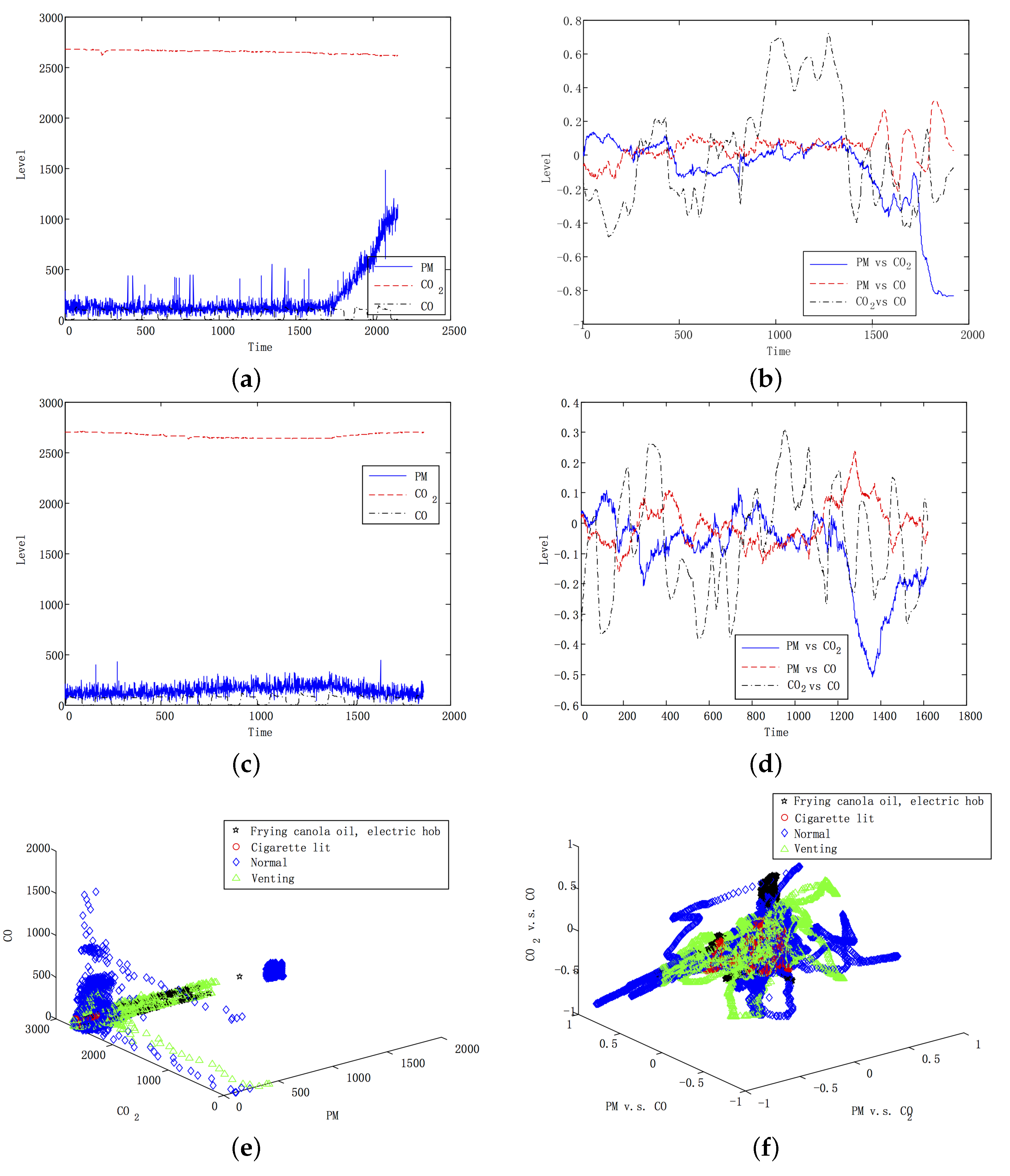
Figure 3 visualizes the pollutants interaction knowledge in terms of its effectiveness for emission sources classification. The left column figures plot the original pollutants level, and the right column figures present the distribution of correlation coefficients from a pair of pollutants. As seen in Figure 3a,c, before data filtering it is very hard to distinguish the two events “Frying canola oil, electric hob” and “Smoking”. In contrast, the right column Figure 3b,d present the data distributions of pollutants interaction represented by correlation coefficients, where the two emission events differences are seen magnified in the pollutants interaction space. In addtion, a 3D data distribution of pollutants levels and pollutants interaction for both observed events with session “Venting” and “Normal” are presented in Figure 3e,f, respectively. It is evident that the discriminant capability of pollutants interaction knowledge is much better than that from the original pollutant levels.

3.2. Accuracy

To conduct the experimentation, the original feature vectors are transformed by the proposed correlation method from an M-dimensional to M ( M 1 ) 2 -dimensional space. The classification accuracy in percentage is obtained from SVM for the M ( M 1 ) 2 dimensional correlation space and M dimensional PCA and LDA spaces, respectively. The performance comparison results are summarized in Table 3. We also report in the table the results when no feature extraction is conducted (denoted as “without data filtering") and with the same SVM classifier applied to get the classification performance. We present the generalization accuracy averaged over 100 trials (denoted as a v e r a g e a c c u r a c y ) and calculate the standard deviation (denoted as s t d e v ) and the accuracy change (denoted as g r o w t h ) when two different sliding windows are applied. As seen from the table, it is evident that the correlation coefficient method is performing much better than the LDA and PCA technique, as well as the case of without data filtering on detecting all seven emission events including (1) frying canola oil on electric hob, (2) frying olive oil on an electric hob, (3) frying olive oil on a gas hob, (4) spray of household pesticide, (5) lighting a cigarette and allowing it to smoulder, (6) no activities, and (7) venting session.

3.3. Sensitivity and Robustness

To verify the sensitivity and performance of the three feature-extraction methods, the accuracy and standard deviations under different sliding window sizes were analysed. In the following, the results of each performance index are demonstrated and discussed in detail.
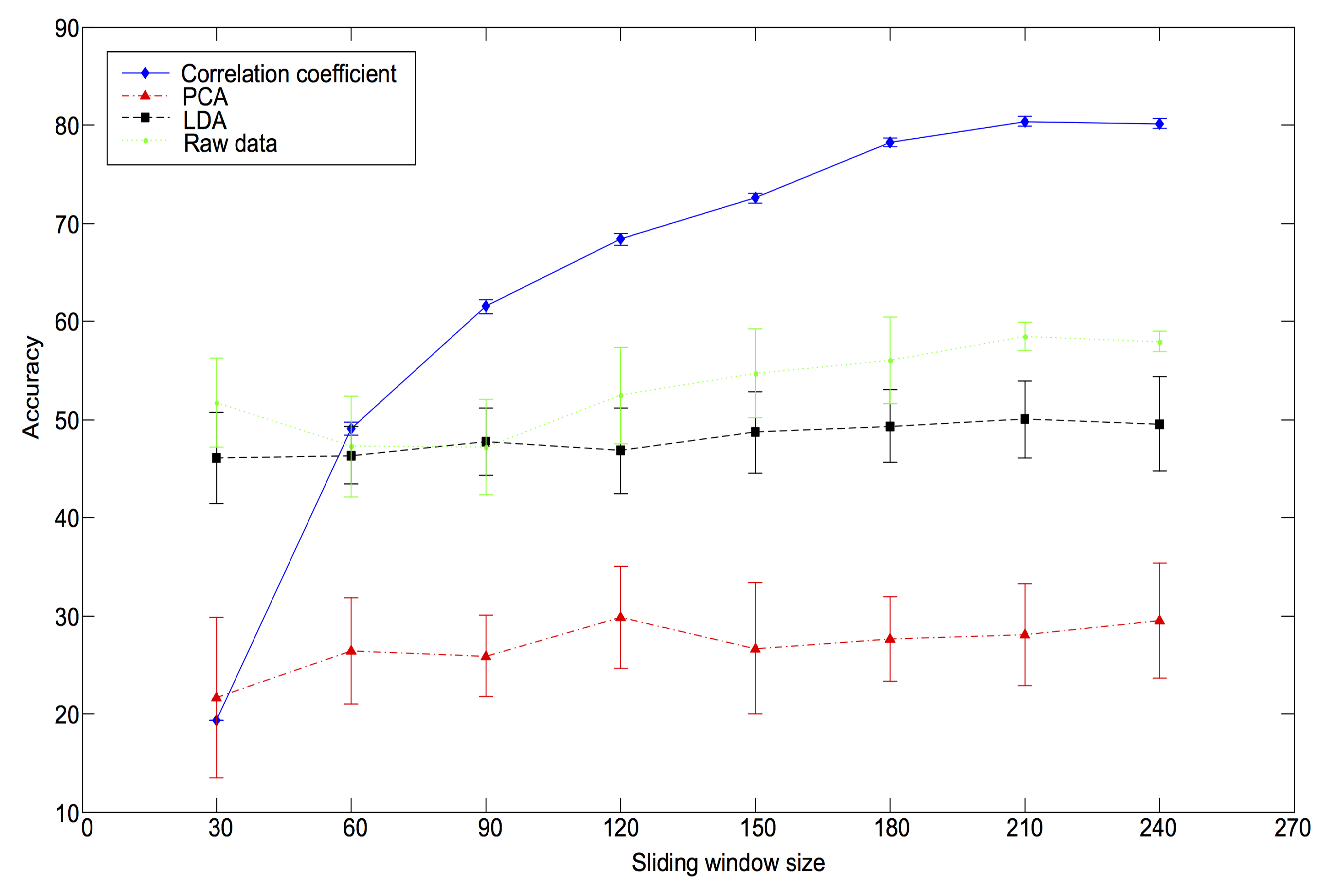
Figure 4 reveals the average accuracy and standard deviation variation under the condition of different sliding window sizes. As seen from the figure, the lowest performance of the proposed method appeared when the sliding window was 30 s. As larger sliding window sizes were imported into the system, the performances of the proposed method rose consistently and finally reached the highest accuracy of 80.35%. In comparison, PCA did not perform as well as the proposed method for any sliding window size greater than 40 s. LDA and without data filtering gave better performances than the proposed method, when the sliding window size was smaller than 60 s. However, all accuracies were less than 60%. The proposed method started to surpass all the other three methods when the sliding window rose to 60 s. When the sliding window increased further to 90 s, the proposed methods accuracy grew to over 60%, while the remaining methods were still in a range below 60%.
Table 4 reports the numerical testing results of the above experiments. As seen from the table, the accuracy grew in general for all methods, and the proposed method received the highest positive growth for most cases. Furthermore, the standard deviations of the proposed method were steady for different sliding window sizes. The largest standard deviation of the proposed method was merely 0.7064%, which was even smaller than the smallest standard deviations from LDA (i.e., 2.9167%), PCA (i.e., 4.1153%) and without data filtering (i.e., 1.0551%). This indicated that the proposed method had outstanding robustness properties, as measured by the standard deviation.

4. Conclusions

In this study, the correlation of pollutants is mathematically calculated for the detection of emission sources in indoor environment. Extensive experiments have confirmed the effectiveness and efficiency of our correlation calculation in real-time detecting emission sources under various experimental settings, which covers seven emission events: (1) frying canola oil on electric hob, (2) frying olive oil on an electric hob, (3) frying olive oil on a gas hob, (4) spray of household pesticide, (5) lighting a cigarette and allowing it to smoulder, (6) no activities, and (7) venting session.
Its worth noting that compared to the case without capturing pollutants interaction data, the detection accuracy of the proposed correlation calculation increases over 20%. It follows that pollutants interaction is indicating a predictive relationship that can be exploited to identify an emission event. The additional information (pollutants correlation) related to the emission sources is necessary and useful for the identification of the emission source in indoor environment.

Author Contributions

Conceptualization, S.P. and G.C.; methodology, S.P. and L.S.; data collection, L.S., I.L. and G.O.; validation, S.P., G.C., I.L. and A.S.; writing—original draft preparation, L.S.; writing—review and editing, S.P. and G.C.; supervision, A.S.; project administration, S.P., G.C. and A.S.; funding acquisition, S.P. and A.S. All authors have read and agreed to the published version of the manuscript.

Funding

This research received no external funding.

Institutional Review Board Statement

Not applicable.

Informed Consent Statement

Not applicable.

Conflicts of Interest

The authors declare no conflict of interest.

References

  1. Gurjar, B.R.; Molina, L.T.; Ojha, C.S.P. Air Pollution: Health and Environmental Impacts; CRC Press: Boca Raton, FL, USA, 2010. [Google Scholar]
  2. Amann, M.; Bertok, I.; Borken-Kleefeld, J.; Cofala, J.; Heyes, C.; Hglund-Isaksson, L.; Klimont, Z.; Nguyen, B.; Posch, M.; Rafaj, P.; et al. Cost-effective control of air quality and greenhouse gases in europe: Modeling and policy applications. Environ. Model. Softw. 2011, 26, 1489–1501. [Google Scholar] [CrossRef]
  3. Bönisch, U.; Böhme, A.; Kohajda, T.; Mögel, I.; Schütze, N.; von Bergen, M.; Simon, J.C.; Lehmann, I.; Polte, T. Volatile organic compounds enhance allergic airway inflammation in an experimental mouse model. PLoS ONE 2012, 7, e39817. [Google Scholar] [CrossRef] [Green Version]
  4. Heinrich, J. Influence of indoor factors in dwellings on the development of childhood asthma. Int. J. Hyg. Environ. Health 2011, 214, 1–25. [Google Scholar] [CrossRef]
  5. Wang, W.; Ramkumar, S.; Li, S.; Wong, D.; Iyer, M.; Sakadjian, B.B.; Statnick, R.M.; Fan, L.-S. Subpilot demonstration of the carbonation- calcination reaction (ccr) process: High-temperature co2 and sulfur capture from coal-fired power plants. Ind. Eng. Chem. Res. 2010, 49, 5094–5101. [Google Scholar] [CrossRef]
  6. Joly, M.; Peuch, V.-H. Objective classification of air quality monitoring sites over europe. Atmos. Environ. 2012, 47, 111–123. [Google Scholar] [CrossRef]
  7. Mas, S.; de Juan, A.; Tauler, R.; Olivieri, A.C.; Escandar, G.M. Application of chemometric methods to environmental analysis of organic pollutants: A review. Talanta 2010, 80, 1052–1067. [Google Scholar] [CrossRef] [PubMed]
  8. Watson, J.G.; Chow, J.C.; Chen, L.-W.A.; Lowenthal, D.H.; Fujita, E.M.; Kuhns, H.D.; Sodeman, D.A.; Campbell, D.E.; Moosmüller, H.; Zhu, D.; et al. Particulate emission factors for mobile fossil fuel and biomass combustion sources. Sci. Total. Environ. 2011, 409, 2384–2396. [Google Scholar] [CrossRef] [PubMed]
  9. Kong, S.; Han, B.; Bai, Z.; Chen, L.; Shi, J.; Xu, Z. Receptor modeling of pm2.5, pm10 and tsp in different seasons and long-range transport analysis at a coastal site of tianjin, china. Sci. Total. Environ. 2010, 408, 4681–4694. [Google Scholar] [CrossRef] [PubMed]
  10. Pacyna, E.G.; Pacyna, J.; Sundseth, K.; Munthe, J.; Kindbom, K.; Wilson, S.; Steenhuisen, F.; Maxson, P. Global emission of mercury to the atmosphere from anthropogenic sources in 2005 and projections to 2020. Atmos. Environ. 2010, 44, 2487–2499. [Google Scholar] [CrossRef]
  11. Wannaz, E.D.; Carreras, H.A.; Rodriguez, J.H.; Pignata, M.L. Use of biomonitors for the identification of heavy metals emission sources. Ecol. Indic. 2012, 20, 163–169. [Google Scholar] [CrossRef]
  12. Cuadros, J.F.; Melo, D.C.; Maciel Filho, R.; Wolf, M.R. Fluid catalytic cracking environmental impact: Factorial design coupled with genetic algorithms to minimize carbon monoxide pollution. Chem. Eng. 2012, 26, 243–248. [Google Scholar]
  13. Fisher, R.A. The use of multiple measurements in taxonomic problems. Ann. Eugen. 1936, 7, 179–188. [Google Scholar] [CrossRef]
  14. Marié, D.C.; Chaparro, M.A.; Gogorza, C.S.; Navas, A.; Sinito, A.M. Vehicle-derived emissions and pollution on the road autovia 2 investigated by rock-magnetic parameters: A case study from argentina. Studia Geophys. Geod. 2010, 54, 135–152. [Google Scholar] [CrossRef] [Green Version]
  15. Blasco, M.; Domeño, C.; López, P.; Nerín, C. Behaviour of different lichen species as biomonitors of air pollution by pahs in natural ecosystems. J. Environ. Monit. 2011, 13, 2588–2596. [Google Scholar] [CrossRef]
  16. Masiol, M.; Squizzato, S.; Ceccato, D.; Rampazzo, G.; Pavoni, B. A chemometric approach to determine local and regional sources of {PM10} and its geochemical composition in a coastal area. Atmos. Environ. 2012, 54, 127–133. [Google Scholar] [CrossRef] [Green Version]
  17. Jolliffe, I.T. Principal Component Analysis; Springer: New York, NY, USA, 1986; Volume 487. [Google Scholar]
  18. Montoya-Mayor, R.; Fernández-Espinosa, A.J.; Ternero-Rodríguez, M. Assessment of the sequential principal component analysis chemometric tool to identify the soluble atmospheric pollutants in rainwater. Anal. Bioanal. Chem. 2011, 399, 2031–2041. [Google Scholar] [CrossRef] [PubMed]
  19. Huang, J.; Choi, H.-D.; Hopke, P.K.; Holsen, T.M. Ambient mercury sources in rochester, ny: Results from principle components analysis (pca) of mercury monitoring network data. Environ. Sci. Technol. 2010, 44, 8441–8445. [Google Scholar] [CrossRef]
  20. Wang, Z.; Luo, P.; Cheng, L.; Zhang, S.; Shen, J. Hapten–antibody recognition studies in competitive immunoassay of α-zearalanol analogs by computational chemistry and pearson correlation analysis. J. Mol. Recognit. 2011, 24, 815–823. [Google Scholar] [CrossRef] [PubMed]
  21. Makarewicz, J.C.; Lewis, T.W.; Boyer, G.L.; Edwards, W.J. The influence of streams on nearshore water chemistry, lake ontario. J. Great Lakes Res. 2012, 38, 62–71. [Google Scholar] [CrossRef]
  22. Rasmussen, D.; Fiore, A.; Naik, V.; Horowitz, L.; McGinnis, S.; Schultz, M. Surface ozone-temperature relationships in the eastern us: A monthly climatology for evaluating chemistry-climate models. Atmos. Environ. 2012, 47, 142–153. [Google Scholar] [CrossRef]
  23. Brudzynski, K.; Miotto, D. The relationship between the content of maillard reaction-like products and bioactivity of canadian honeys. Food Chem. 2011, 124, 869–874. [Google Scholar] [CrossRef]
  24. Olivares, G.; Longley, I.; Coulson, G. Development of a low-cost device for observing indoor particle levels associated with source activities in the home. In Technical Report, NIWA New Zealand; International Society of Exposure Science (ISES): Seattle, WA, USA, 2012. [Google Scholar]
  25. Hearst, M.A. Support vector machines. IEEE Intell. Syst. 1998, 13, 18–28. [Google Scholar] [CrossRef] [Green Version]
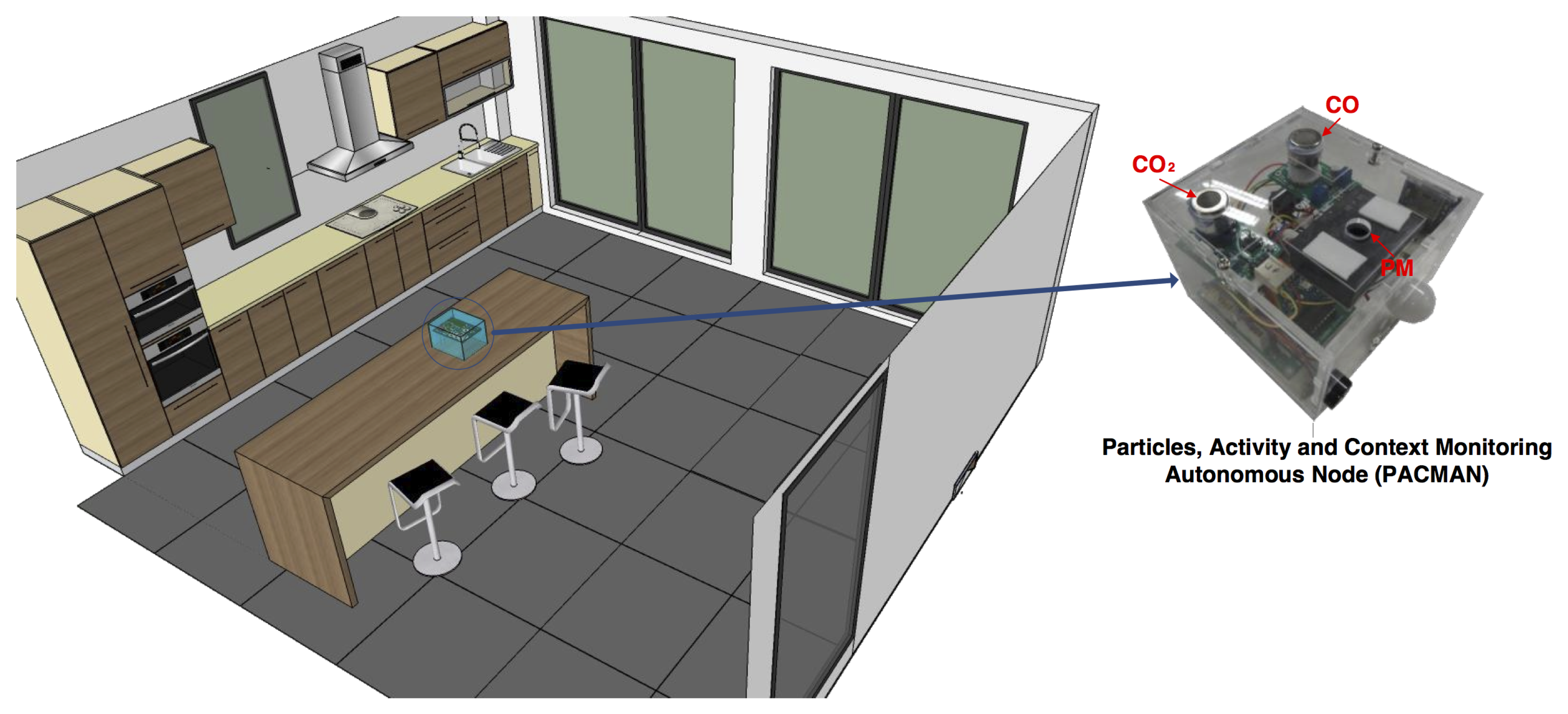
Figure 1. The experimental environment.
Applsci 11 07542 g001
Figure 2. Data sequences X with length T, the subsequence of length w = 120 and the subsequences extracted by a sliding window c. Note that the sliding windows overlap.
Applsci 11 07542 g002
Figure 3. (a) Levels of contaminants obtained from PACMAN for event “frying canola oil, electric hob”; (b) deterministic components obtained after data filtering for event “frying canola oil, electric hob” (c) levels of contaminants obtained from PACMAN for event “smoking”; (d) deterministic components obtained after data filtering “smoking”; (e) the native organization of contaminants for the two events with sessions “venting” and “normal” distributed in 3D space; (f) the filtered data for the two events with sessions “venting” and “normal” distributed in 3D space.
Applsci 11 07542 g003
Figure 4. The performance variation of target-feature-extraction methods under the condition of different sliding window sizes.
Applsci 11 07542 g004
Table 1. Summary of the measured parameters and sensors in the PACMAN units.
ParameterSensorNotes
Carbon monoxide (CO)Hanwei MQ-772 h warm-up period
90 s time resolution
Carbon dioxide (CO 2 )Hanwei MG-8112 h warm-up period
Temperature (T)LM335AMeasuring temperature
outside the enclosure
Movement (M)PIR60 field-of-view
Distance (d)Maxbotix range finder6.5 m range
Particulate Matter ( P M 10 )Dust sensorbaseline offset 1500 mV
Table 2. A summary of the notation used in this paper.
X R T × M The basic data structure, which can cover a majority of the indoor conditions
tThe index of the time point
TTotal elapsed time
x ( t ) R 1 × M Samples at time t
wThe size of the sliding window
MThe total number of observed pollutants
mThe index of the pollutant
N = T w + 1 The total number of subsequences
iThe index of the sliding window
CA set of matrices extracted by slicing time series with sliding window w
c i R w × M An extracted subsequence from the ith sliding window
r i , j , k The correlation coefficient of two pollutants (i.e., jth and kth) for the ith sliding window
Table 3. A comparison of the algorithms using classification accuracy in percentage as a prototype for the events (1) frying canola oil on an electric hob, (2) frying olive oil on an electric hob, (3) frying olive oil on a gas hob, (4) spraying of household pesticide, (5) lighting a cigarette and allowing it to smoulder, (6) no activities and (7) venting session.
Correlation CoefficientPCA
AccuracyConfusion MatrixAccuracyConfusion Matrix
80.14%class123456729.49%class1234567
1305.449.720.200.443.8411.4837.521155.4419.680.242.5265.7629.3695.64
216.76484.280.920.164.1621.44151.96218.80344.6057.080.1227.4064.64167.04
30.201.32387.121.360.242.6010.3631.36150.7291.520.1226.4846.6886.32
40.3200.52125.160.200.160.36430.6021.0015.168.40013.9237.64
58.3614.080.840.52188.0811.1288.04526.0019.524.360.04210.007.0044.12
616.1638.962.680.4013.32773.24170.926134.92348.6484.406.3659.52126.28255.56
725.3657.926.240.3626.6062.441882.207388.96295.96282.0411.68233.52259.52589.44
LDAWithout data filtering
AccuracyConfusion matrixAccuracyConfusion matrix
49.54%class123456757.95%class1234567
13.761.20002.8824.92335.88157.005.48000.680.92304.56
22.96304.44012.201.4013.16345.5221.08580.64000.8436.2460.88
30.280343.60000.0459.28300403.200000
400.76017.2400108.7245.0800100.160021.48
58.960.00005.2439.40257.44500.04007.441.64301.92
627.9616.8825.08023.52273.44648.80631.2475.882.52037.84381.40486.80
737.2061.4438.7632.6048.92227.281614.92762.72139.08110.60100.0892.2488.481467.92
Table 4. Comparison of four feature extractions under the condition of different sliding window sizes.
Feature Extraction MethodThe Sliding Window Size
306090120150180210240
Correlation coefficientaverage accuracy19.32%49.06%61.50 %68.36%72.59%78.19%80.35%80.14%
growth-29.74%12.44 %6.86 %4.23 %5.60%2.17%−0.21 %
stdev0.00010.61850.70640.61700.49450.43580.49060.4958
LDAaverage accuracy46.06%46.32 %47.77%46.81%48.70%49.32%50.01%49.54%
growth-0.26%1.45%−0.96%1.89%0.63%0.69%−0.47%
stdev4.62162.91673.40964.34714.11563.67753.92704.7798
PCAaverage accuracy21.61%26.44%25.91%29.82%26.68%27.63%28.07%29.49%
growth-4.83%−0.53%3.92%−3.15%0.96%0.44%1.42%
stdev8.17035.42144.11535.19706.64874.35475.16035.8455
Without data filteringaverage accuracy51.74%47.27%47.17%52.45%54.69%56.01%58.47%57.95%
growth-−4.47%−0.10 %5.28%2.24%1.33%2.45%−0.52%
stdev4.52545.15154.82874.954.55944.38401.46201.0551
Publisher’s Note: MDPI stays neutral with regard to jurisdictional claims in published maps and institutional affiliations.