About the Use of Generalized Forms of Derivatives in the Study of Electromagnetic Problems

Abstract

The use of non-local operators, defining Riemann–Liouville or Caputo derivatives, is a very useful tool to study problems involving non-conventional diffusion problems. The case of electric circuits, ruled by non-integer derivatives or capacitors with fractional dielectric permittivity, is a fairly natural frame of relevant applications. We use techniques, involving generalized exponential operators, to obtain suitable solutions for this type of problems and eventually discuss specific problems in applications.

1. Introduction

The use of non-integer and integral operators [1,2,3,4,5,6] has evolved into the Differ-Integral Calculus (DIC). The mathematical environment in which DIC has grown is that of the generalized transform. Most of the associated concepts are well framed within the context of appropriate integral transforms [2,7]. The techniques associated with the DIC, combined with other methods of operational nature, has provided significant progress within the context of applied mathematics in general and of applied classical electromagnetic field theory in particular and the relevant roots can be traced back to the original works of Heaviside [8].

The associated technicalities have played, in the past, important roles in the study of equations describing evolution problems in relativistic Quantum Mechanics and tracing back to the work of Klein Gordon and Dirac [9]. Within this context, an important step has been the understanding of the role played of DIC within the most general framework of pseudo and non-local operator theory [10,11,12,13]. The most natural context for the study of differential equations, be they of ordinary or partial nature, is the use of techniques tracing back to the evolution operator and to generalized integral transforms, including those of Lévy-type [14]. We will provide a description of these methods by reviewing a number of applications of what is defined as (in a broad sense) fractional calculus.

An application field where fractional calculus has received an increasing attention over the years is CMOS-based applications. According to the International Technology Roadmap for Semiconductors (ITRS), the expected cut-off frequency of CMOS transistors is 0.9 THz in 2021. At such high frequencies, the primary challenge in CMOS-based THz design is to develop accurate device models that allow one to take the loss from strong frequency-dependent dispersion and non quasi-static effects in THz into account. Traditionally, on-chip interconnects are characterized by the distributed integer order RLGC model. Drude’s classical relaxation-effect model is used for the skin effect modeling [15]. In addition, the loss due to dielectric polarization and dipole rotation can be modeled by a dielectric-loss still using integer-order models. However, such an integer-order model is insufficient to describe the transmission line performance at the THz region because the loss term in transmission line theory is difficult to model the dispersion loss and non-quasi-static effects [16] which may cause a large deviation in the THz frequency region. Some valuable models of fractional-order models of transmission lines are presented in [17,18].

A generalization of the CMOS circuit driving a distributed fractional RLC load into the fractional-order domain has been presented in [19], making the on-chip interconnect structure easy to adjust by including the effect of the fractional orders. Hence, incorporation of fractional-order models becomes crucial to properly address both electromagnetic compatibility as well as signal integrity issues.

Another field where fractional-order models have become important is that of pulsed electric fields (PEFs). The main goal of this discipline is the study of the interaction between biological tissues and electromagnetic fields aiming at the investigation of the use of ultrashort pulses in biomedical applications [20]. It is known that the electric field distribution excited in biological media mainly depends on the electric properties of tissues. The dielectric properties of biological tissues result from the interaction of electromagnetic energy with the tissue constituents at the cellular and molecular level which is strongly affected by the bound water content. The dielectric properties of many biological materials exhibit an experimental dielectric response in the frequency domain that cannot be described by a simple exponential expression with a single relaxation time (Debye model). On the contrary, empirical fractional-order relationships including Cole–Cole (C–C), Cole–Davidson (C–D), and Havriliak––Negami (H–N) equations have been proposed in order to fit such dielectric spectra. The evaluation of the transient propagation of electromagnetic waves in these types of fractional-order dielectric media is not trivial since it contains the transformation of the fractional-order expressions from the frequency domain to the time-domain. It has been addressed in the context of the finite different time-domain (FDTD) method by resorting to the auxiliary differential equation (ADE) approach [21,22]. An alternative approach based on the application of the Riemann–Liouville theory to the analysis of C–C media has been proposed in [23,24]. The double fractional derivative operator relevant to the general H–N response is directly incorporated in the FDTD basic algorithm in [25].

What we would like to convey here is the strong interplay between DIC and integral transforms. They constitute the relevant backbone and probably the intimate mathematical flavor. The paper is therefore planned as follows.

In Section 2 we show how the concept of fractional integral emerges from the study of the Lamb–Bateman integral equation. The emergency of the Liouville–Riemann definition of fractional derivative is then shown to naturally emerge from the Laplace transform, which is then exploited to treat fractional ODE’s.

The rest of the papers deal with specific applications of “fractional” electric circuits and extension to RC circuits with non-standard permittivity.

Finally, we go back to quantum-like models by treating the case of relativistic heat equations.

2. Lamb-Bateman Equation, Operational Methods, and Fractional Calculus

We give an idea of the underlying technicalities, also exploited in this article, by discussing the solution of the Lamb–Bateman equation [26,27,28].

Example 1.

The Lamb–Bateman equation, originally proposed for the solution of a solitary wave, is written as

$${\int }_0^{\infty }u(x-y^2)dy=f(x)$$

(1)

where $u(x)$ is a function to be determined in terms of $f(x)$. The relevant solution is readily achieved by the use of operational methods [29], allowing one to recast it in the form

$$\hat{L} u(x)=f(x),\hspace{1em}\hspace{1em}\hspace{1em}\hat{L}={\int }_0^{\infty }{e}^{-y^2{\partial }_x}dy ,$$

(2)

which is just a consequence of the shift operator identity [29]

$$e^{a{\partial }_x}f(x)=f(x+a).$$

(3)

If we take the freedom of treating the derivative operator, in the definition of $\hat{L}$, as an ordinary algebraic quantity, we can work out the Gaussian integral and end up with the explicit definition of the operator $\hat{L}$ as

$$\hat{L}=\frac{1}{2}\sqrt{\frac{\pi }{{\hspace{1em}}_x}},$$

(4)

thus obtaining

$${\hat{L}}^{-1}=\frac{2}{\sqrt{\pi }} {{\partial }_x}^{\frac{1}{2}}$$

(5)

and eventually

$$u(x)=\frac{2}{\sqrt{\pi }}{{\partial }_x}^{\frac{1}{2}}f(x).$$

(6)

We accordingly expressed the solution of the Lamb–Bateman equation in terms of the derivative of order $\frac{1}{2}$ of the function $f(x)$.

The next step is that of stipulating the action of a fractional derivative on a given function.

Exercise 1.

We recall first the Laplace transform identity

$$a^{-\nu }=\frac{1}{\Gamma (\nu )}{\int }_0^{\infty }{e}^{-as}{s}^{\nu -1}ds,\hspace{1em}\hspace{1em}Re(a),Re(\nu )>0 ,$$

(7)

which, by using Equation (3), allows writing of the following

$${\partial }_x^{-\frac{1}{2}}g(x)=\frac{1}{\Gamma \left(\frac{1}{2}\right)}{\int }_0^{\infty }{e}^{-s{\partial }_x}{s}^{-\frac{1}{2}}ds g(x)=\frac{1}{\Gamma \left(\frac{1}{2}\right)}{\int }_0^{\infty }{s}^{-\frac{1}{2}}g(x-s)ds.$$

(8)

Changing the integration variable and arranging the limits of integration, we eventually find

$${}_a{\partial }_x^{-\frac{1}{2}}g(x)=\frac{1}{\sqrt{\pi }}{\int }_a^x{(x-\xi )}^{-\frac{1}{2}}g(\xi )d\xi .$$

(9)

The lowest integration limit, following from (8), is $-\infty$; we put a generic a to be consistent with the current definition of the differintegral operator. If $a=0$ the sub-index on the left of the derivative operator will be neglected. The use of the semigroup property of the fractional differintegral operator [1,2,3,4,5,6]

$${{\partial }_x}^{\frac{1}{2}}={\partial }_x^{-\frac{1}{2}}{\partial }_x$$

(10)

finally leads to

$${{\partial }_x}^{\frac{1}{2}}g(x)=\frac{1}{\sqrt{\pi }}{\int }_0^x{(x-\xi )}^{-\frac{1}{2}}{g}^{\prime }(\xi )d\xi .$$

(11)

The apex in front of $g(x)$ denotes first-order derivative.

In the previous Exercise, we adopted 0 as the lower limit. The relevant value should however be chosen in agreement with the specific problem under study. Further comments will be provided in the final comments.

Remark 1.

More in general, any derivative of order$\alpha$can be written as

$${\partial }_x^{\alpha } g(x)={\partial }_x^{(\alpha -1)}{g}^{\prime }(x)=\frac{1}{\Gamma (1-\alpha )}{\int }_0^x{(x-\xi )}^{-\alpha }{g}^{\prime }(\xi )d\xi ,\hspace{1em}\hspace{1em}0<\alpha <1,$$

(12)

which is the definition of the fractional derivative according to Caputo [30,31]. Equation (12) states, with the ordinary derivative, that the fractional derivative of a constant is vanishing. This feature is not contained in other forms of fractional derivatives (e.g., the Riemann–Liouville and Euler derivatives [1,2,3,4,5,6]).

In the following, we limit ourselves to the derivative order with $0<\alpha <1$ and just touch on the cases with $\alpha >1$ later in the article.

The Caputo derivative (as well as the others) is a non-local integral operator, not dissimilar from those entering the treatment of pseudo-differential operators in relativistic quantum mechanic [9,10,11,13,32,33].

Observation 1.

Regarding the use of this family of operators we note, e.g., that the solution of non-homogeneous differential equation

$${(\alpha -{\hat{D}}_x)}^{\nu }y(x)=f(x),$$

(13)

where $y(x)$ is the unknown, can be formally written as

$$y(x)=\frac{1}{{\left(\alpha -{\hat{D}}_x\right)}^{\nu }}f(x).$$

(14)

The use of the Laplace transform identity applied to the operator

$$\frac{1}{{(\alpha -{\hat{D}}_x)}^{\nu }}=\frac{1}{\Gamma (\nu )}{\int }_0^{\infty }{\xi }^{n-1}{e}^{-\left(a-{\hat{D}}_x\right)\xi }d\xi$$

(15)

and of the exponential shift operator (3) yields

$$y(x)=\frac{1}{\Gamma (\nu )}{\int }_0^{\infty }{\xi }^{n-1}{e}^{-a\xi }f(x+\xi )d\xi .$$

(16)

By exploiting Observation 1 we can provide the solution to the following problem involving partial fractional derivatives.

Problem 1 (Heat-like Equation).

The solution of evolution-like equations involving partial fractional derivatives as, e.g.,

$$\left\{\begin{array}{c}\frac{\partial }{\partial t}F(x,t)=-\frac{{\partial }^{\alpha }}{\partial x^{\alpha }}F(x,t)\hfill \\ {\left.F(x,t)\right|}_{t=0}=f(x),\hspace{1em}\hspace{1em}0<\alpha <1\hfill \end{array}\right.$$

(17)

can be viewed as a kind of heat equation [13,29,34,35,36] and solved by the use of an appropriate transform. The use of the formalism of the evolution operator [29,37] yields

$$F(x,t):=F_{\alpha }(x,t)={\hat{U}}_{\alpha }(t)f(x),\hspace{1em}\hspace{1em}\hspace{1em}\hspace{1em}{\hat{U}}_{\alpha }(t)=e^{-t\frac{{\partial }^{\alpha }}{\partial x^{\alpha }}}.$$

(18)

The action of the evolution operator $\hat{U}(t)$ on the initial function $\gamma (x)$ can be obtained via the so-called Lévy transform method [13,14]. To this aim, we note that the following integral transform, concerning the stretching integral, is known as one-sided Lévy stable distribution (Equation (19) is also known as Kohlrausch–Williams–Watts function [38].) $g_{\gamma }(\eta )$ [14] and acts in the following way

$$e^{-\tau x^{\gamma }}={\int }_0^{\infty }{e}^{-{(\tau x^{\gamma })}^{{\gamma }^{-1}}\eta } g_{\gamma }(\eta ) d\eta ={\int }_0^{\infty }{e}^{-{\tau }^{{\gamma }^{-1}}x \eta } g_{\gamma }(\eta ) d\eta ,\hspace{1em}\forall \gamma ,x,\tau \in \mathbb{R}:0<\gamma <1,\hspace{1em}x,\tau >0.$$

(19)

We can therefore manage to transform the exponential evolution operator in Equation (18) as

$${\hat{U}}_{\alpha }(t)={\int }_0^{\infty }{e}^{-t^{{\alpha }^{-1}}\eta \frac{\partial }{\partial x}}{g}_{\alpha }(\eta )d\eta ,$$

(20)

which eventually yields, for the solution of our problem,

$$F_{\alpha }(x,t)={\int }_0^{\infty }{g}_{\alpha }(\eta )f\left(x-t^{{\alpha }^{-1}}\eta \right)d\eta .$$

(21)

Other forms of fractional derivatives have appeared in the literature.

Remark 2.

If, in Equation (21), we consider the case with$\alpha =\frac{1}{2}$, the Lévy distribution writes

$$g_{\frac{1}{2}}(\eta )=\frac{1}{2\sqrt{\pi } {\eta }^{\frac{3}{2}}}{e}^{-\frac{1}{4\eta }}$$

(22)

which, for an initial Gaussian distribution, yields the temporal behaviour reported in Figure 1 which displays the interesting feature that, while time increases, the initial gaussian distribution develops the long tail shape characteristic of a Lévy distribution.

Figure 1. Solution $F(x,t)$ of Equation (21) at different times t, for $\alpha =\frac{1}{2}$ and initial function $f(.)$ being a Gaussian.

The same procedure can be applied when dealing with slightly more complicated problems, like in the following problem.

Problem 2.

Let,$\forall x\in \mathbb{R}$,$\forall t\in {\mathbb{R}}^{+}$

$$\left\{\begin{array}{c}{\partial }_{t}F(x,t)=-\sqrt{1+{\partial }_x^{\nu }} F(x,t),\hfill \\ F(x,0)=f(x)\hfill \end{array}\right.$$

(23)

whose formal solution reads

$$F(x,t):=F_{\nu }(x,t)=e^{-t\sqrt{1+{\partial }_x^{\nu }}}f(x).$$

(24)

Explicitly, in terms of the Lévy functions $g_{\frac{1}{2}}(\eta )$, according to Equation (19) we find

$$\begin{array}{cc}\hfill F_{\nu }(x,t)& ={\int }_0^{\infty }{e}^{-t^2\left(1+{\partial }_x^{\nu }\right)\eta }{g}_{\frac{1}{2}}(\eta )d\eta f(x)={\int }_0^{\infty }{g}_{\frac{1}{2}}(\eta )e^{-\eta t^2}\left({\int }_0^{\infty }{e}^{-{\left(\eta t^2\right)}^{\frac{1}{\nu }}{\partial }_x \epsilon }{g}_{\nu }(\epsilon )d\epsilon f(x)\right)d\eta =\hfill \\ & ={\int }_0^{\infty }{g}_{\frac{1}{2}}(\eta )e^{-\eta t^2}\left({\int }_0^{\infty }{g}_{\nu }(\epsilon )f\left(x-{\left(\eta t^2\right)}^{\frac{1}{\nu }}\epsilon \right)d\epsilon \right)d\eta .\hfill \end{array}$$

(25)

In Figure 2 we reported a comparison between the solutions of the fractional PDE in (17) and in (23) for $\nu =\frac{1}{2}$. They are qualitatively similar; they exhibit the development of an asymmetric long tail for increasing time, with a significantly larger reduction in the peaks in the case (23).

Figure 2. Comparison between the solutions of Equations (17) and (23) for $v=\frac{1}{2}$ and different values of t. (a) t = 0.5; (b) t = 1.

An analogous technique has been discussed in Ref. [13], where a generalized form of the heat equation ($\alpha =2$) has been considered in terms of a double transformation (Lévy & Gauss–Weierstrass).

Remark 3.

In order to obtain a more complete picture of the formalism we have foreseen, we consider the solution of Equation (23) for the cases with$\alpha =\frac{1}{3}$and$\alpha =\frac{2}{3}$. To this aim, we remind that [39,40]

$$g_{\frac{1}{3}}(\eta )=\frac{1}{3\pi }\frac{K_{\frac{1}{3}}\left(\frac{2}{3\sqrt{3 \eta }}\right)}{\sqrt{{\eta }^3}},\hspace{1em}\eta \ge 0,\hspace{1em}\hspace{1em}\hspace{1em}{K}_{\alpha }(x)=\frac{1}{2}{\left(\frac{x}{2}\right)}^{\alpha }{\int }_0^{\infty }{e}^{-t-\frac{x^2}{4t}} t^{-p-1}dt$$

(26)

with$K_{\alpha }(x)$being the second kind modified Bessel function and

$$\begin{array}{c}{g}_{\frac{2}{3}}(\eta )=\sqrt{\frac{3}{\pi }} {\displaystyle \frac{e^{-\frac{y}{2}}}{\eta }}{W}^{\left(\frac{1}{2},\frac{1}{6}\right)}(y),\hspace{1em}\hspace{1em}\hspace{1em}\hspace{1em}y=\frac{4}{27{\eta }^2},\hfill \\ W^{(\kappa ,\mu )}(x)=e^{-\frac{x}{2}}{x}^{\mu +\frac{1}{2}}U\left(\mu -\kappa +\frac{1}{2},2\mu +1;x\right),\hfill \\ U(a,c;x)=\frac{1}{\Gamma (a)}{\int }_0^{\infty }{e}^{-xt}{t}^{a-1}{(1+t)}^{c-a-1}dt,\hspace{1em}\hspace{1em}\hspace{1em}Re(a)>0,\hfill \end{array}$$

(27)

where$W^{(\kappa ,\mu )}(x)$is the Whittaker function and$U(a,c;x)$the confluent hyper-geometric function of the second kind. The comparison between the solution of Equation (23) with$\alpha =\frac{1}{3},\frac{2}{3}$is eventually reported in Figure 3.

Figure 3. Comparison between the solutions of Equation (17) for different values of α and t. (a) t = 0.5; (b) t = 1.

As a further example of application of the composite transform method, we consider the solution of the problem given below.

Example 2.

Let, $\forall \nu ,\beta \in \mathbb{R}:0<\nu <1$ and $\beta >0$

$${\hat{D}}_x^{(\nu ,\beta )} u(x)=f(x),\hspace{1em}\hspace{1em}\hspace{1em}{\hat{D}}_x^{(\nu ,\beta )}={(1+{\partial }_x^{\nu })}^{\beta },$$

(28)

where the unknown function $u(x)$ is expressed in terms of $f(x)$ as

$$\begin{array}{cc}\hfill u(x):& =u_{(\nu ,\beta )}(x)={\hat{D}}_x^{(\nu ,-\beta )}f(x)=\frac{1}{\Gamma (\beta )}{\int }_0^{\infty }{e}^{-s}{s}^{\beta -1}{e}^{-s{\partial }_x^{\nu }}ds f(x)=\hfill \\ & =\frac{1}{\Gamma (\beta )}{\int }_0^{\infty }{e}^{-s}{s}^{\beta -1}\left({\int }_0^{\infty }{g}_{\nu }(\eta )f\left(x-\eta s^{{\nu }^{-1}}\right)d\eta \right)ds.\hfill \end{array}$$

(29)

In the following Figure 4, Figure 5 and Figure 6 we provide the functions $u(x)$ for different values of β and ν and $f(x)$ being Gaussian or super-Gaussian function.

Figure 4. Equation (29) for different values of β, $v=\frac{1}{2}$ and f(x) Gaussian or super-Gaussian function. (a) $f(x)=e^{{-x}^2}$ (b) $f(x)=e^{{-x}^4}$.

Figure 5. Equation (29) for different values of β, $v=\frac{1}{3}$ and f(x) Gaussian or super-Gaussian function. (a) $f(x)=e^{{-x}^2}$ (b) $f(x)=e^{{-x}^4}$.

Figure 6. Equation (29) for different values of β, $v=\frac{2}{3}$ and f(x) Gaussian or super-Gaussian function. (a) $f(x)=e^{{-x}^2}$ (b) $f(x)=e^{{-x}^8}$.

Observation 2.

Before concluding this introductory section, we note that for $0<\beta <1$, we can obtain the solution of the Example 2 in alternative way. We consider the fractional differential equation

$${\hat{D}}_x^{(\nu ,-\beta )} u(x)=f(x)$$

(30)

and recast it according to the following

$$\begin{array}{c}{u}_{(\nu ,-\beta )}(x)={\hat{D}}_x^{(\nu ,\beta )} f(x)={\hat{D}}_x^{(\nu ,-(1-\beta ))}{\hat{D}}_x^{(\nu ,1)}f(x)=\frac{1}{\Gamma (1-\beta )}{\int }_0^{\infty }{e}^{-s}{s}^{-\beta }{e}^{-s{\partial }_x^{\nu }}\kappa (x)ds,\hfill \\ \kappa (x)=\left(1+{\partial }_x^{\nu }\right)f(x)\hfill \end{array}$$

(31)

where the action of the fractional exponential operator on the function $\kappa (x)$ can be specified as

$$e^{-s{\partial }_x^{\nu }}\kappa (x)={\int }_0^{\infty }{g}_{\nu }(\eta )\left[f\left(x-\eta s^{{\nu }^{-1}}\right)+f^{(\nu )}\left(x-\eta s^{{\nu }^{-1}}\right)\right]d\eta ,\hspace{1em}\hspace{1em}\hspace{1em}{u}^{(\nu )}(x)={\partial }_x^{\nu }u(x).$$

(32)

It is worth stressing that the use of Equation (12)

$$f^{(\nu )}\left(x-\eta s^{{\nu }^{-1}}\right)={\displaystyle \frac{1}{\Gamma (1-\nu )}}{\int }_0^{x-\eta s^{{\nu }^{-1}}}{\left(x-\xi -\eta s^{{\nu }^{-1}}\right)}^{-\nu }{f}^{\prime }(\xi )d\xi$$

(33)

eventually yields

$$\begin{array}{cc}\hfill e^{-s{\partial }_x^{\nu }}\left({\partial }_x^{\nu }f(x)\right)& =\frac{1}{\Gamma (1-\nu )}{\int }_0^{\infty }{g}_{\nu }(\eta ){\int }_0^{x-\eta s^{{\nu }^{-1}}}{\left(x-\xi -\eta s^{{\nu }^{-1}}\right)}^{-\nu }{f}^{\prime }(\xi )d\xi d\eta =\hfill \\ & ={\int }_0^{\infty }{g}_{\nu }(\eta )f^{(\nu )}\left(x-\eta s^{{\nu }^{-1}}\right)d\eta .\hfill \end{array}$$

(34)

The numerical computation of Equation (31) is accordingly complicated by the necessity of evaluating three nested integrals

$$\begin{array}{cc}\hfill u_{(\nu ,-\beta )}& =\frac{1}{\Gamma (1-\beta )}{\int }_0^{\infty }{e}^{-s}{s}^{-\beta }\left\{{\int }_0^{\infty }{g}_{\nu }(\eta )\left[f\left(x-\eta s^{{\nu }^{-1}}\right)+\right.\right.\hfill \\ & +\left.\left.\left(\frac{1}{\Gamma (1-\nu )}{\int }_0^{x-\eta s^{{\nu }^{-1}}}{\left(x-\xi -\eta s^{{\nu }^{-1}}\right)}^{-\nu }{f}^{\prime }(\xi )d\xi \right)\right]d\eta \right\}ds\hfill \end{array}$$

(35)

or four integrals if we consider the alternative following calculation

$$\begin{array}{cc}\hfill {\hat{D}}_x^{(\nu ,\beta )} u(x)& ={\hat{D}}_x^{(\nu ,-(1-\beta ))}{\hat{D}}_x^{(\nu ,1)}u(x)=f(x)\hspace{1em}\Rightarrow \hfill \\ \hfill \Rightarrow \hspace{1em}u(x)& ={\hat{D}}_x^{(\nu ,(1-\beta ))}{\hat{D}}_x^{(\nu ,-1)}f(x)=\frac{1}{\Gamma (\beta -1)}{\int }_0^{\infty }{e}^{-s}{s}^{\beta -2}{e}^{-s{\partial }_x^{\nu }}\kappa (x)ds=\hfill \\ & =\frac{1}{\Gamma (\beta -1)}{\int }_0^{\infty }{e}^{-s}{s}^{\beta -2}\left({\int }_0^{\infty }{g}_{\nu }(\xi )\kappa \left(x-\xi s^{{\nu }^{-1}}\right)d\xi \right)ds,\hfill \\ \hfill \kappa (x)& ={\hat{D}}_x^{(\nu ,-1)}f(x)={(1+{\partial }_x^{\nu })}^{-1}f(x)={\int }_0^{\infty }{e}^{-k}{e}^{-k{\partial }_x^{\nu }}f(x) dk=\hfill \\ & ={\int }_0^{\infty }{e}^{-k}\left({\int }_0^{\infty }{g}_{\nu }(\eta )f\left(x-\eta k^{{\nu }^{-1}}\right)d\eta \right)dk\hfill \end{array}$$

(36)

and finally

$$u_{(\nu ,\beta )}(x)=\frac{1}{\Gamma (\beta -1)}{\int }_0^{\infty }{e}^{-s}{s}^{\beta -2}\left({\int }_0^{\infty }{g}_{\nu }(\xi )\left({\int }_0^{\infty }{e}^{-k}\left({\int }_0^{\infty }{g}_{\nu }(\eta )f\left(x-\xi s^{{\nu }^{-1}}-\eta k^{{\nu }^{-1}}\right)d\eta \right)dk\right)d\xi \right)ds.$$

(37)

The quadrupole integral on the right is a caveat on the slowness of the associated numerical procedure. Further comments on the subject will be however provided in the concluding section.

3. Generalized Exponential Operators and Fractional Electrical Circuit

In this section, we consider the extension to the fractional case of the differential equations characterizing an electric circuit.

In the previous section we fixed the few elements of the formalism we will use in the following. We privileged, in our definition of fractional derivative, the Caputo form. The reason for this choice stems from the fact that we prefer to avoid ambiguity due to the non-vanishing of the derivative of a constant.

The modeling of an electrical circuit in terms of non-integer differential equations does not appear, in general, well motivated and often the mathematical formalism is privileged with respect to the effective physical meaning. It should be however noted that the Ohm law is at the basis of the circuital phenomena. This law summarizes, from a macroscopic point of view, the microscopic dynamic of charge carriers inside a conductor, along with the relevant interactions defining the charge drift velocity. Classical Newtonian mechanics is used to provide a link between the applied electric field and charge velocities, whereas the diffusion process may be governed by other mechanisms not strictly associated with classical diffusion and more similar to Lévy type process which, according to the discussion of the previous section, requires fractional heat type equations.

We assume, for the moment, that the fractional derivative can model an actual physical circuit and discuss some aspects of the relevant study, in terms of the solutions of the associated differential equations.

Example 3 (RC Circuit).

An ordinary RC circuit is ruled by the first-order differential equation

$$\left\{\begin{array}{c}R\frac{d}{dt}q(t)+\frac{1}{C}q(t)=V(t)\hfill \\ V(t)=V_{0}f(t)\hfill \end{array}\right..$$

(38)

Equation (38), in non dimensional form, gives

$$\frac{d}{d\eta }Q(\eta )+Q(\eta )=f^{*}(\eta ),\hspace{1em}\hspace{1em}\eta =\frac{t}{\tau },\hspace{1em}\hspace{1em}\tau =RC,\hspace{1em}\hspace{1em}Q(\eta )=\frac{q(t)}{C{V}_0},\hspace{1em}\hspace{1em}{f}^{*}(\eta )=f(\tau \eta ).$$

(39)

The non-homogeneous part of the solution can, according to the methods outlined in the previous section, be written as

$$Q(\eta )=\frac{1}{1+{\partial }_{\eta }}{f}^{*}(\eta )={\int }_0^{\infty }{e}^{-s}{e}^{-s{\partial }_{\eta }}{f}^{*}(\eta )ds={\int }_0^{\infty }{e}^{-s}{f}^{*}(\eta -s)ds$$

(40)

and a graphical example is reported in Figure 7a, for $f(\eta )=\cos (\sigma \eta )$, $\sigma =\omega \tau$. The solution was checked numerically to be sure that it is consistent with the original Equation (38).

Figure 7. Solutions of RC circuit (38) in ordinary and fractional cases with initial function f(.) = cos(.). (a) Potential across the capacitor (40) (Q(t)) and external potential (V(t)); (b) Fractional case for potential across the capacitor (Π(t)) for different values of γ.

Before proceeding further it should, however, be noted that, by standard means, the solution of first-order non-homogeneous ODE’s of the type (39) gives

$$Q(\eta ,{\eta }_0)=Q^{*}{e}^{-(\eta -{\eta }_0)}+{\int }_{{\eta }_0}^{\eta }{e}^{-(\eta -\xi )}f(\xi )d\xi$$

(41)

or, after rearranging the integration variable,

$$Q(\eta ,{\eta }_0)=Q^{*}{e}^{-(\eta -{\eta }_0)}+{\int }_0^{\eta -{\eta }_0}{e}^{-\sigma }f(\eta -\sigma )d\sigma .$$

(42)

We denoted by $Q^{*}$ the initial condition (at $\eta =0$); the first term is therefore the solution of the homogeneous part, while the integral accounts for the non-homogeneous term. If we rearrange the integration variable in Equation (40), it is evident that the two solutions coincide for $Q^{*}=0$ and ${\eta }_0=-\infty$.

Observation 3.

Whilst naïve, in view of the extension to a fractional RC circuit, we note that Equation (38) is just the Kirchhoff voltage law [41] and can also be written as

$$V(t)=R C\frac{d}{dt}{V}_C(t)+V_C(t),$$

(43)

where $V_C$ is the voltage across the capacitor. Since $RC$ has the physical dimensions of a time, Equation (43) is dimensionally consistent. This is a point of non-secondary importance whenever one is trying its extension to the fractional case, which can be written as

$$V(t)=\frac{R C}{{\alpha }^{1-\gamma }}\frac{d^{\gamma }}{d{t}^{\gamma }}{V}_C(t)+V_C(t) ,$$

(44)

where the constant ${\alpha }^{1-\gamma }$ has been introduced to avoid problems with physical dimensions. Our fractional ordinary differential equation (Frac-ODE) can be written as

$$\frac{d^{\gamma }}{d{t}^{\gamma }}{V}_C(t)+\frac{V_C(t)}{{\tau }_{\gamma }}=\frac{V(t)}{{\tau }_{\gamma }},\hspace{1em}\hspace{1em}\hspace{1em}{\tau }_{\gamma }=\left(\frac{RC}{{\alpha }^{1-\gamma }}\right).$$

(45)

We accordingly chose ${\tau }_{\gamma }$ to have the dimensions of $\left[T^{\gamma }\right]$; therefore, it can eventually be cast in the

$${\left(\frac{d}{d\eta }\right)}^{\gamma }\Pi (\eta )+\Pi (\eta )=f(\eta ),\hspace{1em}\hspace{1em}\Pi (\eta )=\frac{V_C(t)}{V_0},\hspace{1em}\hspace{1em}\eta =\frac{t}{\sqrt[\gamma ]{{\tau }_{\gamma }}} ,$$

(46)

which yields

$$\Pi (\eta ):={\Pi }_{\gamma }(\eta )={\int }_0^{\infty }{e}^{-s}{e}^{-s{\left(\frac{d}{d\eta }\right)}^{\gamma }}ds f(\eta ).$$

(47)

If we assume that the source potential has a cosine form

$$V(t)=f(\eta )=\cos ({\sigma }_{\gamma }\eta ),\hspace{1em}\hspace{1em}{\sigma }_{\gamma }=\omega \sqrt[\gamma ]{{\tau }_{\gamma }} ,$$

(48)

and apply the operator identity

$$e^{-s{\left(\frac{d}{d\eta }\right)}^{\gamma }}{e}^{\pm i{\sigma }_{\gamma }\eta }=e^{-s{(\pm i{\sigma }_{\gamma })}^{\gamma }\pm i{\sigma }_{\gamma }\eta ,}$$

(49)

we can write the solution of our problem as

$${\Pi }_{\gamma }(\eta )={\int }_0^{\infty }{e}^{-s} \frac{e^{-s{\left(i{\sigma }_{\gamma }\right)}^{\gamma }+i{\sigma }_{\gamma }\eta }+e^{-s{(-i{\sigma }_{\gamma })}^{\gamma }-i{\sigma }_{\gamma }\eta }}{2} ds .$$

(50)

In Figure 7b we provide a comparison between integer and fractional solutions. The non-integer solution differs either in terms of the amplitude and phase but there is no significant difference in the qualitative behavior.

If the potential is not given by an oscillating function, but writes in terms of a generic time-dependent function $f(t)$, we can handle Equation (47) as follows

$${\Pi }_{\gamma }(\eta )={\int }_0^{\infty } e^{-s}{\int }_0^{\infty }{g}_{\gamma }(\xi )f\left(\eta -\xi s^{{\gamma }^{-1}}d\xi \right)ds$$

(51)

and examples, for $\gamma =\frac{1}{3}$, with $f(x)$ Gaussian and super-Gaussian, are given in Figure 5a,b, where we have plotted the solution given in (29) which, when $\beta =1$, reduces to Equation (51).

Example 4 (RL Circuit).

The analytical tools are not different if we deal with an RL circuit. The problem is still ruled by a first-order differential equation. If we cast the Kirchhoff circuit law as

$$L\frac{d}{dt}{i}_L(t)+R i_L(t)=V(t) ,$$

(52)

where $i_L$ is the current flowing through the inductance. The relevant fractional version reads

$$\frac{d^{\gamma }}{d{t}^{\gamma }}{i}_L(t)+\frac{1}{{\tau }_{\gamma }}{i}_L(t)=\frac{V(t)}{R{\tau }_{\gamma }},\hspace{1em}\hspace{1em}{\tau }_{\gamma }=\frac{{\tau }_0}{{\alpha }^{1-\gamma }},\hspace{1em}\hspace{1em}{\tau }_0=\frac{L}{R}$$

(53)

and, in non-dimensional form, eventually reads

$$\begin{array}{c}{\left(\frac{d}{d\eta }\right)}^{\gamma }\Theta (\eta )+\Theta (\eta )=f(\eta ),\hfill \\ \eta =\frac{t}{\sqrt[\gamma ]{{\tau }_{\gamma }}} ,\hspace{1em}\hspace{1em}\Theta (\eta )=\frac{i_L}{i_{0,L}} ,\hspace{1em}\hspace{1em}{i}_{0,L}=\frac{V_0}{R} ,\hspace{1em}\hspace{1em}f(\eta )=\cos ({\sigma }_{\gamma }\eta ),\hspace{1em}\hspace{1em}{\sigma }_{\gamma }=\omega \sqrt[\gamma ]{{\tau }_{\gamma }} .\hfill \end{array}$$

(54)

It is evident that, from the mathematical point of view, there are no differences with respect to the RC example. In order to prove the reliability of the method, we consider a slightly different form of the external potential, namely

$$f(\eta )=e^{{\alpha }_{\gamma }\eta }\cos ({\sigma }_{\gamma }\eta ),\hspace{1em}\hspace{1em}{\alpha }_{\gamma }\in \mathbb{R}.$$

(55)

The solution of our problem reads therefore

$$\begin{array}{cc}\hfill \Theta (\eta ):& ={\Theta }_{(\gamma , {\alpha }_{\gamma })}(\eta )={\int }_0^{\infty }{e}^{-s}\frac{e^{-s{({\alpha }_{\gamma }+i{\sigma }_{\gamma })}^{\gamma }+({\alpha }_{\gamma }+i{\sigma }_{\gamma })\eta }+e^{-s{({\alpha }_{\gamma }-i{\sigma }_{\gamma })}^{\gamma }+({\alpha }_{\gamma }-i{\sigma }_{\gamma })\eta }}{2}ds=\hfill \\ & ={\int }_0^{\infty }{e}^{-s+{\alpha }_{\gamma }\eta } \frac{e^{-s{({\alpha }_{\gamma }+i{\sigma }_{\gamma })}^{\gamma }+i{\sigma }_{\gamma }\eta }+e^{-s{({\alpha }_{\gamma }-i{\sigma }_{\gamma })}^{\gamma }-i{\sigma }_{\gamma }\eta }}{2}ds\hfill \end{array}$$

(56)

In Figure 8 we have shown the associated behaviors.

Figure 8. Same comparison as Figure 7 between Θ(t) in (56) and f(t) in (55), for α_γ = 0.2 and σ_γ = 1. (a) Non-fractional RL circuit; (b) Solutions of fractional RL circuit, Θ(t), for different values of γ.

In the forthcoming section, we benchmark the results so far obtained by the use of a different procedure employing solutions of the Frac-ODE based on the Mittag–Leffler function.

Before going further we touch on the possibility of extending the above formalism to non-oscillating external potentials.

Remark 4.

The technique we have outlined is appropriate for potentials which can be expressed as an eigenfunction, or a combination of eigenfunctions, of the derivative operator. If$f(\eta )$has a Fourier transform$\tilde{f}(k)$, the solution can be obtained in a similar way as shown below

$${\Theta }_{\gamma }(\eta )=\frac{1}{\sqrt{2\pi }}{\int }_{-\infty }^{\infty }\frac{\tilde{f}(k)e^{ik\eta }}{{(ik)}^{\gamma }+1}dk,\hspace{1em}\hspace{1em}\tilde{f}(k)=\frac{1}{\sqrt{2\pi }}{\int }_{-\infty }^{\infty }f(\eta )e^{-ik\eta }d\eta .$$

(57)

In the case of a decaying exponential potential (like a Gaussian or a super-Gaussian) the method, as we have outlined, yields the result reported in Figure 9.

Figure 9. Solution Θ_γ(t) with different f(t) and γ values. (a) Ordinary circuit (40) with different f(x), Gaussian or Super-Gaussian; (b) Comparison between fractional and ordinary circuits for Equation (57), with $f(\eta )=e^{{-\eta }^2}$ for different values of γ, and Equation (40).

Mittag–Leffler Functions and Fractional Electric Circuits

Before proceeding further it is necessary to fix at least two points:

(a)

To state the form of the general solution of a non-homogeneous fractional equation including the initial conditions;

(b)

To establish the consistency between the different solutions we have obtained.

Regarding the point (a), we note that the Caputo (namely for a fractional derivative defined according Caputo) fractional differential equation

$$\left\{\begin{array}{c}{\left(\frac{d}{d\tau }\right)}^{\gamma }y(\tau )+\lambda y(\tau )=f(\tau ),\hspace{1em}0<\gamma <1\hfill \\ y(0)=y_0\hfill \end{array}\right.$$

(58)

is solved as

$$y(\tau )=y_0{E}_{\gamma }\left(-\lambda {\tau }^{\gamma }\right)+\gamma {\int }_0^{\tau }{s}^{\gamma -1}{E}_{\gamma }^{\prime }\left(-\lambda s^{\gamma }\right)f(\tau -s)ds$$

(59)

where

$$E_{\gamma }(z)={\displaystyle \sum _{n=0}^{\infty }}\frac{z^n}{\Gamma (n\gamma +1)}$$

(60)

is the Mittag–Leffler function [42,43,44,45] and its first-order derivative is

$$E_{\gamma }^{\prime }(x)=\frac{d}{dx}{E}_{\gamma }(x).$$

(61)

Equation (59) reduces to the ordinary exponential for $\gamma =1$. It is also easily checked that, in the same limit, the solution becomes that of a non-homogeneous first-order ODE.

Regarding point (b), in Figure 10, we have reported a comparison between the solutions of Equation (58) for $y_0=0$ and $f(\tau )$ a Gaussian, by using the Fourier transform (57), the Laplace/Lévy transform (51) and solution (59). The different solutions compare well and the uncertainties are due to a poor efficiency of the routine we have used in making multiple integrations. Regarding the integration with Mittag–Leffler, the truncation of the series gives rise to the discrepancy. The agreement can be improved by the increase of the series contributions, at the cost of larger computational times.

Figure 10. Solutions of Equation (58) for $y_0=0$, $f(\tau )=e^{-x^2}$, $\gamma =0.5$.

In Figure 11 we have also plotted a comparison between two solutions of (58) with different $\gamma$ values.

Figure 11. Equation (59) for different values of $\gamma$.

We checked the correctness of the solution procedure by comparing the different integration procedures.

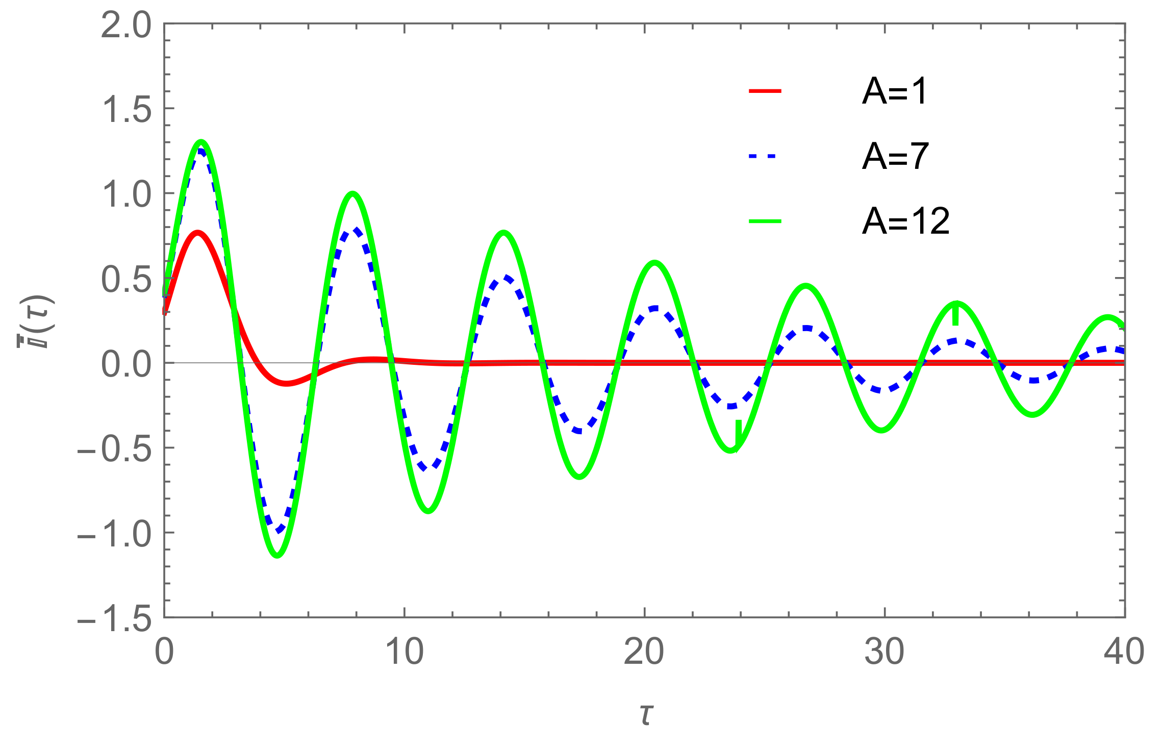
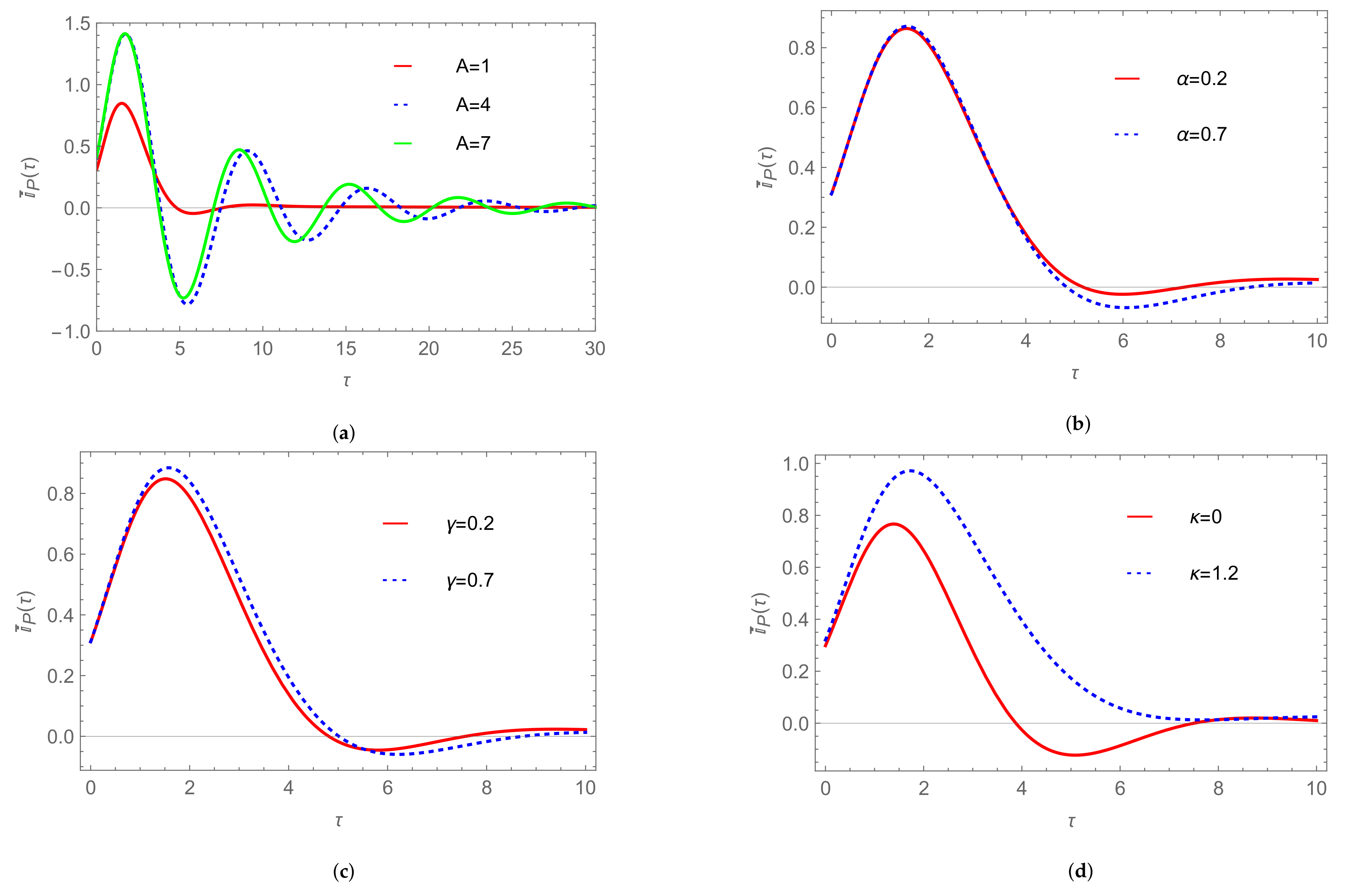
4. Fractional RLC Circuit

In the previous section, we dealt with first-order ODE and we managed to obtain the corresponding non-homogeneous contributions. Now we provide a natural further extension by studying an RLC circuit [46,47,48,49,50,51].

Problem 3 (RLC Circuit).

Regarding a second-order ODE of the type

$$\left\{\begin{array}{c}L\frac{d^2}{d{t}^2}i(t)+R\frac{d}{dt}i(t)+\frac{1}{C}i(t)=V^{\prime }(t)\hfill \\ V^{\prime }(t)=V_{0}f(t)\hfill \end{array}\right.,$$

(62)

we can proceed by just extending the outlined procedure and writing

$$\begin{array}{c}\frac{d^2}{d{\tau }^2}\overline{i}(\tau )+\frac{1}{{\omega }_0{\tau }_L}\frac{d}{d\tau }\overline{i}(\tau )+\overline{i}(\tau )=f^{*}(\tau ),\hfill \\ \overline{i}=\frac{i}{i_0},\hspace{1em}{i}_0=\frac{V_0}{L{\omega }_0^2},\hspace{1em}{\omega }_0^2=\frac{1}{LC},\hspace{1em}\tau ={\omega }_{0}t,\hspace{1em}{\tau }_L=\frac{L}{R},\hspace{1em}{f}^{*}(\tau )=\left(\frac{\tau }{{\omega }_0}\right)\hfill \end{array}$$

(63)

with L being the circuit inductance. The solution of Equation (63) for vanishing initial conditions ${\overline{i}}_0$, $\frac{d}{d\tau }\overline{i}(\tau ){\mid }_{\tau =0}$ can be written as

$$\begin{array}{cc}\hfill \overline{i}(\tau )& ={\left(\frac{d^2}{d{\tau }^2}+\frac{1}{{\omega }_0{\tau }_L}\frac{d}{d\tau }+1\right)}^{-1}{f}^{*}(\tau )={\int }_0^{\infty }{e}^{-s}\exp \left[-s\left(\frac{d^2}{d{\tau }^2}+\frac{1}{{\omega }_0{\tau }_L}\frac{d}{d\tau }\right)\right]ds f^{*}(\tau )=\hfill \\ & ={\int }_0^{\infty }{e}^{-s}\exp \left[-s\left(\frac{d^2}{d{\tau }^2}\right)\right]f^{*}\left(\tau -\frac{s}{{\omega }_0{\tau }_L}\right)ds.\hfill \end{array}$$

(64)

In order to make the previous formal solution effective, we use the identity

$$e^{-s\frac{d^2}{d{\tau }^2}}=\frac{1}{\sqrt{\pi }}{\int }_{-\infty }^{\infty }\exp \left(-{\xi }^2+2i\sqrt{s}\frac{d}{d\tau }\xi \right)d\xi$$

(65)

and eventually end up with

$$\overline{i}(\tau )=\frac{1}{\sqrt{\pi }}{\int }_0^{\infty }{e}^{-s}\left({\int }_{-\infty }^{\infty }{e}^{-{\xi }^2}{f}^{*}\left(\tau -\frac{s}{{\omega }_0{\tau }_L}+2i\sqrt{s}\xi \right)d\xi \right)ds$$

(66)

which is easily integrated and the relevant solutions are reported in Figure 12. Alternatively, when the previous solution displays convergence problems, the use of the Fourier-Transform method yields

$$\overline{i}(\tau )=\frac{1}{\sqrt{2\pi }}{\int }_{-\infty }^{\infty }\frac{{\tilde{f}}^{*}(k)e^{ik\tau }}{-k^2+\frac{ik}{{\omega }_0{\tau }_L}+1}dk .$$

(67)

Figure 12. Solution $\overline{i}(\tau )$ for different values of $A={\omega }_0{\tau }_L$.

In Figure 12 we report the current wave form for $V^{\prime }(\tau )\propto e^{-{\tau }^2}$ and different values of $A={\omega }_0{\tau }_L$. Small A values determine a strongly damped behavior.

For future convenience, we consider a capacitor defined as an operator specified in terms of fractional derivatives as

$$\hat{C}=C_0{P}^{(\alpha ,\gamma )},\hspace{1em}\hspace{1em}{P}^{(\alpha ,\gamma )}\left(\frac{d}{dt}\right)=\left(1+\frac{\kappa }{{\left(1+{\left(\tau \frac{d}{dt}\right)}^{1-\alpha }\right)}^{1-\gamma }}\right),\hspace{1em}\hspace{1em}\kappa constant.$$

(68)

whose physical meaning will be discussed in the forthcoming section and providing

$${\overline{i}}_P(\tau )=\frac{1}{\sqrt{2\pi }}{\int }_{-\infty }^{\infty }\frac{{\tilde{f}}^{*}(k)e^{ik\tau }}{-k^2+\frac{ik}{{\omega }_0{\tau }_L}+{\left(P^{(\alpha ,\gamma )}(ik)\right)}^{-1}}dk.$$

(69)

The effect of this new term on the current wave-form is provided in Figure 13.

Figure 13. Solution ${\overline{i}}_P(\tau )$ for different values of A, α, γ, κ. (a) Different values of $A={\omega }_0{\tau }_L$ with α = 0.2, γ = κ = 0.5; (b) Different values of α with A = 1, γ = κ = 0.5; (c) Different values of γ with A = 1 and α = κ = 0.5; (d) Different values of κ with A = 1 and α = γ = 0.5.

The behavior of the current, generally oscillating, exhibits a critical dependence on the various parameters defining the operator function $P^{(\alpha ,\gamma )}(.)$, whose physical meaning will be discussed in the forthcoming section.

In the previous sections we provided a solution to fractional ODE using a technique privileging the FT method. The procedure we have envisaged is useful when non-homogeneous terms are present and does not apply for homogeneous cases. We would like however to underline that the search for a solution of fractional ODE is not an easy task and a general theory is not yet available. Effective solution techniques can however be employed and, for example, the Laplace transform method offers an efficient tool, some time hampered by the difficulties encountered with the corresponding anti-transform. Before closing this section we like to quote the possibility of reducing a non-homogeneous ODE to a Volterra type integral equation [52] and apply to fractional ODE the wealth of techniques available for that problem.

5. Permittivity Models and Fractional Derivatives

5.1. Summary

Non Debye dielectrics are described by a fractional relative permittivity, which can be put in the form [25]

$${\epsilon }_r(\omega )={\epsilon }_{r_{\infty }}+\frac{{\epsilon }_{r_s}-{\epsilon }_{r_{\infty }}}{{[1+{(j\omega \tau )}^{1-\alpha }]}^{1-\beta }}$$

(70)

where ${\epsilon }_{r_{\infty }}$ and ${\epsilon }_{r_s}$ are the infinite and the static relative permittivity, $\tau$ is the principal relaxation time and $\alpha$ and $\beta$ are positive adjustable parameters between zero and one. The parameters of $\alpha$ and $\beta$ substantially determine the model used for the dielectric; it is clear that if both $\alpha$ and $\beta$ are set to zero, we obtain the standard one-pole Debye model. Apart from the Debye model, we consider other three dielectric representations whose characteristics are summarized in Table 1. In the following, for all the proposed models we assume $\tau =153$ ps.

Table 1. Dielectric models.

Model	α	β
Debye	0	0
Cole—Cole	0.4	0
Cole—Davidson	0	0.1
Havriliak—Negami	0.4	0.1

According to the formalism we have developed in the previous sections we can express the permittivity in the time-domain by replacing $\omega$ with $\frac{1}{j}\frac{d}{dt}$ thus finding

$${\epsilon }_r(\omega )\to P^{(\alpha ,\beta )}\left(\frac{d}{dt}\right)={\epsilon }_{\infty }\left(1+\frac{\kappa }{{\left(1+{\left(\tau \frac{d}{dt}\right)}^{1-\alpha }\right)}^{1-\beta }}\right),\hspace{1em}\hspace{1em}\kappa =\frac{{\epsilon }_{r,s}-{\epsilon }_{\infty }}{{\epsilon }_{\infty }}.$$

(71)

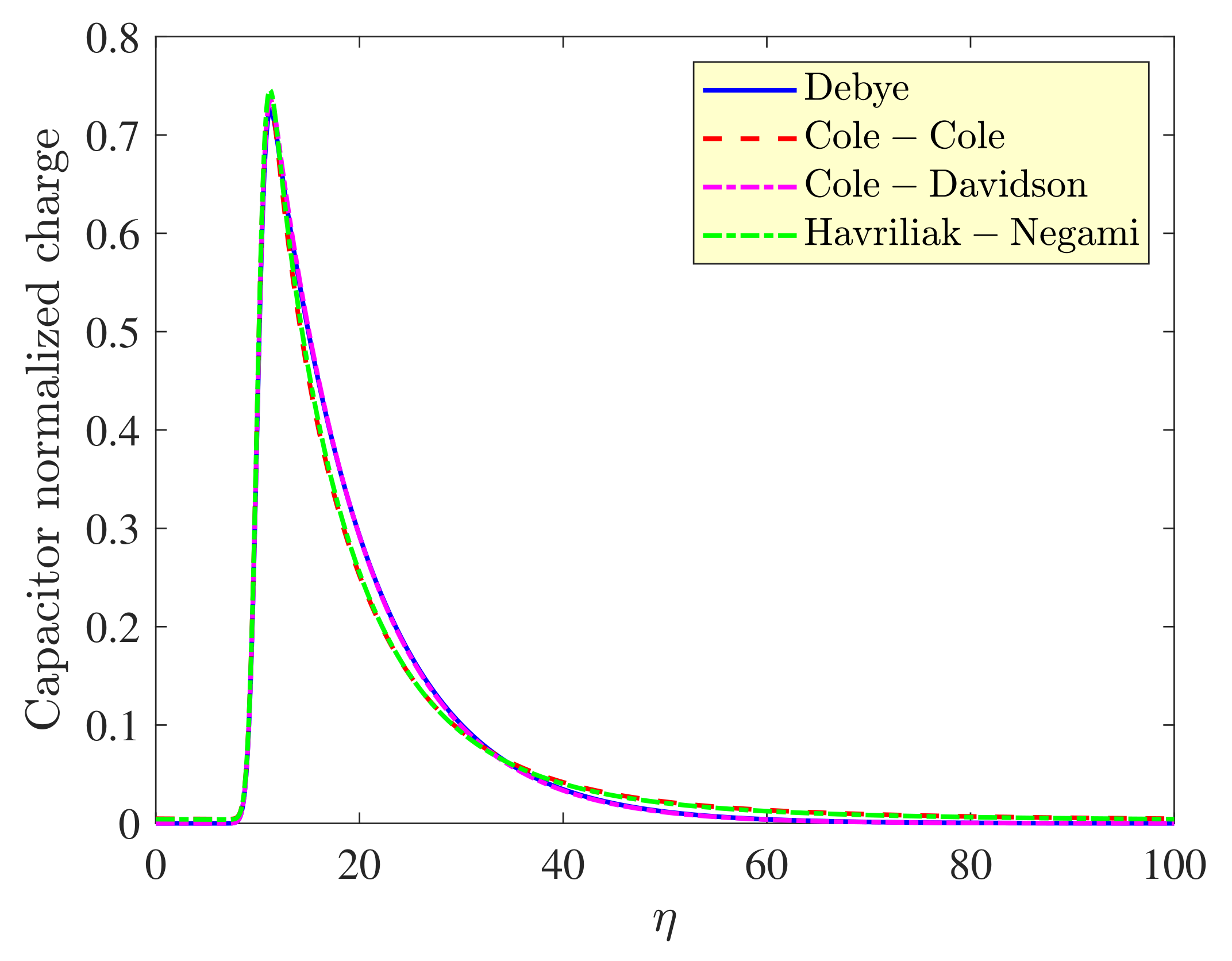
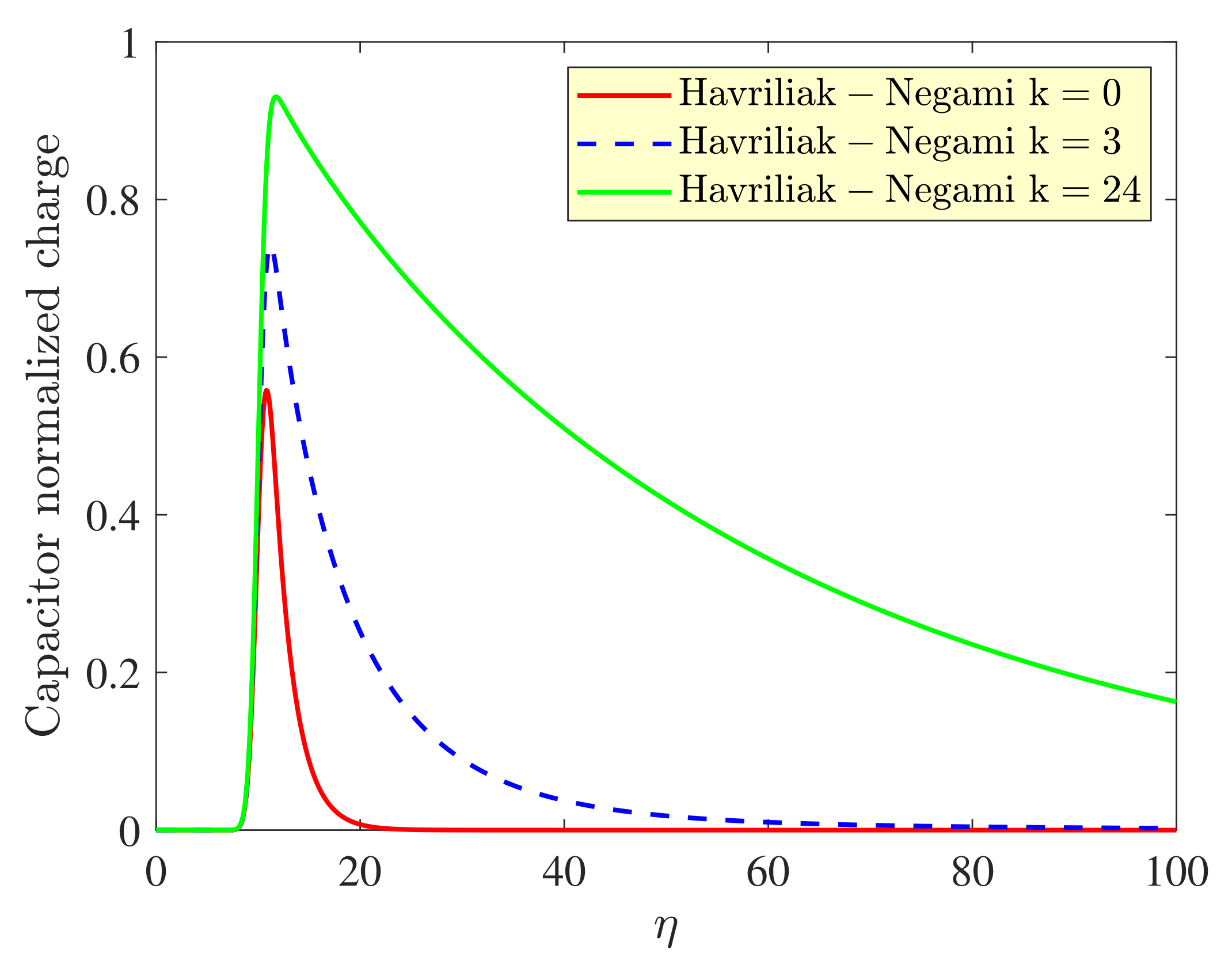
5.2. RC Circuit Tests Including Fractionary Dielectrics

The dispersive nature of dielectrics can be easily included in circuit models through the Fourier transform technique, which permits to work in the frequency domain; finally Inverse Fast Fourier Transform (IFFT) techniques can be employed to restore the time-domain behavior of the quantities under investigation. A possible very useful application for non Debye dielectric models is in the framework of the Partial Elements Equivalent Circuit (PEEC) method, an integral equation based method that permits performance of electromagnetic (EM) simulations of complex structures introducing a circuit representation of the EM phenomena. The PEEC method is very useful in Electromagnetic Compatibility (EMC) and Signal integrity (SI) areas, allowing prediction and solving of electromagnetic interference (EMI) issues.

Dielectric materials are a fundamental part of modern electric and electronic devices and for this reason it is important to accurately include their presence; this can be done in the PEEC method through the concept of excess capacitance [53]. In PEEC models is feasible to include in the excess capacitance also the fractional relative permittivity of Equation (70), in order to provide a more accurate representation of the EM phenomena that affect the structures under observation.

It is reported here the example of an RC series circuit fed by a Gaussian pulse voltage, with the capacitor supposed to consist of flat and parallel plates, filled by a dielectric characterized by a relative permittivity generally described by Equation (70); all the four dielectric laws presented are examined here.

The ordinary differential equation, describing an RC series circuit through the electric charge $q(t)$ in the time-domain, is the following:

$$R\frac{d}{dt}q(t)+\frac{q(t)}{C(t)}=V(t)=V_{0}f(t),$$

(72)

where R is the resistance value of the RC circuit and $V(t)=V_{0}f(t)$ is the forcing function which represents the voltage source applied to the circuit; the capacitance $C(t)$ is a time-dependent function because of the dispersive nature of the dielectric inside the capacitor. In the frequency domain, the capacitor can be described by its complex capacitance

$$C(\omega )={\epsilon }_0{\epsilon }_r(\omega )\frac{S}{d}=C_0{\epsilon }_r(\omega ),$$

(73)

where S is the surface of the plates and d is the distance between them. Therefore, its time-domain counterpart is of the form

$$C(t)=C_0{\epsilon }_r(t)$$

(74)

where

$${\epsilon }_r(t)={\epsilon }_{\infty }\left(1+\frac{\kappa }{{(1+{(\tau \frac{d}{dt})}^{(1-\alpha )})}^{(1-\beta )}}\right)$$

(75)

is the time-domain fractional dielectric law described in Equation (71).

We now define the parameter: ${\tau }_c=R{C}_0$ and introduce the dimensionless variable $\eta =\frac{t}{{\tau }_c}$. Hence, the forcing function $f(t)$ is also a $f({\tau }_c\eta )=f^{*}(\eta )$ and the variable function $q(t)$ is also expressible as a $q({\tau }_c\eta )$. The last positions permit the writing of Equation (72) as

$$R\frac{d}{dt}q({\tau }_c\eta )+\frac{q({\tau }_c\eta )}{C(t)}=V_0{f}^{*}(\eta ).$$

(76)

By considering that $dt={\tau }_{c}d\eta$ and the Equation (74), we write Equation (76) as

$$\frac{R}{{\tau }_c}\frac{d}{d\eta }q({\tau }_c\eta )+\frac{q({\tau }_c\eta )}{C_0{\epsilon }_r(t)}=V_0{f}^{*}(\eta )$$

(77)

which, using the relation ${\tau }_c=R{C}_0$ and expressing that ${\epsilon }_r(t)={\epsilon }_r({\tau }_c\eta )$, becomes

$$\frac{1}{C_0}\frac{d}{d\eta }q({\tau }_c\eta )+\frac{q({\tau }_c\eta )}{C_0{\epsilon }_r({\tau }_c\eta )}=V_0{f}^{*}(\eta ).$$

(78)

By introducing the parameter $q_0=C_0{V}_0$, which has the dimensions of the electric charge, we can write

$$\frac{d}{d\eta }q({\tau }_c\eta )+\frac{q({\tau }_c\eta )}{{\epsilon }_r({\tau }_c\eta )}=q_0{f}^{*}(\eta )$$

(79)

and finally we can obtain the differential equation for the normalized charge $\tilde{q}({\tau }_c\eta )$ in the normalized variable $\eta$

$$\frac{d}{d\eta }\tilde{q}({\tau }_c\eta )+\frac{\tilde{q}({\tau }_c\eta )}{{\epsilon }_r({\tau }_c\eta )}=f^{*}(\eta ),$$

(80)

where the relative permittivity can be expressed as

$${\epsilon }_r({\tau }_c\eta )={\epsilon }_{\infty }\left(1+\frac{\kappa }{{(1+{(\frac{\tau }{{\tau }_c}\frac{d}{d\eta })}^{(1-\alpha )})}^{(1-\beta )}}\right).$$

(81)

A solution of the Equation (80) can be found first by expressing it in the frequency domain, where $\frac{d}{d\eta }=jk$, k being the dimensionless pulsation

$$jk\tilde{Q}(k)+\frac{\tilde{Q}(k)}{{\epsilon }_r(k)}=F^{*}(k),$$

(82)

where $\tilde{Q}(k)$ is the Fourier transform with respect to the variable $\eta$ of the normalized charge $\tilde{q}({\tau }_c\eta )$. Furthermore, it is necessary to express the fractional dielectric permittivity law in the dimensionless frequency domain as

$${\epsilon }_r(k)={\epsilon }_{\infty }\left(1+\frac{\kappa }{{(1+{(\frac{\tau }{{\tau }_c}jk)}^{(1-\alpha )})}^{(1-\beta )}}\right).$$

(83)

Finally, in the frequency domain, we have the following final expression for the normalized charge

$$\tilde{Q}(k)=\frac{F^{*}(k)}{\frac{1}{{\epsilon }_r(k)}+jk}$$

(84)

where $F^{*}(k)$ is the Fourier transform of $f^{*}(\eta )$.

We considered a forcing function $f^{*}(\eta )=e^{-{(\eta -10)}^2}$, represented in Figure 14, and the data for the test in Table 2.

Figure 14. Normalized source voltage.

Table 2. Data for the test.

τ	153 ps
${\tau }_c$	$88.54$ ps
$\kappa$	3
${\epsilon }_{\infty }$	2

The function ${\tilde{q}}^{*}(\eta )$ is restored by the IFFT algorithm, which is an approximation of the integral below.

$${\tilde{q}}^{*}(\eta )=\frac{1}{2\pi }{\int }_{-\infty }^{+\infty }\frac{F^{*}(k)}{{\left[{\epsilon }_{\infty }\left(1+\frac{\kappa }{{(1+{(\frac{\tau }{{\tau }_c}jk)}^{(1-\alpha )})}^{(1-\beta )}}\right)\right]}^{-1}+jk}{e}^{jk\eta }dk$$

(85)

The results for the time-domain behavior of the normalized charge using the IFFT technique are depicted in Figure 15. It is clear, from Figure 15, that considering different frequency domain dielectric laws for the capacitor changes necessarily also the time-domain behavior of the overall circuit.

Figure 15. Time-domain behavior of the normalized charge using the four dielectric laws proposed.

In order to validate the IFFT technique, in Figure 16 is reported a comparison with the approximated integral computation, for the Havriliak–Negami model, showing a very good agreement between the two techniques. Moreover, it is possible to observe in Figure 17 the normalized charge behavior for a dielectric described by the Havriliak–Negami model, considering three different values of the parameter $\kappa$.

Figure 16. Time-domain comparison for the normalized charge considering the Havriliak–Negami dielectric.

Figure 17. Solution with $\tau =153$, $\alpha =0.4$, $\beta =0.1$ and different values of $\kappa$.

The main advantage of the IFFT technique is its simplicity and ease of coding. On the other hand, its inclusion in a 3D time-stepping electromagnetic solver is not straightforward since it requires an a priori knowledge of the source term in the integral (Figure 15) which is not the case when the fractionary dielectric is part of a more complex 3D model. In this case, recursive schemes are recommended which are based on the knowledge of a rational approximation of the fractional permittivity.

6. Final Comments

This article has been devoted to the use of mathematical tools, employing operational calculus, for the solution of non-homogeneous fractional ODEs. We have noted that fractional calculus is an extension of ordinary calculus, having the merit of dealing with a new point of view to the differential calculus, expressed in terms of integral operators, interpreted as non-integer derivatives. Even though not explicitly stated, the distinguishing feature of such a formalism is the use of operators suited to deal with non-local problems and physical mechanisms employing memory effects as e.g., dissipation in various materials [3].

We started our discussion considering the search for a solution of the Lamb–Bateman equation, a genuine non-local problem, by the use of a purely operational technique and we have shown that, by keeping the freedom of treating differential operators as ordinary algebraic quantities, we have been able to provide a “natural” meaning for the derivatives of fractional order. In order to corroborate the point we have just raised, we discuss an example from Ref. [54] and mention that the Abel integral equation of the first kind is given by

$$f(x)={\int }_0^x\frac{k(x,s)g(s)}{{(x-s)}^{\alpha }}ds,\hspace{1em}\hspace{1em}0<\alpha <1,\hspace{1em}0\le x\le b,$$

(86)

where $g(s)$ is the unknown, b is an upper limit specified by the nature of the kernel $k(x,s){(x-s)}^{-\alpha }$. By assuming that it is just a constant (the unit in our example) we easily obtain the solution, which is contained in the definition of Caputo derivative given in Equation (12); we find indeed

$$\frac{1}{\Gamma (1-\alpha )}f(x)= {\partial }_x^{\alpha -1}g(x)$$

(87)

which, once inverted yields

$$g(x)=\frac{1}{\Gamma (1-\alpha )}{\partial }_x^{1-\alpha }f(x)=\frac{1}{\Gamma (1-\alpha )\Gamma (\alpha )}{\int }_0^x\frac{f^{\prime }(\xi )}{{(x-\xi )}^{1-\alpha }}d\xi .$$

(88)

The example is underscored to stress the interplay between the concept of fractional derivatives and integral operators.

Regarding the second point we have raised (non-locality), we would like to mention the spinless relativistic Schrodinger’s equation [9], which, in terms of pseudo-operators, reads

$$\left\{\begin{array}{c}i {\partial }_{\tau }\mathsf{\Psi }(\eta ,\tau )=\sqrt{(1-{\partial }_{\eta }^2)}\mathsf{\Psi }(\eta ,\tau )\hfill \\ \mathsf{\Psi }(\eta ,0)=\psi (\eta )\hfill \end{array}\right.,$$

(89)

where the operator on the left realizes a pseudo fractional operator. According to what we have learned so far we can cast Equation (89) in the form [13,55]

$$\left\{\begin{array}{c}i {\partial }_{\tau }\mathsf{\Psi }(\eta ,\tau )=(1-{\partial }_{\eta }^2)\mathsf{\Phi }(\eta ,\tau )\hfill \\ \mathsf{\Phi }(\eta ,\tau )={(1-{\partial }_{\eta }^2)}^{-\frac{1}{2}}\mathsf{\Psi }(\eta ,\tau )=\frac{1}{\Gamma \left(\frac{1}{2}\right)}{\int }_0^{\infty }{e}^{-s}\frac{e^{s{\partial }_{\eta }^2}}{\sqrt{s}}\mathsf{\Psi }(\eta ,\tau )ds\hfill \end{array}\right..$$

(90)

The exponential operator containing the second-order derivative is a diffusion operator, whose action on a given function is provided by the so-called Gauss–Weierstrass transform, namely

$$e^{\alpha {\partial }_x^2}f(x)=\frac{1}{2\sqrt{\pi \alpha }}{\int }_{-\infty }^{\infty }{e}^{-\frac{{(\sigma -x)}^2}{4\alpha }}f(\sigma )d\sigma$$

(91)

which holds if the integral on the r.h.s. converges. Therefore, in conclusion, we find

$$\mathsf{\Phi }(\eta ,\tau )=\frac{1}{2\pi }{\int }_0^{\infty }\frac{e^{-s}}{s}\left({\int }_{-\infty }^{\infty }{e}^{-\frac{{(\sigma -\eta )}^2}{4s}}\mathsf{\Psi }(\sigma ,\tau )d\sigma \right)ds.$$

(92)

We accordingly transformed the original problem containing the square root of a differential operator into an integro-differential equation in which the non-locality is specified by a kind of diffusive kernel. The relevant solution is not easy to achieve using this form, which is however amenable for a perturbative expansion. We furthermore employed a solution procedure based on an evolution operator and Fourier transform method to solve Equation (89). By using a Gaussian as the initial function, we obtain the result reported in Figure 18, where we showed the square modulus of the wave function $\mathsf{\Psi }(\eta ,\tau )$ at different times. The relevant evolution is characterized by an asymmetric diffusion, including a shift of the peak and the development of a long tail. We also checked that this behavior is compatible (at short times) with the results obtained with the perturbative solution.

Figure 18. $\mid \mathsf{\Psi }(\eta ,\tau ){\mid }^2$ vs. $\eta$ for different values of $\tau$, by reference to Equation (89).

The use of pseudo-operators, involving square roots of derivative operators in relativistic Quantum Mechanics is delicate either from the mathematical and physical points of view. However, it is scientifically sound and does not imply any doubtful steps. The operators on both sides of Equation (89) are indeed hermitian, and the associated evolution operator is unitary. This is the minimum requirement when a Quantum Mechanics problem is posed, since the physical consequences from the associated mathematical treatment is not flawed by intrinsic “fatal” errors.

Some authors “generalize” the Schroedinger equation by directly replacing (time or spatial) derivative with fractional counterparts. The development of a credible formulation of Fractional Quantum Mechanics (FQM), requires the change of the specific paradigms leading to the formulation of the Schroedinger equation itself. For this reason, in Ref. [56], the problem has been afforded starting from a path integral formulation. This study has led to the conclusion that standard Quantum Mechanics follows from the fractality of Brownian motion and FQM deepen its root into the fractality of Lévy flights. The formal basis of the (non-relativistic) FQM has been considered with adequate mathematical rigor. The Schroedinger equation derived in [56] reads

$$\left\{\begin{array}{c}i\hslash {\partial }_t \psi ={\hat{H}}_a \psi \hfill \\ {\hat{H}}_a=-D_a{(\hslash {\partial }_x)}^a+V(x)\hfill \end{array}\right.$$

(93)

where $D_a$ is a constant, adjusting the associated physical units and defining the link between energy and momentum in FQM [56]. The operator on the r.h.s. of Equation (93) is not Hermitian; this implies that the associated eigenvalues are not real and the corresponding evolution operator is not unitary. An important possibility within this respect is offered by the formalism adopted in dissipative Quantum Mechanics [57] whose mathematical (and physical as well) treatment requires the use of bi-orthogonal states [56,57] yielding a more appropriate definition of the operator self-adjointedness condition and a correct tool for the evaluation of matrix elements between different quantum states.

Regarding the Free Particle evolution, Equation (93) yields

$$\psi (\xi ,\sigma )=e^{i T_{\alpha } \sigma {({\partial }_{\xi })}^{\alpha }}{\psi }_0(\xi ),\hspace{1em}\hspace{1em}\xi =\frac{x}{{\mathrm{ƛ}}_c},\hspace{1em}{\mathrm{ƛ}}_c=\frac{\hslash }{mc},\hspace{1em}\sigma ={\displaystyle \frac{ct}{{\mathrm{ƛ}}_c}},\hspace{1em}{T}_{\alpha }=\frac{D_{\alpha }}{c}{\hslash }^{\alpha -1}$$

(94)

where we used a more convenient non-dimensional form. The solution of Equation (94) can be obtained using the discussed method. Using the definition of the Riesz fractional derivative [56,58], we obtain the behavior reported in Figure 19. It is qualitatively similar to that displayed in Figure 18, thus suggesting a non-local nature of the underlying dynamics.

Figure 19. $\mid \psi (\xi ,\sigma ){\mid }^2$ vs. $\xi$ for different $\sigma$ values.

In order to complete this discussion, we would like to add as a further example of application of the discussion so far developed to the solution of propagation equations of D’Alembert type, namely

$$\left\{\begin{array}{c}{\overrightarrow{\nabla }}^{2}U-\frac{1}{v^2}{\partial }_t^{2}U=0,\hspace{1em}\hspace{1em}U(x,y,z,0)=f(x,y,z),\hfill \\ {\partial }_{t}U(x,y,z,t){\mid }_{t=0}=g(x,y,z),\hspace{1em}\hspace{1em}{\overrightarrow{\nabla }}^2={\partial }_x^2+{\partial }_y^2+{\partial }_z^2.\hfill \end{array}\right.$$

(95)

The use of the generalization of the evolution operator method [59] allows casting of the solution of Equation (95) in the form

$$\begin{array}{cc}\hfill U(x,y,z,t)& =\frac{1}{2}{e}^{vt\sqrt{{\partial }_x^2+{\partial }_y^2+{\partial }_z^2}}\left[f(x,y,z)+{\left(\sqrt{{\partial }_x^2+{\partial }_y^2+{\partial }_z^2}\right)}^{-1}g(x,y,z)\right]+\hfill \\ & +\frac{1}{2}{e}^{-vt\sqrt{{\partial }_x^2+{\partial }_y^2+{\partial }_z^2}}\left[f(x,y,z)-{\left(\sqrt{{\partial }_x^2+{\partial }_y^2+{\partial }_z^2}\right)}^{-1}g{(x,y,z)}^{-1}\right].\hfill \end{array}$$

(96)

which can be handled by the use of standard numerical means, including Fourier transform techniques.

The same procedure can be applied to the paraxial approximation of (96) and to the treatment of problems involving e.g., diffraction or Quantum Mechanics problems. In this case more sophisticated and advanced methods, developed in Refs. [60,61,62,63] can be exploited as discussed in a forthcoming paper.

This is only a part of the discussion, we have underscored that the meaning of the fractional electric circuit is a vague concept if not merged within a proper context. We have also mentioned that the Ohm law itself should be reformulated to better justify the use of non-integer derivatives. As already noted in Ref. [64], these reasons are simple and physically motivated. There are no physical phenomena with an infinite speed of change and the correct description should take into account relaxation processes. If the relaxation process is rapid and the relaxation time is negligible with respect to the entire observation time at issue, no memory effect arises and no necessity for fractional calculus emerges. On the other side, when the processes at issue are with timescales comparable to the relaxation times, the histories (the memories) should be taken into account that lead to the use of the memory formalism (history integrals) and the fractional calculus approach.

Within this context, we note that the Ohm law should be replaced by the integral form

$$I(t)=\frac{1}{R}{\int }_0^t{(t-z)}^{-\mu }U(z)dz,\hspace{1em}\hspace{1em}0<\mu <1,$$

(97)

which is easily restated in terms of a Caputo derivative. This point opens further issues on the role of the power laws ruling the relaxation times processes [64]. We have just mentioned these topics which deserve a more appropriate analysis, which is to be presented elsewhere.

References

1. Oldham, K.B.; Spanier, J. The Fractional Calculus: Theory and Applications of Differentiation and Integration to Arbitrary Order; Mathematics in Science and Engineering; Elsevier: Amsterdam, The Netherlands, 1974; Volume 111. [Google Scholar]
2. Kilbas, A.A.; Srivastava, H.M.; Trujillo, J.J. Theory and Applications of Fractional Differential Equations; Elsevier: Amsterdam, The Netherlands, 2006. [Google Scholar]
3. Uchaikin, V. Fractional Derivatives for Physicists and Engineers; Springer: Berlin, Germany, 2013. [Google Scholar]
4. Samko, S.G.; Kilbas, A.A.; Marichev, O.I. Fractional Integrals and Derivatives, Theory and Applications; Gordon and Breach Science Publishers: Langhorne, PA, USA, 1993. [Google Scholar]
5. Podlubny, I. Fractional Differential Equations; Academic Press: New York, NY, USA, 1999. [Google Scholar]
6. Baleanu, D.; Diethelm, K.; Scalas, E.; Trujillo, J.J. Fractional Calculus Models and Numerical Methods; World Scientific Publishing Company: New York, NY, USA, 2012. [Google Scholar]
7. Dattoli, G.; Torre, A.; Quattromini, M. Miscellaneous results on the theory of evolution operators and generalized transformations. Il Nuovo Cim.-Soc. B 1999, 6, 693–708. [Google Scholar]
8. Heaviside, O. Electromagnetic Induction and Its Propagation; The Electrician: 1887. Available online: https://www.gsjournal.net/Science-Journals/Historical%20Papers-Mechanics%20/%20Electrodynamics/Download/6897 (accessed on 13 August 2021).
9. Bjorken, J.D.; Drell, S. Relativistic Quantum Mechanics; McGraw-Hill: New York, NY, USA, 1965. [Google Scholar] [CrossRef] [Green Version]
10. Baym, G. Lectures on Quantum Mechanics; Taylor & Francis Group: Boca Raton, FL, USA; CRC Press: Boca Raton, FL, USA, 1969; ISBN 9780805306675. [Google Scholar]
11. Babusci, D.; Dattoli, G.; Quattromini, M. Relativistic equations with fractional and pseudodifferential operators. Phys. Rev. A 2011, 83, 062109. [Google Scholar] [CrossRef] [Green Version]
12. Babusci, D.; Dattoli, G.; Quattromini, M.; Sabia, E. Relativistic harmonic oscillator, the associated equations of motion, and algebraic integration methods. Phys. Rev. E 2013, 87, 033202. [Google Scholar] [CrossRef]
13. Dattoli, G.; Sabia, E.; Gorska, K.; Horzela, A. Relativistic wave equations: An operational approach. J. Phys. A Math. Theor. 2015, 48, 125203. [Google Scholar] [CrossRef] [Green Version]
14. Barkai, E. Fractional Fokker-Planck equation, solution, and application. Phys. Rev. E 2001, 63, 046118. [Google Scholar] [CrossRef] [PubMed] [Green Version]
15. Yen, C.S.; Fazarinc, Z.; Wheeler, R.L. Time-domain skin-effect model for transient analysis of lossy transmission lines. Proc. IEEE 1982, 70, 750–757. [Google Scholar]
16. Cho, S.; Kim, K.R.; Park, B.-G.; Kang, I.M. Non-quasi-static modeling of silicon nanowire metal-oxide-semiconductor field-effect transistor and its model verification up to 1 THz. Jpn. J. Appl. Phys. 2010, 49, 110206. [Google Scholar] [CrossRef]
17. Shang, Y.; Fei, W.; Yu, H. Fractional-order transmission line modeling. Int. J. Adv. Comput. Sci. Technol. 2013, 2, 18–24. [Google Scholar]
18. Shang, Y.; Yu, H.; Fei, W. Design and Analysis of CMOS-Based Terahertz Integrated Circuits by Causal Fractional-Order RLGC Transmission Line Model. IEEE J. Emerg. Sel. Top. Circuits Syst. 2013, 3, 355–366. [Google Scholar] [CrossRef]
19. Al-Daloo, M.; Soltan, A.; Yakovlev, A. Advance Interconnect Circuit Modeling Design Using Fractional-Order Elements. IEEE Trans. Comput. Aided Des. Integr. Circuits Syst. 2020, 39, 2722–2734. [Google Scholar] [CrossRef]
20. Esser, A.T.; Smith, K.C.; Gowrishankar, T.R.; Weaver, J.C. Towards solid tumor treatment by nanosecond pulsed electric fields. Technol. Cancer Res. Treat. 2009, 8, 289–306. [Google Scholar] [CrossRef] [Green Version]
21. Rekanos, I.T. FDTD Schemes for Wave Propagation in Davidson-Cole Dispersive Media Using Auxiliary Differential Equations. IEEE Trans. Antennas Propag. 2012, 60, 1467–1478. [Google Scholar] [CrossRef]
22. Rekanos, I.T. FDTD Modeling of Havriliak-Negami Media. IEEE Microw. Wirel. Compon. Lett. 2012, 22, 49–51. [Google Scholar] [CrossRef]
23. Tofighi, M. FDTD Modeling of Biological Tissues Cole–Cole Dispersion for 0.5–30 GHz Using Relaxation Time Distribution Samples—Novel and Improved Implementations. IEEE Trans. Microw. Theory Tech. 2009, 57, 2588–2596. [Google Scholar] [CrossRef]
24. Abdullah, H.H.; Elsadek, H.A.; ElDeeb, H.E.; Bagherzadeh, N. Fractional Derivatives Based Scheme for FDTD Modeling of nth-Order Cole–Cole Dispersive Media. IEEE Antennas Wirel. Propag. Lett. 2012, 11, 281–284. [Google Scholar] [CrossRef]
25. Mescia, L.; Bia, P.; Caratelli, D. Fractional Derivative Based FDTD Modeling of Transient Wave Propagation in Havriliak–Negami Media. IEEE Trans. Microw. Theory Tech. 2014, 62, 1920–1929. [Google Scholar] [CrossRef]
26. Lamb, H. On the diffraction of a solitary wave. Proc. Lond. Math. Soc. 1910, 28, 422–437. [Google Scholar] [CrossRef] [Green Version]
27. Martin, P.A. Harry Bateman: From Manchester to Manuscript Project. Available online: https://studylib.net/doc/13384560/harry-bateman-from-manchester-to-manuscript-project (accessed on 13 August 2021).
28. Babusci, D.; Dattoli, G.; Sacchetti, D. The Lamb-Bateman integral equation and the fractional derivatives. Fract. Calc. Appl. Anal. 2011, 14, 317–320. [Google Scholar] [CrossRef] [Green Version]
29. Babusci, D.; Dattoli, G.; Licciardi, S.; Sabia, E. Mathematical Methods for Physics; World Scientific: Singapore, 2019. [Google Scholar]
30. Caputo, M. Linear models of dissipation whose Q is almost frequency independent. Geophys. J. R. Astr. Soc. 1967, 13, 529–539. [Google Scholar] [CrossRef]
31. Caputo, M. Elasticitá e Dissipazione; Zanichelli: Bologna, Italy, 1969. [Google Scholar]
32. Caputo, M.; Fabrizio, M. Applications of new time and spatial fractional derivatives with exponential kernels. Progr. Fract. Differ. Appl. 2016, 2, 1–11. [Google Scholar] [CrossRef]
33. Gorenflo, R.; Mainardi, F. Fractional calculus. Integral and differential equations of fractional order. In Fractals and Fractional Calculus in Continuum Mechanics; Carpinteri, A., Mainardi, F., Eds.; Springer: Wien, NY, USA, 1997; pp. 223–276. [Google Scholar]
34. Licciardi, S. Umbral Calculus, a Different Mathematical Language. Ph.D. Thesis, Department of Mathematics and Computer Sciences, XXIX Cycle, University of Catania, Catania, Italy, 2018. [Google Scholar]
35. Dattoli, G.; Górska, K.; Horzela, A.; Penson, K.A.; Sabia, E. Theory of relativistic heat polynomials and one-sided Lévy distributions. J. Math. Phys. 2017, 58, 063510. [Google Scholar] [CrossRef] [Green Version]
36. Górska, K.; Horzela, A. The higher-order heat-type equations via signed Lévy stable and generalized Airy functions. J. Phys. A Math. Theor. 2013, 46, 425001. [Google Scholar] [CrossRef] [Green Version]
37. Dattoli, G.; Ottaviani, P.L.; Torre, A.; Vazquez, L. Evolution operator equations: Integration with algebraic and finite difference methods. Applications to physical problems in classical and quantum mechanics and quantum field theory. Riv. Nuovo Cim. 1997, 20, 3. [Google Scholar] [CrossRef]
38. Anderssen, R.S.; Husain, S.A.; Loy, R.J. The Kohlrausch function: Properties and applications. Anziam J. 2004, 45, C800–C816. [Google Scholar] [CrossRef] [Green Version]
39. Górska, K.; Horzela, A. Lévy stable distributions via associated integral transform. J. Math. Phys. 2012, 53, 053302. [Google Scholar] [CrossRef] [Green Version]
40. Penson, K.A.; Górska, K. Exact and Explicit Probability Densities for One-Sided Lévy Stable Distributions. Phys. Rev. Lett. 2010, 105, 210604. [Google Scholar] [CrossRef] [PubMed] [Green Version]
41. Feynman, R. The Feynman Lectures on Physics; California Institute of Technology, Michael A. Gottlieb and Rudolf Pfeiffer: Pasadena, CA, USA, 1964; Volume II, Chapter 22. [Google Scholar]
42. Mittag-Leffler, M.G. Une généralisation de l’intégrale de Laplace-Abel. Comptes Rendus Hebd. Séances l’Académie Sci. 1903, 136, 537–539. [Google Scholar]
43. Weisstein, E.W. Mittag-Leffler Function, from MathWorld—A Wolfram Web Resource. Available online: http://mathworld.wolfram.com/Mittag-LefflerFunction.html (accessed on 13 August 2021).
44. Dattoli, G.; Gorska, K.; Horzela, A.; Licciardi, S.; Pidatella, R.M. Comments on the Properties of Mittag-Leffler Function. Eur. Phys. J. Spec. Top. 2017, 226, 3427–3443. [Google Scholar] [CrossRef] [Green Version]
45. Gorenflo, R.; Loutschko, J.; Luchko, Y. Computation of the Mittag–Leffler function and its derivatives. Fract. Calc. Appl. Anal. 2002, 5, 491–518. [Google Scholar]
46. Gomez, F.; Rosales, J.; Guia, M. RLC electrical circuit of non-integer order. Cent. Eur. J. Phys. 2013, 11, 1361–1365. [Google Scholar] [CrossRef] [Green Version]
47. Guia, M.; Gomez, F.; Rosales, J. Analysis of the time and frequency domain for the RC electric circuit of fractional order. Cent. Eur. J. Phys. 2013, 11, 1366–1371. [Google Scholar]
48. Atangana, A.; Nieto, J.J. Numerical solution for the model of RLC circuit via the fractional derivative without singular kernel. Adv. Mech. Eng. 2015, 7. [Google Scholar] [CrossRef]
49. Atangana, A.; Badr, S.T.A. Extension of the RLC electrical circuit to fractional derivative without singular kernel. Adv. Mech. Eng. 2015, 7, 1–6. [Google Scholar]
50. Alsaedi, A.; Nieto, J.J.; Vencatesh, V. Fractional electric circuits. Mech. Eng. Adv. 2015. [Google Scholar] [CrossRef]
51. Shah, P.V.; Patel, A.D.; Salehbhai, I.A.; Shukla, A.K. Analytic solution for the RLC electric circuit model in fractional order. Abstr. Appl. Anal. 2014, 24, 343814. [Google Scholar]
52. Artioli, M.; Dattoli, G.; Licciardi, S.; Pagnutti, S. Fractional Derivatives, Memory kernels and solution of Free Electron Laser Volterra type equation. Mathematics 2017, 5, 73. [Google Scholar] [CrossRef] [Green Version]
53. Ruehli, A.; Antonini, G.; Jiang, L. PEEC Models for Dielectrics. In Circuit Oriented Electromagnetic Modeling Using the PEEC Techniques; John Wiley & Sons: New York, NY, USA, 2017; pp. 249–283. [Google Scholar] [CrossRef]
54. Jahanshahi, S.; Babolian, E.; Torres, D.F.M.; Vahidi, A. Solving Abel integral equations of first kind via fractional calculus. J. King Saud Univ. Sci. 2015, 27, 161–167. [Google Scholar] [CrossRef] [Green Version]
55. Dattoli, G.; Giannessi, L.; Quattromini, M.; Torre, A. Exponential operators, operational rules and evolution problems. Il Nuovo C. B 1998, 113, 699. [Google Scholar]
56. Laskin, N. Fractional Schroedinger equation. Phys. Rev. E 2002, 66, 056108. [Google Scholar] [CrossRef] [PubMed] [Green Version]
57. Dattoli, G.; Torre, A.; Mignani, R. Non Hermitian Evolution of Two-Level Quantum Systems. Phys. Rev. A 1990, 42, 1467. [Google Scholar] [CrossRef]
58. Hermann, R. Fractional Calculus: An Introduction for Physicists; World Scientific: Hackensack, NJ, USA, 2011; ISBN 978-981-4340-24-3. [Google Scholar]
59. Dattoli, G.; Ricci, P.E.; Khomasuridze, I. Operational methods, special polynomial and functions and solution of partial differential equations. Int. Transf. Spec. Funct. 2004, 15, 309–321. [Google Scholar] [CrossRef]
60. Baskakov, V.A.; Popov, A.V. Implementation of transparent boundaries for numerical solution of the Schroedinger equation. Wave Motion 1991, 14, 123–128. [Google Scholar] [CrossRef]
61. Popov, A.V. Accurate modeling of transparent boundaries in quasi-optics. Radio Sci. 1996, 31, 1781–1790. [Google Scholar] [CrossRef]
62. Antoine, X.; Arnold, A.; Besse, C.; Ehrhardt, M.; Schadle, A. A review of transparent and artificial boundary conditions techniques for linear and nonlinear Schroedinger equations. Commun. Comput. Phys. 2008, 4, 729–796. [Google Scholar]
63. Feshchenko, R.M.; Popov, A.V. Exact transparent boundary condition for the three-dimensional Schroedinger equation in a rectangular cuboid computational domain. Phys. Rev. E 2013, 88, 053308. [Google Scholar] [CrossRef]
64. Hristov, J. Electrical Circuits of Non-integer Order: Introduction to an Emerging Interdisciplinary Area with Examples. In Analysis and Simulation of Electrical and Computer Systems; Mazur, D., Golębiowski, M., Korkosz, M., Eds.; Lecture Notes in Electrical Engineering; Springer: Cham, Switzerland, 2017; Volume 452. [Google Scholar] [CrossRef]