Dual-Input Slope Seeking Control of Continuous Micro-Algae Cultures with Experimental Validation

Featured Application

The production of algal biomass or of a product associated with biomass growth can be optimized by manipulating the dilution rate and the incident light intensity in indoor photo-bioreactors. However, model-based optimization is delicate in view of the time and experimental efforts required to develop sufficiently accurate dynamic models. Extremum seeking provides an alternative real-time optimization approach, where prior model knowledge is not required, and only a measurable (or estimable) performance index is needed online.

Abstract

This paper investigates the application of adaptive slope-seeking strategies to dual-input single output dynamic processes. While the classical objective of extremum seeking control is to drive a process performance index to its optimum, this paper also considers slope seeking, which allows driving the performance index to a desired level (which is thus sub-optimal). Moreover, the consideration of more than one input signal allows minimizing the input energy thanks to the degrees of freedom offered by the additional inputs. The actual process is assumed to be locally approachable by a Hammerstein model, combining a nonlinear static map with a linear dynamic model. The proposed strategy is based on the interplay of three components: (i) a recursive estimation algorithm providing the model parameters and the performance index gradient, (ii) a slope generator using the static map parameter estimates to convert the performance index setpoint into slope setpoints, and (iii) an adaptive controller driving the process to the desired setpoint. The performance of the slope strategy is assessed in simulation in an application example related to lipid productivity optimization in continuous cultures of micro-algae by acting on both the incident light intensity and the dilution rate. It is also validated in experimental studies where biomass production in a continuous photo-bioreactor is targeted.

1. Introduction

Extremum Seeking Control (ESC) is a Real-Time Optimization (RTO) technique used to drive a measurable process performance index to its optimum following direct input adaptation [1]. In the classical scheme proposed in [2], a sinusoidal dither signal ensures the persistency of excitation of the input and filters are used to extract the gradient information from output measurements. This gradient is forced to zero on average so as to converge to a close neighborhood of the optimal operating point. An interesting feature of ESC is that limited a priori knowledge about the process under consideration is required in order to perform RTO. Although this approach has become popular following the stability proof provided in [3] and the intrinsic simplicity of the scheme [4,5,6], it suffers from the three time-scale separation (implying slow convergence) and its heuristic tuning procedure.

Various approaches have been proposed to improve the convergence rate. In [7], a proportional integral scheme is introduced to improve the transient behavior while [8] uses a recursive least square (RLS) algorithm to estimate online the parameters of a linear model approximating the process input/output static map. However, in [9], the authors point out that the latter approach generally leads to a biased estimation of the optimal operating point when dealing with dynamic systems. It is therefore necessary to account for those dynamics, and in order to preserve simplicity and avoid the need for extensive prior knowledge about the process, a black-box approach is preferable, for instance using Wiener–Hammerstein models [10,11].

Extension of ESC to multiple-inputs–single-output (MISO) process optimization has also provided interesting results both in simulation and experiments. In [12], the classical scheme is extended to achieve maximum power tracking of PV panels with an experimental validation. In [13], an extended Kalman filter is used to estimate the gradient and Hessian of a static quadratic dual-input–single-output (DISO) map to remove thermo-acoustic instabilities in an atmospheric combustor test rig. In applications such as PV panels or wind turbine power generation, it is sometimes required to operate at a given sub-optimal operating point so as to adjust the production to the actual load/demand. In this regard, slope seeking control (SSC) [14] provides the possibility of optimal and suboptimal setpoint tracking. In [15,16], the authors propose an adaptive SSC for a class of SISO dynamic processes, and a numerical validation is provided with biomass productivity optimization in microalgae cultures.

In this work, an extension of adaptive slope seeking a DISO dynamic processes is proposed. To this end, the process under consideration is assumed to be approachable at least locally with a quadratic block-oriented model in the form of a Hammerstein model. Adaptive slope seeking allows driving the process either at the extremum of the measurable performance index or an intermediate operating point specified via the slope of the performance index. The degrees of freedom offered by the additional input can be used in various ways, for instance, to minimize the input energy. A recursive extended least squares (RELS) algorithm is used to estimate online the model parameters. To alleviate the tedious and generally heuristic integrator gain tuning procedure of the classical filter-based ES/SOP control, a pole placement controller (PPC) is used, which was introduced by the authors in [15,16].

The performance of the slope seeking strategy is first assessed in a simulation example related to lipid productivity optimization in continuous cultures of micro-algae by acting on both the incident light intensity and the dilution rate. During the last decade, microalgae cultures have indeed received some attention from the real-time optimization research community (see for instance [17,18,19,20,21]).

The proposed strategy is then further validated in a lab-scale experimental study of the cultures of the micro-algae Scenedesmus obliquus in a flat-panel photo-bioreactor (PBR).

The paper is organized as follows: Section 2 introduces the main assumptions regarding the dynamic process under consideration and describes the dual-input adaptive slope seeking strategy. In Section 3, the estimation algorithm used to infer the static map and dynamic model parameters is presented. Section 4 is devoted to slope reference generation and proposes two algorithms offering the possibility to minimize one or both inputs. Section 5 presents a pole placement controller applied to drive the process to the selected set-point. In Section 6, the performance of the slope-seeking strategy is assessed with a simulation example related to the optimization of the lipid production in continuous cultures of micro-algae in photobioreactors, while an experimental validation is proposed in Section 7. Finally, some conclusions and perspectives are drawn.

2. A DISO Adaptive Slope-Seeking Strategy

The control strategy is built upon the assumption that the process can be described by a block-oriented model, which is made of the interconnection of nonlinear static building blocks and linear time-invariant dynamic building blocks. A great variety of configurations are possible, including series and parallel structures. In this study, we restrict ourselves to the classical Hammerstein model, where a nonlinear static block followed by a linear dynamical model represent process and sensor dynamics. Such block-oriented models are often used to model nonlinear systems [22], and in the following, we will consider a class of systems that can be modeled locally using quadratic static building blocks and second-order linear time invariant dynamic blocks:

Assumption 1.

The process input/output static map can be approximated locally by a quadratic function of the form:

$$x\left(k\right)={\underline{u}}^{T}A\underline{u}+{\underline{b}}^T\underline{u}+c$$

(1)

where $\underline{u}$ represents the input vector and x the output of the nonlinear static block, $A\in {\mathbb{R}}^{m\times m}$, $b\in {\mathbb{R}}^{m\times 1}$, $c\in \mathbb{R}$ and $\underline{u}\in {\mathbb{R}}^{m\times 1}$, with m being the number of inputs.

This first assumption implies that (i) driving the system to a stable steady-state manifold is feasible and that (ii) the system in the steady state is likely to be a convex/concave function of the input. In bioprocess applications, these statements find their justifications in the bifurcation analysis developed in [23], which can be considered as a basis for further investigations of bioprocesses [24].

Assumption 2.

The actuator, process and sensor dynamics can be approximated locally by linear time-invariant dynamic blocks. In particular, they can be described by proper and stable second-order transfer functions with unitary steady-state gains:

$$G\left(z^{-1}\right)=K\frac{1+{\gamma }_1{z}^{-1}+{\gamma }_2{z}^{-2}}{1+{\beta }_1{z}^{-1}+{\beta }_2{z}^{-2}}$$

(2)

with $K=\frac{1+{\beta }_1+{\beta }_2}{1+{\gamma }_1+{\gamma }_2}$ and $z^{-1}$ the back-shift operator such that $z^{-1}x\left(k\right)=x(k-1)$.

The relatively slow dynamics of (bio)processes allows considering the latter in steady state and to consequently isolate the fast actuator dynamics in a separate block. The low-order approximation of the process nonlinearity and dynamics is justified by the fact that an adaptive control approach will be developed, where the parameters of the block-oriented models are estimated online. The estimation of these parameters requires persistency of excitation of the input signals, which corresponds to the following assumption:

Assumption 3.

Input signals are persistently exciting and allow closed-loop parameter estimation of the block-oriented models.

In practice, this is achieved using appropriate dither signals in the gradient estimation algorithm, such as pseudo-random binary sequences [25,26]. This point will be further elaborated in the subsequent sections.

Using the notation of Assumptions 1 and 2, the quadratic DISO Hammerstein model can be described by the following state-space model:

$$\begin{array}{cc}\hfill x\left(k\right)=& {\underline{u}}^{T}A\underline{u}+b^T\underline{u}+c\hfill \\ \hfill J\left(k\right)=& -{\beta }_{1}J(k-1)-{\beta }_{2}J(k-2)\hfill \end{array}$$

(3a)

$$\begin{array}{cc}\hfill & +Kx\left(k\right)+K{\gamma }_{1}x(k-1)+K{\gamma }_{2}x(k-2)\hfill \end{array}$$

(3b)

where J is the measured performance index.

A last assumption is now required regarding the existence of a unique extremum (maximum) point of the measurable performance index:

Assumption 4.

The performance index is concave, or in other words, there exists a unique set of inputs ${\underline{u}}^{opt}\in {\mathbb{R}}^{m\times 1}$ such that:

$$\begin{array}{cc}\hfill & \nabla J=\left[\begin{array}{c}\frac{\partial J}{\partial u_1}\\ \frac{\partial J}{\partial u_2}\end{array}\right]=0\hfill \end{array}$$

(4a)

$$\begin{array}{cc}\hfill & {\nabla }^{2}J=A\prec 0\hfill \end{array}$$

(4b)

ensuring that there exists a stabilizing input vector ${\underline{u}}^{opt}$ driving the process performance index to its maximum $J^{max}$.

As discussed in [27], this restriction can be relaxed in the multi-modal case provided an adequate dither signal design.

In the adaptive SSC depicted in Figure 1, a RELS algorithm is used to estimate online the static map matrices $[A,b,c]$, which feed a slope reference generator [15] whose role is to convert a desired reference $J_{ref}$ into a corresponding gradient reference $\nabla J{|}_{ref}$.

This allows driving the process to the optimal performance index (where $\nabla J=0$) or to an intermediate, sub-optimal index (where $\nabla J\ne 0$). The regulation is effected by comparing the gradient estimate $\widehat{\nabla J}$ provided by the recursive estimator to the slope reference. The set-point deviation $\widehat{ϵ}=\widehat{\nabla J}-\nabla J{|}_{ref}$ has to be driven to zero by a controller such that:

$$\begin{array}{c}\hfill ϵ=0⟹\nabla J=\nabla J{|}_{ref}⟹J=J_{ref}\end{array}$$

(5)

Note that the optimal value of the performance index does not need to be known a priori. The controller will achieve optimal performance by enforcing $\nabla J{|}_{ref}=0$. When a suboptimal operating point is selected, a non-zero reference is specified for the slope of the performance index. It is in principle possible to operate the plant to the left of the optimum (positive slope) or to the right (negative slope), depending on the process dynamics and stability behavior. As none of these values are a priori known, this procedure will require some form of trial and error by the process operator. It should also be noticed that (5) is only valid if Assumption A4 is locally verified, i.e., in a concave neighborhood. However, information about the achievable optimum and the sensitivity in the vicinity of the optimum is quickly collected in the course of the first experiment. In addition, when a suboptimal operation point is selected, the energy of one or both input signals can be reduced. This is interesting from an economical point of view if the considered process consumes expensive resources. This latter point will be elaborated in the future.

A detailed stability analysis of this scheme is outside the scope of this paper, but stability should be guaranteed under Assumptions 1–4. More details on stability analysis of discrete-time ESC can be found in [2,28], and some results for multivariable ESC can be found in [29,30].

3. The Recursive Estimation Algorithm

This section develops a Recursive Extended Least Squares (RELS) estimator of the parameters of the quadratic Hammertein model.

3.1. Basic Concepts

Consider the output-error auto-regressive (OEAR) system [31]:

$$y\left(k\right)=y_s\left(k\right)+\eta \left(k\right)$$

(6)

where $y_s={\psi }_s^T{\theta }_s$ is the noise-free output of the process (in the previous developments, it represents the noise-free performance index J) and

$$\eta \left(k\right)=\frac{1}{C\left(z^{-1}\right)}\nu \left(k\right)$$

(7)

is the output of an Auto-Regressive (AR) process with $\nu$, a white noise with zero mean and variance ${\sigma }^2$, and $C\left(z^{-1}\right)=1+c_1{z}^{-1}+c_2{z}^{-2}+\cdots +c_{n_c}{z}^{-n_c}$ is a stable polynomial of order $n_c$.

Equation (6) can be rewritten as:

$$y={\psi }^T\theta ={\left[\begin{array}{cc}{\psi }_s& {\psi }_n\end{array}\right]}^T\left[\begin{array}{c}{\theta }_s\\ {\theta }_n\end{array}\right]={\psi }_s^T{\theta }_s+{\psi }_n^T{\theta }_n$$

(8)

where $w\left(k\right)={\psi }_n^T{\theta }_n$ is the noise regression model, where

$$\begin{array}{cc}\hfill {\psi }_n^T& =\left[\begin{array}{cccc}\eta (k-1)& \eta (k-2)& \cdots & \eta (k-n_c)\end{array}\right]\hfill \end{array}$$

(9a)

$$\begin{array}{cc}\hfill {\theta }_n& ={\left[\begin{array}{cccc}{c}_1& c_2& \cdots & c_{n_c}\end{array}\right]}^T\hfill \end{array}$$

(9b)

In the following, it is assumed that $n_c=2$.

Given structure (8), the unknown parameters $\theta$ can be estimated online using a RELS algorithm [31] in the form:

$$\begin{array}{cc}\hfill e\left(k\right)& =y_{meas}\left(k\right)-\psi {(k-1)}^T\widehat{\theta }(k-1)\hfill \end{array}$$

(10a)

$$\begin{array}{cc}\hfill P\left(k\right)& =\frac{1}{\lambda }\left[\begin{array}{c}P(k-1)-\frac{P(k-1)\psi (k-1)\psi {(k-1)}^{T}P(k-1)}{\lambda +\psi {(k-1)}^{T}P(k-1)\psi (k-1)}\end{array}\right]\hfill \end{array}$$

(10b)

$$\begin{array}{cc}\hfill \widehat{\theta }\left(k\right)& =\widehat{\theta }(k-1)+P\left(k\right)\psi (k-1)e\left(k\right)\hfill \end{array}$$

(10c)

where $e\left(k\right)$ is the a priori estimation error, $y_{meas}\left(k\right)$ the measured output, and $P\left(k\right)$ the covariance matrix of the parameter estimation error $\theta -\widehat{\theta }\left(k\right)$ at sample k. As a result, the RELS computes online estimates of both the noise-free and noise model regression parameters contained, respectively, in ${\theta }_s$ and ${\theta }_n$. The forgetting factor $\lambda$ determines how fast past data are disregarded, and typically $0.85\le \lambda \le 0.99$. An estimation of $\eta \left(k\right)$ is provided by the a posteriori estimation error $ϵ\left(k\right)=y_{meas}\left(k\right)-\psi {(k-1)}^T\widehat{\theta }\left(k\right)$.

The RELS algorithm is generally coupled with a constant trace algorithm, ensuring a sufficient correction gain to track slowly time varying parameters. A regularization of the covariance matrix $P\left(k\right)$ is obtained as:

$$\overline{P}\left(k\right)=\frac{k_{0}P\left(k\right)}{Trace\left(P\right(k\left)\right)}$$

(11)

In addition, a projection algorithm [32] can be added to enforce estimator stability by introducing prior knowledge about some parameter bounds:

$$\widehat{\theta }=\left\{\begin{array}{ccc}\widehat{\theta }\hfill & ,if\hfill & \widehat{\theta }\in \mathcal{D}\hfill \\ {\widehat{\theta }}_{Proj}\hfill & ,if\hfill & \widehat{\theta }\notin \mathcal{D}\hfill \end{array}\right.$$

(12)

where:

$${\widehat{\theta }}_{Proj}=\left\{\begin{array}{ccc}\widehat{\theta }-\frac{P(:,i)}{P(i,i)}\left[\begin{array}{c}\widehat{{\theta }_i}-{\widehat{{\theta }_i}}^{+}\end{array}\right]\hfill & ,if\hfill & \widehat{{\theta }_i}>{\widehat{{\theta }_i}}^{+}\hfill \\ \widehat{\theta }+\frac{P(:,i)}{P(i,i)}\left[\begin{array}{c}{\widehat{{\theta }_i}}^{-}-\widehat{{\theta }_i}\end{array}\right]\hfill & ,if\hfill & \widehat{{\theta }_i}<{\widehat{{\theta }_i}}^{-}\hfill \end{array}\right.$$

(13)

The domain $\mathcal{D}$ is defined for $i\in 1,\cdots ,n_{\theta }$, $n_{\theta }$ being the number of parameters such that:

$$\mathcal{D}:=\{\widehat{\theta }\in \mathcal{D},{\widehat{{\theta }_i}}^{-}\le \widehat{{\theta }_i}\le {\widehat{{\theta }_i}}^{+}\}$$

(14)

3.2. Application to the Quadratic Hammerstein Model

Using the quadratic Hammerstein model introduced in (3) with $m=2$ and without coupling terms (we consider $a_{12}=0$ to simplify the developments and because we observed that these terms have little impact on the performance of the controllers), $A=\left[\begin{array}{cc}{a}_{11}& 0\\ 0& a_{22}\end{array}\right]\in {\mathbb{R}}^{2\times 2}$, $\underline{b}=\left[\begin{array}{c}{b}_1\\ b_2\end{array}\right]\in {\mathbb{R}}^{2\times 1}$, $c\in \mathbb{R}$ and $\underline{u}=\left[\begin{array}{c}{u}_1\\ u_2\end{array}\right]\in {\mathbb{R}}^{2\times 1}$, the development of (3a) gives:

$$x\left(k\right)=a_{11}{u}_1^2\left(k\right)+b_1{u}_1\left(k\right)+a_{22}{u}_2^2\left(k\right)+b_2{u}_2\left(k\right)+c$$

(15)

This expression can be inserted into (3b), which yields:

$$\begin{array}{cc}\hfill J\left(k\right)=& -{\beta }_{1}J(k-1)-{\beta }_{2}J(k-2)+K[a_{11}{u}_1^2\left(k\right)+b_1{u}_1\left(k\right)+a_{22}{u}_2^2\left(k\right)\hfill \\ \hfill & +b_2{u}_2\left(k\right)+c]\hfill \\ \hfill & +K{\gamma }_1[a_{11}{u}_1^2(k-1)+b_1{u}_1(k-1)+a_{22}{u}_2^2(k-1)\hfill \\ \hfill & +b_2{u}_2(k-1)+c]\hfill \\ \hfill & +K{\gamma }_2[a_{11}{u}_1^2(k-2)+b_1{u}_1(k-2)+a_{22}{u}_2^2(k-2)\hfill \\ \hfill & +b_2{u}_2(k-2)+c]\hfill \end{array}$$

(16)

This equation can be cast in the form of a product between a regressor of informative signals ${\psi }_s$ and the parameter vector ${\theta }_s$:

$$\begin{array}{cc}\hfill J\left(k\right)=& {\psi }_s^T(k-1){\theta }_s\hfill \\ \hfill {\psi }_s^T(k-1)=& \{-J(k-1),-J(k-2),\hfill \\ \hfill & u_1^2\left(k\right),u_1\left(k\right),u_2^2\left(k\right),u_2\left(k\right),\hfill \\ \hfill & u_1^2(k-1),u_1(k-1),u_2^2(k-1),u_2(k-1),\hfill \\ \hfill & u_1^2(k-2),u_1(k-2),u_2^2(k-2),u_2(k-2),\hfill \end{array}$$

(17a)

$$\begin{array}{cc}\hfill & 1\}\hfill \\ \hfill {\theta }_s=& \{{\beta }_1,{\beta }_2,K{a}_{11},K{b}_1,K{a}_{22},K{b}_2,\hfill \\ \hfill & K{\gamma }_1{a}_{11},K{\gamma }_1{b}_1,K{\gamma }_1{a}_{22},K{\gamma }_1{b}_2,\hfill \\ \hfill & K{\gamma }_2{a}_{11},K{\gamma }_2{b}_1,K{\gamma }_2{a}_{22},K{\gamma }_2{b}_2,\hfill \end{array}$$

(17b)

$$\begin{array}{cc}\hfill & (1+{\beta }_1+{\beta }_2){c\}}^T\hfill \end{array}$$

(17c)

The model parameters can be extracted from the vector ${\theta }_s$ in (17c) as:

$$\begin{array}{cc}\hfill & {\widehat{\beta }}_1={\widehat{\theta }}_{s1}\hfill \end{array}$$

(18a)

$$\begin{array}{cc}\hfill & {\widehat{\beta }}_2={\widehat{\theta }}_{s2}\hfill \end{array}$$

(18b)

$$\begin{array}{cc}\hfill & {\widehat{\gamma }}_1=\frac{{\widehat{\theta }}_{s7}}{{\theta }_{s3}}\hfill \end{array}$$

(18c)

$$\begin{array}{cc}\hfill & {\widehat{\gamma }}_2=\frac{{\widehat{\theta }}_{s11}}{{\theta }_{s3}}\hfill \end{array}$$

(18d)

$$\begin{array}{cc}\hfill & {\widehat{a}}_{11}=\frac{{\widehat{\theta }}_{s3}+{\widehat{\theta }}_{s7}+{\widehat{\theta }}_{s11}}{1+{\widehat{\theta }}_{s1}+{\widehat{\theta }}_{s2}}\hfill \end{array}$$

(18e)

$$\begin{array}{cc}\hfill & {\widehat{b}}_1=\frac{{\widehat{\theta }}_{s4}+{\widehat{\theta }}_{s8}+{\widehat{\theta }}_{s12}}{1+{\widehat{\theta }}_{s1}+{\widehat{\theta }}_{s2}}\hfill \end{array}$$

(18f)

$$\begin{array}{cc}\hfill & {\widehat{a}}_{22}=\frac{{\widehat{\theta }}_{s5}+{\widehat{\theta }}_{s9}+{\widehat{\theta }}_{s13}}{1+{\widehat{\theta }}_{s1}+{\widehat{\theta }}_{s2}}\hfill \end{array}$$

(18g)

$$\begin{array}{cc}\hfill & {\widehat{b}}_2=\frac{{\widehat{\theta }}_{s6}+{\widehat{\theta }}_{s10}+{\widehat{\theta }}_{s14}}{1+{\widehat{\theta }}_{s1}+{\widehat{\theta }}_{s2}}\hfill \end{array}$$

(18h)

$$\begin{array}{cc}\hfill & \widehat{c}=\frac{{\widehat{\theta }}_{s15}}{(1+{\widehat{\theta }}_{s1}+{\widehat{\theta }}_{s2})}\hfill \end{array}$$

(18i)

The second-order transfer function representing the system dynamics can be considered with either two, one, or no zeros (which implies, respectively, that ${\gamma }_1\ne 0$ and ${\gamma }_2\ne 0$, or ${\gamma }_1\ne 0$ and ${\gamma }_2=0$, or ${\gamma }_1={\gamma }_2=0$). Let us denote $R{M}_{n_p{m}_z}$ the regression model with $n_p$ poles and $m_z$ zeros.

Table 1. Model configurations and corresponding simplifications.

Regression Model	Equation	Parameters Equal to 0 or Signals to be Omitted	Parameter Subscript Changes	Δ Length of ${\mathit{\theta }}_{\mathit{s}}$
$R{M}_{2p1z}$	(18)	${\theta }_{s11},{\theta }_{s12},{\theta }_{s13},{\theta }_{s14}$ $u_i^2(k-1),u_i(k-1),i\in \{1,2\}$	${\theta }_{s15}\to {\theta }_{s11}$	$15\to 11$
$R{M}_{2p0z}$	(18)	${\theta }_{s7},{\theta }_{s8},{\theta }_{s9},{\theta }_{s10},{\theta }_{s11},{\theta }_{s12},{\theta }_{s13},{\theta }_{s14}$ $u_i^2(k-j),u_i(k-j),i,j\in \{1,2\}$	${\theta }_{s15}\to {\theta }_{s7}$	$15\to 7$

lists some possible simplifications.

3.3. Persistency of Excitation

To avoid practical parameter identifiability issues using the RLS algorithm, it is recommended to use an input signal with a sufficiently rich frequency bandwidth as discussed in [25,26]. While using a pseudo-random binary signal (PRBS) with limited amplitude and sufficient signal to noise ratio is generally advised for linear systems, amplitude-modulated pseudo-random binary signals and multi-levels pseudo-random signals (MPRS) have been shown to be more appropriate for nonlinear system identification [33,34].

A PRBS is a periodic and deterministic signal with white-noise-like properties [35]. This signal is generated by adding a sequence of shift register specific outputs in a $XOR$ gate in closed-loop. The sequence length is computed as $L=2^N-1$, where N is the number of shift registers in the sequence. The sequence duration is obtained as $L{T}_{prbs}$ with $T_{prbs}=p{T}_s$, the PRBS sampling period expressed as a multiple $p\in {\mathbb{N}}^{+}$ of the process sampling time $T_s$. Further details about PRBS generation can be found in [31,35].

In this work, it is proposed to generate MPRS by adding three PRBS with different bandwith (sampling time) and shift register sequences inducing a longer period and both amplitude and holding time modulations. Furthermore, this approach allows maximal amplitude and minimal holding time specifications. For DISO processes identification, using such design procedure may also help reducing spectral overlap between inputs when required.

4. Slope Reference Generator

As introduced in Section 2, the purpose of the slope reference generator (see Figure 1) is to convert the desired performance index set-point $J_{ref}\le J^{max}$ into corresponding gradient references $\nabla J{|}_{re{f}_{\left(k\right)}}=\left[\begin{array}{c}\frac{\partial J}{\partial u_1}\\ \frac{\partial J}{\partial u_2}\end{array}\right]{|}_{re{f}_k}$.

Consider the quadratic static map, where the dependency on time k is omitted to simplify the notation, and more importantly, the actuator/sensor dynamics is neglected (as we are interested in generating the slope reference signals).

$$\begin{array}{cc}\hfill J=& a_{11}{u}_1^2+b_1{u}_1+a_{22}{u}_2^2+b_2{u}_2+c\hfill \\ \hfill =& a_{22}{u}_2^2+b_2{u}_2+c^{\prime }\left(u_1\right)\hfill \end{array}$$

(19)

where

$$\begin{array}{cc}\hfill c^{\prime }\left(u_1\right)=& a_{11}{u}_1^2+b_1{u}_1+c\hfill \end{array}$$

(20)

The cost function gradient is given by:

$$\nabla J=\left[\begin{array}{c}2a_{11}{u}_1+b_1\\ 2a_{22}{u}_2+b_2\end{array}\right]$$

(21)

A set $U_2\left(u_1\right)$ of control inputs $u_2$ driving the process performance index J to a desired value $J_{ref}$ can be computed as the set of solutions of the second order polynomial Equation (19):

$$U_2\left(u_1\right)=\frac{-b_2\pm \sqrt{|b_2^2-4a_{22}(c^{\prime }\left(u_1\right)-J_{ref})}|}{2a_{22}}$$

(22)

From an operational and economical point of view, it can be interesting to drive the process output to a desired set-point while minimizing one of the inputs or both.

Considering the positiveness of $u_2$, the gradient of $U_2$ with respect to $u_1$ reads:

$$\frac{\partial U_2}{\partial u_1}=\frac{-b_1-2a_{11}{u}_1}{\sqrt{|b_2^2-4a_{22}(a_{11}{u}_1^2+b_1{u}_1-J_{ref}+c)|}}$$

(23)

The value of $u_1$ minimizing $u_2$ such that $J=J_{ref}$ is computed by setting

$$\frac{\partial U_2}{\partial u_1}=0$$

(24)

which yields:

$$u_1^s=-\frac{b_1}{2a_{11}}$$

(25)

and the corresponding minimal value of $u_2$ is computed by replacing $u_1$ by $u_1^s$ in (22). It should be noticed that the positiveness of the inputs $u_1$ and $u_2$, combined with (25) and the concavity of J ($a_{11}$ and $a_{22}$ are strictly negative parameters), imposes that $b_1$ and $b_2$ are positive. Therefore, the derivative (23) is negative when $u_1<u_1^s$ and positive when $u_1>u_1^s$, and (22) presents a minimum in $u_1^s$.

These results are compiled in Algorithm 1, which summarizes the design procedure for slope reference generation either for extremum seeking (ESC) or suboptimal setpoint (SOP) with minimization/maximization of one input ($u_2$).

Algorithm 1 Adaptive slope reference generation algorithm for DISO processes ESC and SOP with minimization/maximization of one input

1: procedure$\nabla J{|}_{re{f}_{\left(k\right)}}$($\widehat{A},\widehat{b},\widehat{c}$, Objective, $J_{re{f}_{\left(k\right)}}$, Model) 2:     if Objective == ’ESC’ then 3:          $$\nabla J{|}_{re{f}_{\left(k\right)}}=\left[\begin{array}{c}0\\ 0\end{array}\right]$$ 4:     else                ▹ Objective == ’SOP with $u_2$ optimization’ 5:         Select a desired Performance index set-point: $J_{re{f}_{\left(k\right)}}$. 6:         Compute $u_{1_k}^s$, the value of $u_1$ minimizing (maximizing) $u_{2_k}$ such that $J=J_{re{f}_{\left(k\right)}}$ given parameter estimates at iteration k: $$u_{1_k}^s=-\frac{{\widehat{b}}_1}{2{\widehat{a}}_{11}}$$ 7:         and substitute in (20) and (22) to obtain: $$\begin{array}{cc}\hfill u_{2_k}^{min}\left(J_{re{f}_{\left(k\right)}}\right)=& \frac{-{\widehat{b}}_2-\sqrt{|{\widehat{b}}_2^{\prime 2}-4{\widehat{a}}_{22}({\widehat{c}}^{\prime }\left(u_{1_{k-1}}^s\right)-J_{re{f}_{\left(k\right)}})}|}{2{\widehat{a}}_{22}},{\widehat{a}}_{22}\ne 0\hfill \\ \hfill u_{2_k}^{max}\left(J_{re{f}_{\left(k\right)}}\right)=& \frac{-{\widehat{b}}_2+\sqrt{|{\widehat{b}}_2^{\prime 2}-4{\widehat{a}}_{22}({\widehat{c}}^{\prime }\left(u_{1_{k-1}}^s\right)-J_{re{f}_{\left(k\right)}})}|}{2{\widehat{a}}_{22}},{\widehat{a}}_{22}\ne 0\hfill \end{array}$$ 8:         Deduce the gradient reference: $$\nabla J{|}_{re{f}_{\left(k\right)}}=\left[\begin{array}{c}2{\widehat{a}}_{11}{u}_{1_k}^s+{\widehat{b}}_1\\ 2{\widehat{a}}_{22}{u}_{2_k}^{min}+{\widehat{b}}_2\end{array}\right]$$ 9:     endif 10:    return $\nabla J{|}_{re{f}_{\left(k\right)}}$

Algorithm 2 considers a suboptimal setpoint tracking with minimization of both inputs. Starting from arbitrary initial conditions $u_{1_0}$ and $u_{2_0}$, the algorithm iterates to estimate the minimal values $u_{1_k}^{min}$ and $u_{2_k}^{min}$ based on the previous estimates $u_{2_{k-1}}^{min}$ and $u_{1_{k-1}}^{min}$ and the static map parameter estimates at time k.

Algorithm 2 Adaptive slope reference generation algorithm for DISO processes—SOP with minimization of both inputs

1: procedure$\nabla J{|}_{re{f}_{\left(k\right)}}$($\widehat{A},\widehat{b},\widehat{c}$, $J_{re{f}_{\left(k\right)}}$, Model) 2:     Select a desired Performance index set-point: $J_{re{f}_{\left(k\right)}}$. 3:     Compute $u_{1_k}^{min}$ and $u_{2_k}^{min}$, respectively, based on $u_{2_{k-1}}^{min}$ and $u_{1_{k-1}}^{min}$ as: $$\begin{array}{cc}\hfill u_{i_k}^{min}\left(J_{re{f}_{\left(k\right)}}\right)=& \frac{-{\widehat{b}}_i^{\prime }-\sqrt{|{\widehat{b}}_i^2-4{\widehat{a}}_{ii}({\widehat{c}}^{\prime }\left(u_{j_{k-1}}^{min}\right)-J_{re{f}_{\left(k\right)}})}|}{2{\widehat{a}}_{ii}},{\widehat{a}}_{ii}\ne 0\hfill \end{array}$$ $i,j\in \{1,2\}$ with $i\ne j$. 4:     Deduce the gradient reference: $$\nabla J{|}_{re{f}_{\left(k\right)}}=\left[\begin{array}{c}2{\widehat{a}}_{11}{u}_{1_k}^{min}+{\widehat{b}}_1\\ 2{\widehat{a}}_{22}{u}_{2_k}^{min}+{\widehat{b}}_2\end{array}\right]$$ 5:     return $\nabla J{|}_{re{f}_{\left(k\right)}}$

5. Controller Design

The model under consideration requires two parallel SISO controllers: one for the regulation of the input/output pair $u_1/\frac{\partial J}{\partial u_1}$ and another for $u_2/\frac{\partial J}{\partial u_2}$. To this end and to replace the classical ESC integral controller of Figure 1, a pole placement controller (PPC) introduced by the authors in [15,16] is investigated.

At time k, the gradient of the performance index with respect to the input signal $u_i$, $i\in \{1,2\}$ is given by:

$${\left(\begin{array}{c}\frac{\partial J}{\partial u_i}\end{array}\right)}_{k+1}=2a_{ii}\left(k\right)u_i(k-1)+b_i\left(k\right)$$

(26)

This expression can be cast into the form of a state-space model

$$\begin{array}{ccc}\hfill x_{k+1}& =& A_d{x}_k+B_d{u}_k+w_k\hfill \\ \hfill y_k& =& C_d{x}_k\hfill \end{array}$$

(27)

with the following correspondence: $x_k={\left(\begin{array}{c}\frac{\partial J}{\partial u_i}\end{array}\right)}_k$, $A_d=0$, $B_d=2a_{ii}$, $C_d=1$. $b_i\left(k\right)$ is considered as a perturbation $w_k=b_i\left(k\right)$.

To ensure zero steady-state error under step disturbances, an integral action is introduced and pole-placement allows imposing a first-order closed-loop dynamic behavior. The dominant pole imposes the settling time $t_s$ and the non-dominant pole is selected to be much faster, so as to allow for a fast transient. Using the certainty equivalence principle [31,36], $a_{ii}$ is replaced by its estimate ${\widehat{a}}_{ii}$ and the controller gain is updated at each innovation.

Although the control algorithm depends on the estimation provided by the recursive algorithm, the $PPC$ design is based on only one parameter $a_{ii}$, which allows one to maintain some robustness level. Further, placing the closed-loop poles allows taking the a priori neglected dynamics into account. There is indeed a three time-scale defined by the estimator (the fastest), the linear dynamics, and the controller (the slowest), which should be respected during the pole placement procedure. The following simulation study will highlight these elements.

6. A Simulation Study: Optimization of Micro-Algae Lipid Productivity

Microalgae growth in a bioreactor can be described by the Droop model [37], which assumes that extracellular nutrient S is stored in a so-called internal quota Q, before being used for biomass X growth. The Droop Model is usually the cornerstone of more elaborated models accounting for light-related phenomena [38].

For the model under consideration, nutrient uptake $\rho$ is described by a Michaelis–Menten type kinetics with internal quota limitation:

$$\rho (S,Q)={\rho }_{max}\frac{S}{S+K_S}(1-\frac{Q}{Q_{max}})$$

(28)

whereas the growth rate is modelled by Droop kinetics and photo-inhibition is incorporated through Haldane kinetics:

$$\mu (Q,I)={\mu }_{max}\left(1-\frac{Q_{min}}{Q}\right)\frac{I}{I+K_{sI}I+\frac{I^2}{K_{iI}}}$$

(29)

In these expressions, $K_S$ is the half-saturation constant with respect to substrate S, $Q_{min}$ is the quota threshold below which no growth is possible, and $Q_{max}$ is the maximum nitrogen quota. ${\rho }_{max}$, ${\mu }_{max}$, $K_{sI}$ and $K_{iI}$ are, respectively, the maximum uptake and growth rates, the half-saturation and the inhibition constants with respect to incident light intensity.

To keep the model simple, photo-acclimation is described by a first-order dynamics:

$$\left\{\begin{array}{ccc}\hfill & {\tau }_I\frac{d\overline{I}}{dt}& =I-\overline{I}\hfill \\ \hfill & \mu (Q,\overline{I})& ={\mu }_{max}\left(1-\frac{Q_{min}}{Q}\right)\frac{\overline{I}}{\overline{I}+K_{sI}\overline{I}+\frac{{\overline{I}}^2}{K_{iI}}}\hfill \end{array}\right.$$

(30)

Mass balances in the chemostat lead to the following set of ordinary differential equations:

$$\begin{array}{cc}\hfill \frac{dX}{dt}& =\mu (Q,I)X-DX\hfill \end{array}$$

(31a)

$$\begin{array}{cc}\hfill \frac{dS}{dt}& =-\rho (S,Q)X+D(S_{in}-S)\hfill \end{array}$$

(31b)

$$\begin{array}{cc}\hfill \frac{dQ}{dt}& =\rho (S,Q)-\mu (Q,I)Q\hfill \end{array}$$

(31c)

where $S_{in}$ represents the concentration of inorganic substrate (nitrogen) in the inlet flow and D the dilution rate.

The model parameters are partly taken from [39] and listed for convenience in

Table 2. Model parameter values.

Parameter	Value
${\mu }_{max}$	5.1 d${}^{-1}$
${\rho }_{max}$	0.0730 gN·gC${}^{-1}$·d${}^{-1}$
$K_S$	0.0012 gN·m${}^{-3}$
$K_{sI}$	200 $\mathsf{\mu }$E/m${}^2$·s
$K_{iI}$	220 $\mathsf{\mu }$E/m${}^2$·s
$Q_{min}$	0.05 gN·gC${}^{-1}$
$Q_{max}$	0.15 gN·gC${}^{-1}$
${\tau }_I$	4 d

.

A classical performance index for continuous bioreactor is biomass productivity:

$$P=DX$$

(32)

However, this index does not reflect the lipid productivity. As lipid and carbohydrate production increases under nitrogen stress, and thus under internal quota limitation, the following performance index is introduced:

$$P_l=\frac{DX}{Q},$$

(33)

which combines biomass productivity and internal quota depletion. The objective of ESC is to find in real-time and without prior knowledge about the model, with the inputs $(I,D)$ maximizing the performance index $P_l$.

6.1. Bifurcation Analysis

Figure 2 and

Table 3. Optimal values following bifurcation analysis.

Parameter	Value Using P	Value Using ${\mathit{P}}_{\mathit{l}}$
$Q^{opt}$ (gN·gX${}^{-1}$)	0.097	0.0747
$X^{opt}$ (gX·L${}^{-1}$)	1.02	1.3355
$D^{opt}$ (d${}^{-1}$)	0.85	0.58
$I^{opt}$ ($\mathsf{\mu }$E/m${}^2$·s)	210	210
$P^{opt}$ (gX·L·d${}^{-1}$)	0.87	0.7746
$P_l^{opt}$ (gX${}^2$·gN${}^{-1}$·L·d${}^{-1}$)	8.97	10.37

provide the results of a bifurcation analysis. The concave steady-state manifold validates all the assumptions listed in Section 2. A Hammerstein model is therefore a valid representation even though other block-oriented structures could be considered as well (see for instance the discussion in [16] for the SISO case). These results also show that the optimum of $P_l$ corresponds to a more concentrated outflow (higher biomass concentration for a smaller dilution rate) than the optimum of P and a smaller internal nitrogen quota (which can be linked to the production of lipid). For lipid extraction, it is desirable to work with a concentrated solution to improve the operations [40]. Furthermore, Figure 2 shows that the extremum of P (32) corresponds to operating conditions close to the wash-out of the reactor. Conversely, the extremum of $P_l$ (33) offers a comfortable security margin.

6.2. Asymptotic Observer Design

In contrast to P, $P_l$ is not directly measurable as Q is an intracellular variable. However, X and S can be measured online using NIR and UV probes combined with appropriated spectrometers [41], and a software sensor can be developed for $\widehat{Q}$. To not lose the advantage of ESC and require prior model knowledge, a robust estimator has to be designed notwithstanding the lack of knowledge regarding the kinetic structures and model parameter values. Such a robust estimator of the internal quota has been developed by [42] using super-twisting observers. Here, for the sake of simplicity, an asymptotic observer (AO) is proposed as follows:

$$\dot{\widehat{Q}}=\widehat{\rho }-\widehat{\mu }\widehat{Q}$$

(34)

whose rate of convergence is linked to the growth rate. Indeed, defining the estimation error $\tilde{Q}=Q-\widehat{Q}$:

$$\begin{array}{cc}\hfill \dot{\tilde{Q}}& =\rho -\mu Q-\widehat{\rho }+\widehat{\mu }\widehat{Q}\hfill \\ \hfill & =(\rho -\widehat{\rho })-(\widehat{\mu }+\tilde{\mu })(\widehat{Q}+\tilde{Q})+\widehat{\mu }\widehat{Q}\hfill \\ \hfill & =\tilde{\rho }-\widehat{\mu }\widehat{Q}-\widehat{\mu }\tilde{Q}-\tilde{\mu }\widehat{Q}-\tilde{\mu }\tilde{Q}+\widehat{\mu }\widehat{Q}\hfill \\ \hfill & =\tilde{\rho }-\widehat{\mu }\tilde{Q}-\tilde{\mu }\widehat{Q}-\tilde{\mu }\tilde{Q}\hfill \\ \hfill & =\tilde{\rho }-\tilde{\mu }\widehat{Q}-\mu \tilde{Q}\hfill \\ \hfill \dot{\tilde{Q}}& \to -\mu \tilde{Q}\mathrm{if}\tilde{\rho }\to 0\mathrm{and}\tilde{\mu }\to 0\mathrm{fast}\mathrm{enough}\hfill \end{array}$$

(35)

It is therefore necessary to develop estimators of the reaction rates $\rho$ and $\mu$. This can be achieved in a simple way using forward discretization (with sampling period $T_s$) of the biomass Equation (31a):

$$\begin{array}{cc}\hfill X_k& =X_{k-1}+(\mu X_{k-1}-D{X}_{k-1})T_s\hfill \\ \hfill & =\mu T_s{X}_{k-1}+(1-D{T}_s)X_{k-1}\hfill \\ \hfill & ={\psi }_{\rho }\theta +(1-D{T}_e)X_{k-1}\hfill \end{array}$$

(36)

with ${\psi }_{\rho }=T_s{X}_{k-1}$, ${\theta }_{\mu }=\mu$. In the same way, a forward discretization of the substrate Equation (31b) yields:

$$\begin{array}{cc}\hfill S_k& =S_{k-1}+\left[\begin{array}{c}-\rho X_{k-1}+D(S_{in}-S_{k-1})\end{array}\right]T_s\hfill \\ \hfill & =-\rho T_s{X}_{k-1})+(1-D{T}_s)S_{k-1}+D{S}_{in}{T}_s\hfill \\ \hfill & ={\psi }_{\mu }\theta +(1-D{T}_s)S_{k-1}+D{S}_{in}{T}_s\hfill \end{array}$$

(37)

${\psi }_{\rho }=-T_s{X}_{k-1}$, ${\theta }_{\rho }=\rho$.

RELS with noise model and constant trace algorithm (Equations (6)–(11)) can be used to estimate online the reaction rates considered as slowly varying parameters. This pragmatic approach is less rigorous than the solution proposed in [42] but works quite well in practice and is preferred here for its great simplicity. Moreover, even if a new online measurement is required, it can be achieved using an available (at reasonable costs) substrate probe. This approach is preferred to a dynamic model, which, in essence, would be uncertain and require the same types of adaptation schemes.

6.3. Numerical Results

Initial conditions are set as $X\left(0\right)=$1 gX·L${}^{-1}$, $S\left(0\right)=$ 0.1 gN·L${}^{-1}$, $Q\left(0\right)=$ 0.05 gN·gX${}^{-1}$, $D\left(0\right)=$ 0.4 d${}^{-1}$, $I\left(0\right)=$ 600 $\mathsf{\mu }$mol/(m${}^2$·s), and $S_{in}=$ 0.1 gN·L${}^{-1}$. The initial estimates for the AO and RELS estimating $\rho$ and $\mu$ are, respectively, $\widehat{Q}\left(0\right)=$ 0.07 gN·gX${}^{-1}$, $\widehat{\rho }\left(0\right)=$ 0.1 gN·gX${}^{-1}$·d${}^{-1}$ and $\widehat{\mu }\left(0\right)=$ 0.2 d${}^{-1}$.

The AO is first run together with the two RELS for $\widehat{\rho }$ and $\widehat{\mu }$ during the first 10 days in open loop. After this initialization period, the adaptive slope-seeking strategy is activated. SOP is first performed following a step sequence $[t_{switch},P_l]=\left\{(10,8)(15,6)(20,7)(25,8)\right\}$. Then, ESC is performed during the rest of the simulation starting from $t=$ 30 d. The controller settling time is set to $t_s=$ 2 d, and the second eigenvalue of each pole placement controllers ${\lambda }_c=$−100 d${}^{-1}$. The constant trace algorithm is defined with $k_0=1000$ for the RELS of the adaptive slope seeking algorithm and the two RELS estimating $\rho$ and $\mu$. Measurement noises on X and S are defined as white noises with ${\sigma }_X^2=0.{007}^2$ and ${\sigma }_S^2=0.{001}^2$ (this corresponds to about 1 % of the variable ranges, which is realistic). The excitation signals are provided by MPRS obtained by adding 3 PRBS as suggested in Section 3.3. For the incident light intensity, $T_{prb{s}_i}=p_i{T}_s$, with $p_1=2$ (amplitude = 10 $\mathsf{\mu }$mol/(m${}^2$·s)), $p_2=5$ (amplitude = 25 $\mathsf{\mu }$mol/(m${}^2$·s)), $p_3=11$ (amplitude = 15 $\mathsf{\mu }$mol/(m${}^2$·s)), whereas for the dilution rate $p_1=3$ (amplitude = 0.02 d${}^{-1}$), $p_2=8$ (amplitude = 0.01 d${}^{-1}$), $p_3=13$ (amplitude = 0.02 d${}^{-1}$).

Figure 3 shows that the AO provides a fast and accurate estimation of the internal quota despite noisy estimates computed by the 2 RELS. It should also be highlighted that the convergence of the AO is ensured by the good cell growth rate maintained all along the culture.

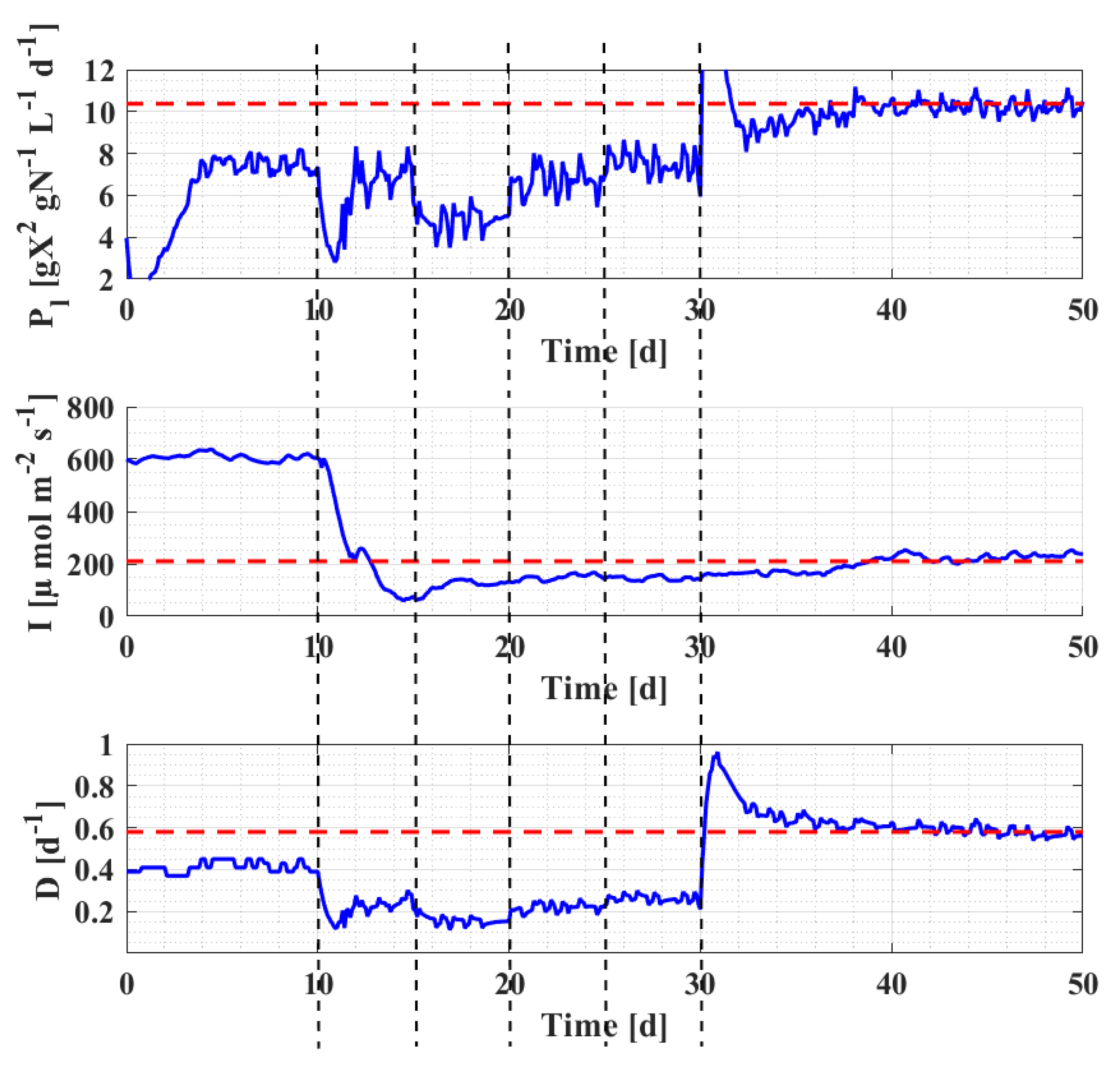
Figure 4 shows that the productivity reference trajectory (i.e., a succession of step changes) is well followed by the controller (see the evolution after 10 days of open-loop operation). The incident light intensity is set at the optimum, and its value quickly settles, whereas the dilution rate is varied so as to achieve the different productivity levels. In this figure, the blue dashed curves correspond to the suboptimal open-loop signals determined by the slope generator, while the black continuous lines represent the actual signals generated by the controller, which also include the PBRS dither signals. Figure 5 shows the phase plane plot evolution, while Figure 6 shows the gradient evolution.

Figure 7 confirms that PPC with integral action behaves as expected, the latter showing good performance during the transient phases despite the dependence on the estimate convergence and accuracy.

7. An Experimental Validation: Optimization of Micro-Algae Biomass Productivity

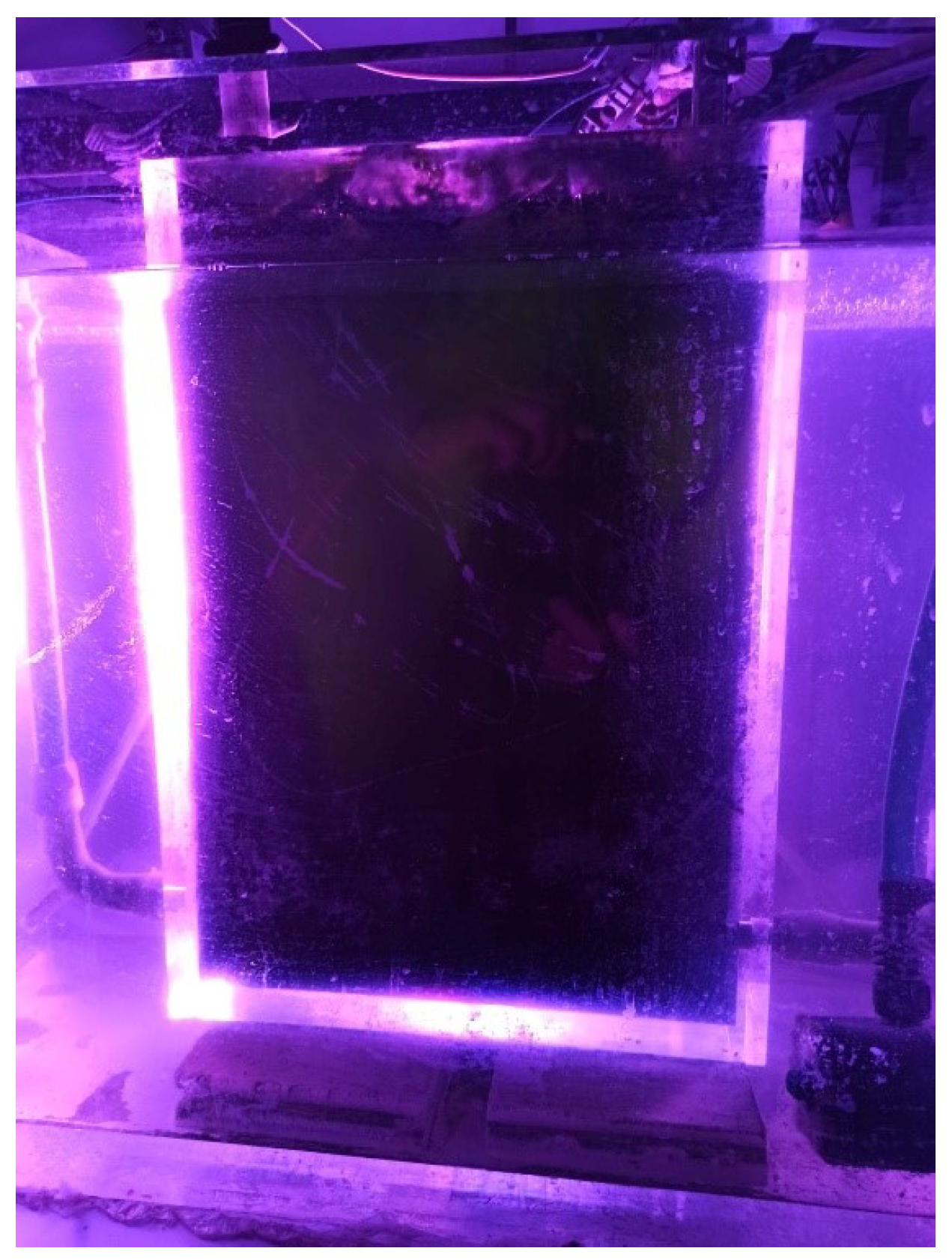
Figure 8 shows the lab-scale photobioreactor where the experiments are carried out to assess the performance of SSC. The PBR is equipped with several plunging probes for the online monitoring of the micro-algae concentration as well as the control of the temperature and pH of the medium. To optimize the homogeneity of the micro-algae culture, air-lift flows are achieved on both PBR sides. The PBR vessel is immersed in a water bath whose temperature is regulated by a chiller/heater and a pump that circulates the water to the chiller and back to the water bath. pH is regulated by injecting carbon dioxide. The incident light is generated by a horticultural light fixture with LED lights providing appropriate intensity for the micro-algae growth. Quantum sensors are used to measure the light intensity at the PBR surface, and a PI controller is designed to regulate the incident light intensity. To ensure a continuous mode operation, two peristaltic pumps control the inlet and outlet flows so as to achieve some required dilution rate. The control algorithm is implemented on a LabView platform for real-time computation, and Labjack cards are used for data acquisition.

To validate the slope-seeking control (SSC) in a practical setting, the dilution rate and light intensity are used as manipulated inputs, while the measurable productivity is considered as the performance index. It is therefore a simpler situation than the one considered in the previous simulation experiments. Here, there is no need to measure or estimate the internal quota Q, as it is not involved in the cost function. A sample experiment is described in what follows, which is conducted over 8.6 days, with a sampling period of $T_s=$ 0.1 d = 2.4 h.

After inoculation, the culture must first settle until biomass concentration reaches a steady-state corresponding to a constant dilution rate $D\left(0\right)=$ 0.1 d${}^{-1}$ and a constant average incident light $I_{av}=$ 500 $\mathsf{\mu }$E/(m${}^2$·s). The inlet substrate concentration is $S_{in}=$ 0.1 gN·L${}^{-1}$. Temperature and pH are kept constant, respectively, at 26 °C and 7.3. After the steady state has occurred (in this case for $X\left(0\right)=$ 0.88 gX·L${}^{-1}$), the slope seeking control is activated with a productivity setpoint of $P=$ 0.2 gX/(L·d). The dilution rate and incident light are then manipulated by the controller so as to achieve the desired level of productivity. After 7.6 days, the setpoint is changed to $P=$ 0.1 gX/(L·d) to challenge the tracking performance of the SSC. The time evolution of the several signals is shown in Figure 9 and Figure 10.

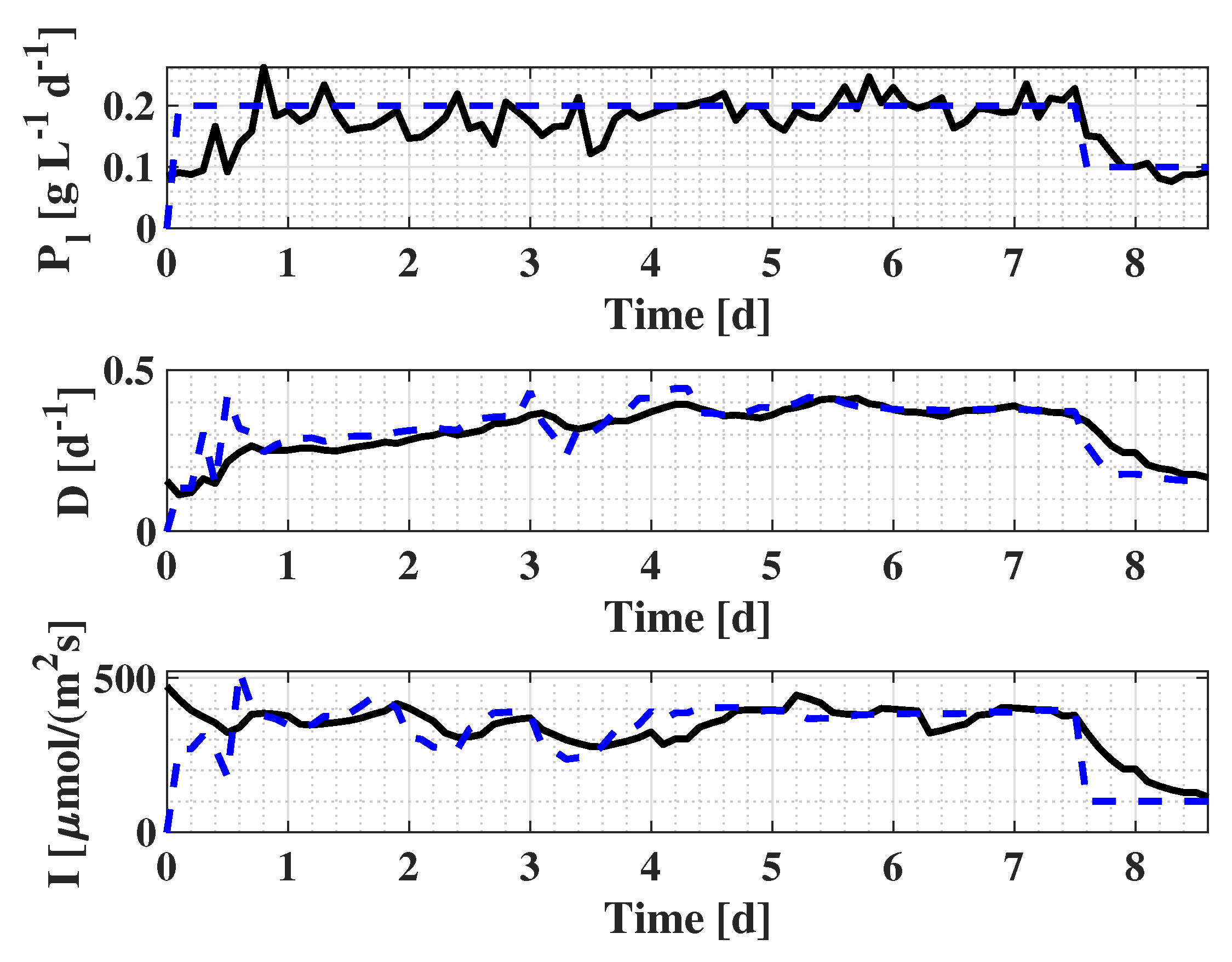
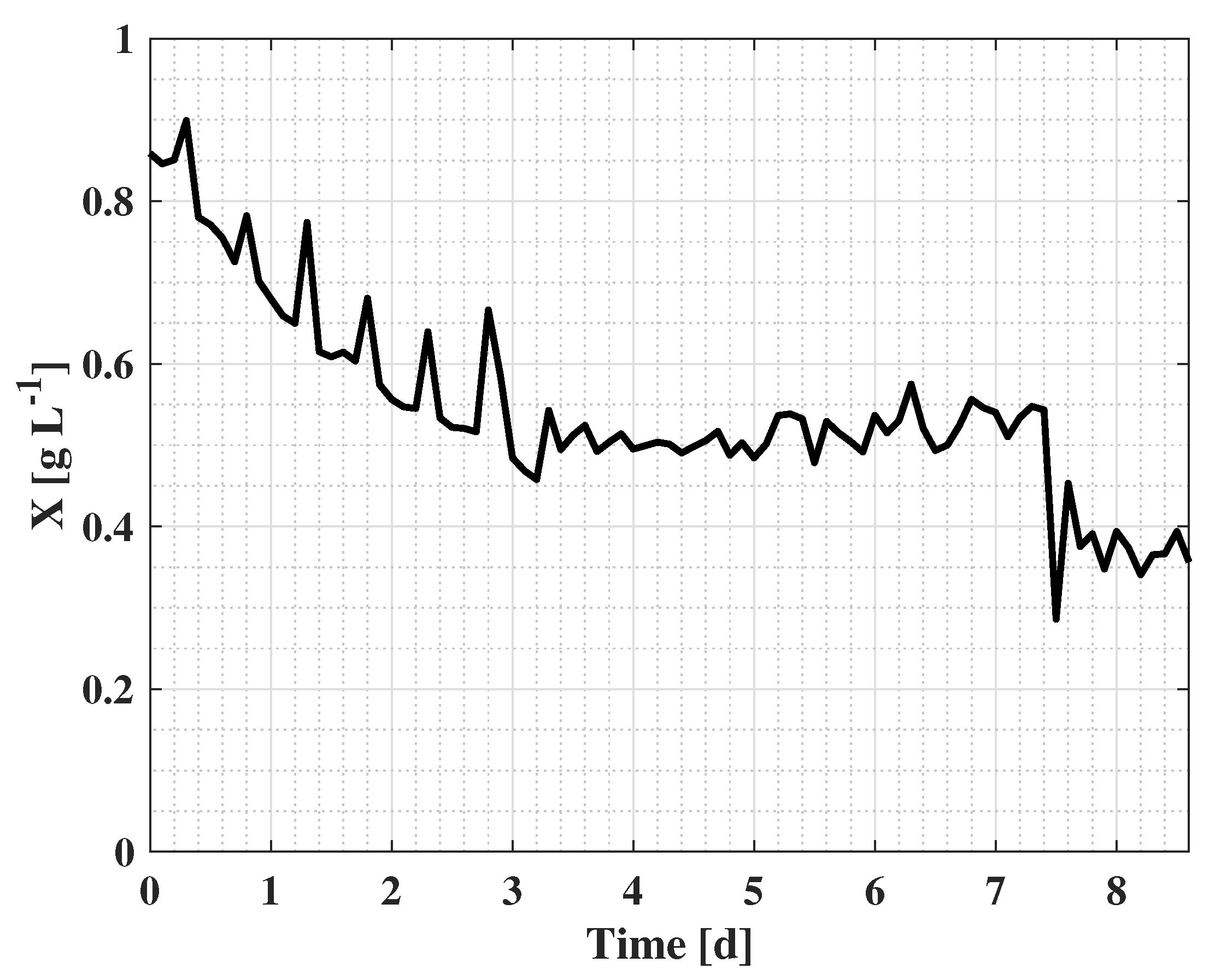
During the first phase, i.e., when the setpoint $P=$ 0.2 gX/(L·d) is imposed, the system converges within 1 day to the desired productivity level, but the steady-state is only truly established after 3 days, as shown by the biomass concentration evolution in Figure 10. The steady-state values of biomass, dilution rate, and incident light are, respectively, approximately $X=$ 0.5 gX/L, $D=$ 0.35 d${}^{-1}$ and $I=$ 380 $\mathsf{\mu }$E/(m${}^2$·s). When imposing the reference $P=$ 0.1 gX/(L·d), the new steady-state is achieved faster, i.e., within 1 day, and the corresponding values are $X=$ 0.39 gX/L, $D=$ 0.2 d${}^{-1}$ and $I=$ 150 $\mathsf{\mu }$E/(m${}^2$·s). This behavior can be explained by the fact that the RELS estimates need some time to converge when the first setpoint is imposed. The second setpoint can be achieved faster as the RELS estimation is probably close to the correct values and is able to track well the changes. We can only speculate about this observation as the values of the parameters are not known a priori.

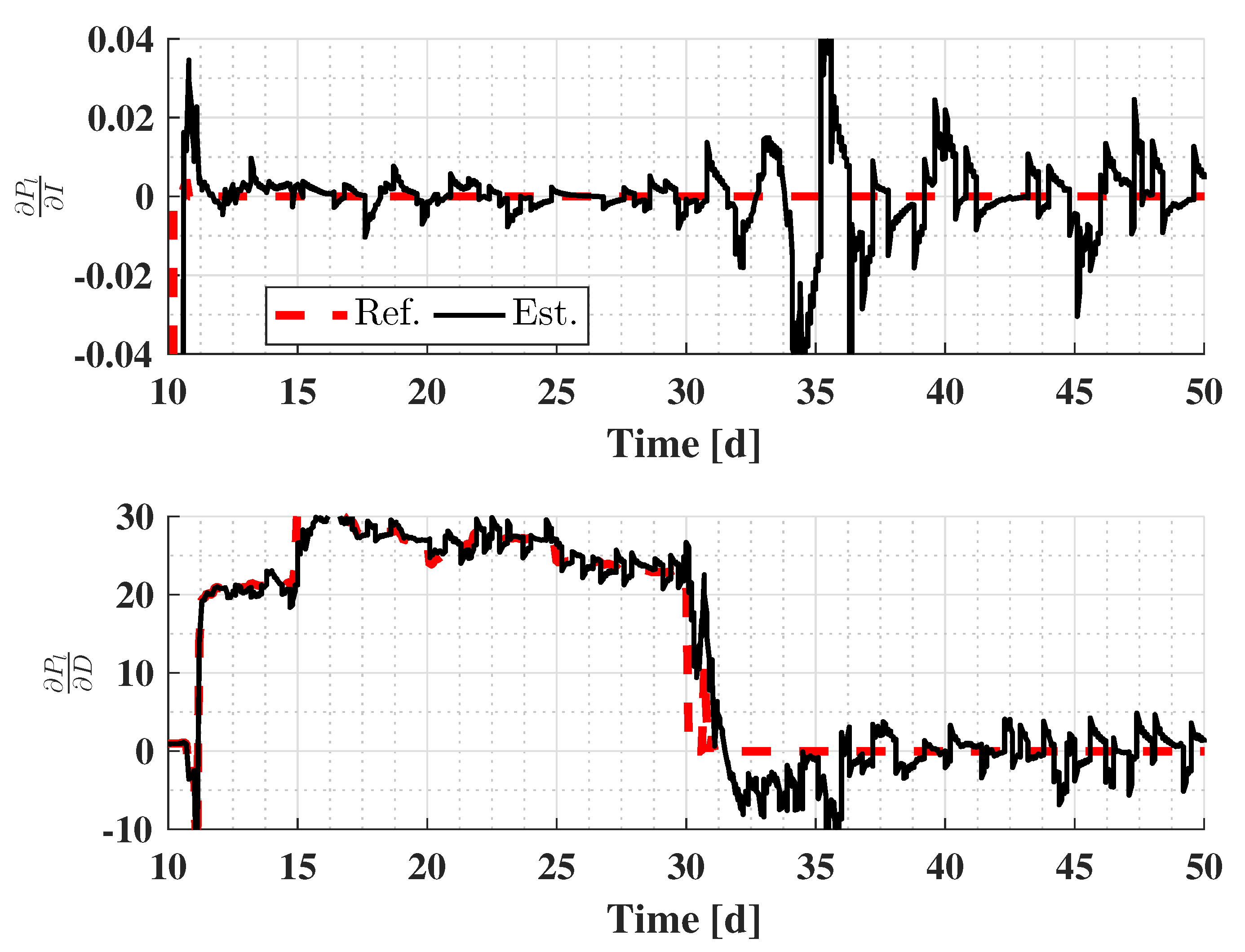
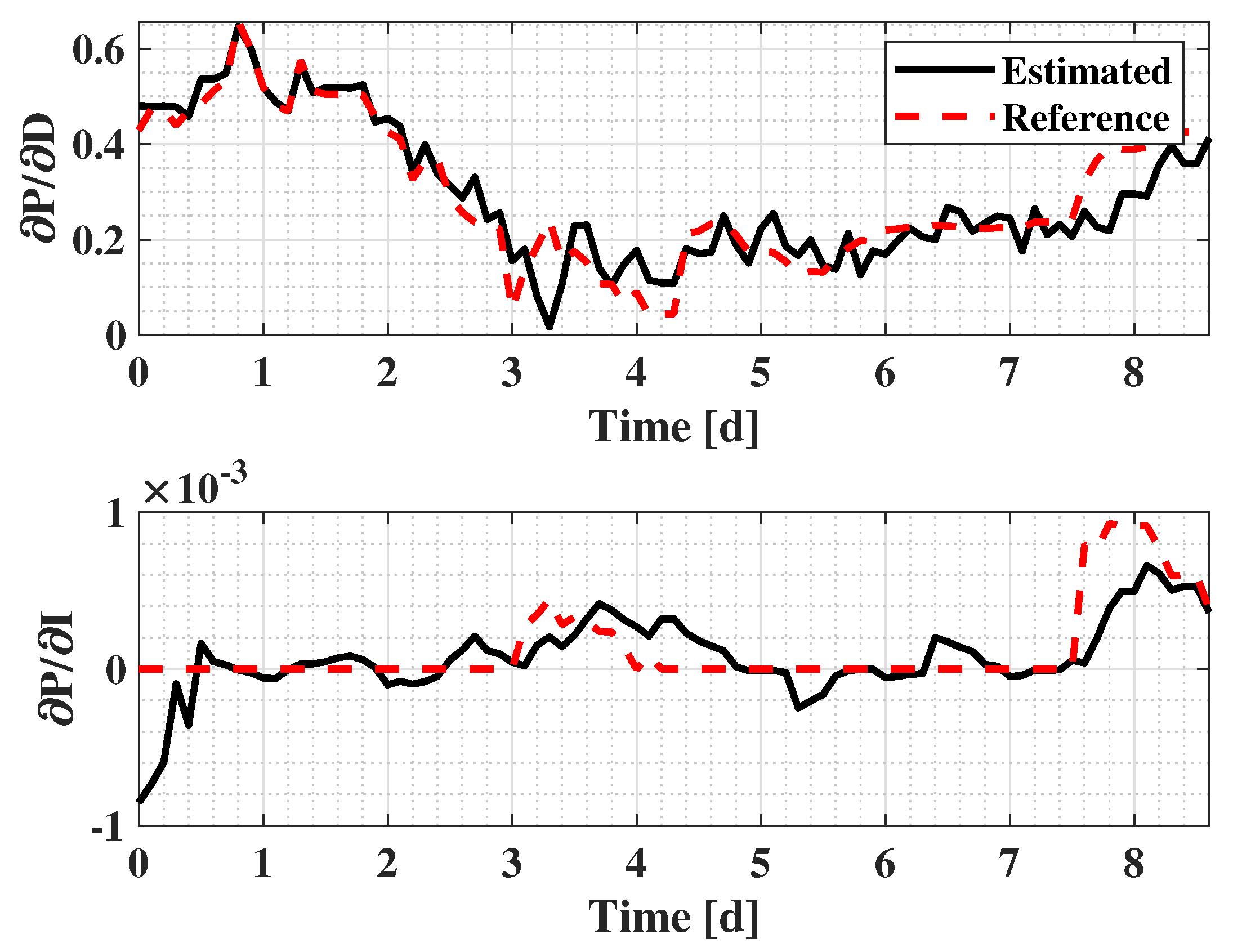
Figure 11 shows the evolution of the gradient components with respect to the dilution rate and light intensity. The latter is to be minimized, that is, pushed to zero, as shown in Figure 11, where this objective is achieved within 1 day and maintained despite some variations due to the slower convergence of the dilution rate component to 0.2 (comparable to the biomass convergence rate, that is, 3 days). Following the step change in productivity reference, the gradient experiences a sudden change, but the signal converges fast back to zero while the dilution component of the gradient reaches the new value of 0.4.

Regarding the application of the method in an industrial environment, a short practical guideline could be established, listing the steps to be achieved in the following order:

• Run first the extremum seeking (tracking a zero gradient) to determine the maximum achievable productivity level;
• Use the resulting productivity level as a reference to set achievable sub-optimal levels corresponding to non-zero slopes/gradients calculated by the controller;
• Sequentially reset the controller, setting new sub-optimal productivity levels until the desired operating conditions are met.

8. Conclusions

In this paper, an adaptive slope seeking strategy that allows extremum seeking control and suboptimal setpoint tracking for dual-input single-output processes is proposed. In this setup, the process is represented by Hammerstein models combining a quadratic static block with a second-order time-invariant dynamic block. A recursive extended least square algorithm is used to estimate the static map parameters in the presence of noisy measurements. Based on those estimates, 2 algorithms are provided for the generation of slope references, with the possibility of minimizing one or both inputs. The slope-seeking strategy is applied successfully in simulation to the optimization of the lipid productivity in continuous cultures of micro-algae in photobioreactors. Further, it was validated at a laboratory scale in experimental tests aiming at biomass productivity optimization. Further work might consider the extension of this scheme to situations with more than two inputs, paying particular attention to the selection of appropriate excitation signals.

References

- Chachuat, B.; Srinivasan, B.; Bonvin, D. Adaptation strategies for real-time optimization. Comput. Chem. Eng. 2009, 33, 1557–1567. [Google Scholar] [CrossRef]
- Ariyur, K.B.; Krstic, M. Real-Time Optimization by Extremum-Seeking Control; Wiley-Interscience ed.; John Wiley & Sons, Inc.: Hoboken, NJ, USA, 2003. [Google Scholar]
- Krstic, M.; Wang, H.H. Stability of Extremum Seeking Feedback for General Nonlinear Dynamic Systems. Automatica 2000, 36, 595–601. [Google Scholar] [CrossRef]
- Mustafa, A.; Morita, T. Efficiency optimization of rotary ultrasonic motors using extremum seeking control with current feedback. Sens. Actuators A Phys. 2019, 289, 26–33. [Google Scholar] [CrossRef]
- Kumar, S.; Mohammadi, A.; Gans, N.; Gregg, R.D. Automatic tuning of virtual constraint-based control algorithms for powered knee-ankle prostheses. In Proceedings of the 2017 IEEE Conference on Control Technology and Applications (CCTA), Maui, HI, USA, 27–30 August 2017; pp. 812–818. [Google Scholar]
- Dochain, D.; Perrier, M.; Guay, M. Extremum seeking control and its application to process and reaction systems: A survey. Math. Comput. Simul. 2011, 82, 369–380. [Google Scholar] [CrossRef]
- Guay, M.; Dochain, D. A proportional-integral extremum-seeking controller design technique. Automatica 2017, 77, 61–67. [Google Scholar] [CrossRef]
- Dewasme, L.; Srinivasan, B.; Perrier, M.; Vande Wouwer, A. Extremum-seeking algorithm design for fed-batch cultures of microorganisms with overflow metabolism. J. Process Control 2011, 21, 1092–1104. [Google Scholar] [CrossRef]
- Feudjio Letchindjio, C.G.; Deschenes, J.S.; Dewasme, L.; Vande Wouwer, A. Extremum seeking based on a Hammerstein-Wiener representation. IFAC-PapersOnLine 2018, 51, 744–749. [Google Scholar] [CrossRef]
- Giordano, G.; Gros, S.; Sjöberg, J. An improved method for Wiener–Hammerstein system identification based on the Fractional Approach. Automatica 2018, 94, 349–360. [Google Scholar] [CrossRef]
- Moase, W.H.; Manzie, C. Fast extremum-seeking on Hammerstein plants. IFAC Proc. Vol. 2011, 44, 108–113. [Google Scholar] [CrossRef] [Green Version]
- Ghaffari, A.; Seshagiri, S.; Krstić, M. Multivariable maximum power point tracking for photovoltaic micro-converters using extremum seeking. Control Eng. Pract. 2015, 35, 83–91. [Google Scholar] [CrossRef]
- Gelbert, G.; Moeck, J.P.; Paschereit, C.O.; King, R. Advanced algorithms for gradient estimation in one-and two-parameter extremum seeking controllers. J. Process Control 2012, 22, 700–709. [Google Scholar] [CrossRef]
- Ariyur, K.B.; Krstić, M. Slope seeking: A generalization of extremum seeking. Int. J. Adapt. Control Signal Process. 2004, 18, 1–22. [Google Scholar] [CrossRef]
- Feudjio Letchindjio, C.G.; Dewasme, L.; Deschênes, J.S.; Vande Wouwer, A. A slope seeking-based approach for optimal and sub-optimal SISO process control: Application to microalgae culture. IFAC-PapersOnLine 2019, 52, 370–375. [Google Scholar] [CrossRef]
- Feudjio Letchindjio, C.G.; Dewasme, L.; Deschênes, J.S.; Vande Wouwer, A. An extremum seeking strategy based on block-oriented models: Application to biomass productivity maximization in micro-algae cultures. Ind. Eng. Chem. Res. 2019, 58, 13481–13494. [Google Scholar] [CrossRef]
- Deschênes, J.S.; St-Onge, P.N.; Collin, J.C.; Tremblay, R. Extremum Seeking Control of Batch Cultures of Microalgae Nannochloropsis Oculata in Pre-Industrial Scale Photobioreactors. IFAC Proc. Vol. 2012, 45, 585–590. [Google Scholar] [CrossRef]
- Tebbani, S.; Lopes, F.; Filali, R.; Dumur, D.; Pareau, D. Nonlinear predictive control for maximization of CO2 bio-fixation by microalgae in a photobioreactor. Bioprocess Biosyst. Eng. 2014, 37, 83–97. [Google Scholar] [CrossRef] [PubMed]
- Tebbani, S.; Filali, R.; Lopes, F.; Dumur, D.; Pareau, D. Biofixation by Microalgae: Modeling, Estimation and Control; Wiley & Sons: Hoboken, NJ, USA, 2014. [Google Scholar]
- Ifrim, G.; Titica, M.; Barbu, M.; Ceanga, E.; Caraman, S. Optimization of a Microalgae Growth Process in Photobioreactors. IFAC PapersOnLine 2016, 49, 218–223. [Google Scholar] [CrossRef]
- Torres, I.; López-Caamal, F.; Hernández-Escoto, H.; Vargas, A. Extremum seeking control based on the super-twisting algorithm. IFAC PapersOnLine 2020, 53, 1621–1626. [Google Scholar] [CrossRef]
- Giri, F.; Bai, E.W. Block-Oriented Nonlinear System Identification; Springer: Berlin/Heidelberg, Germany, 2010; Volume 1. [Google Scholar]
- Wang, H.H.; Krstic, M.; Bastin, G. Optimizing Bioreactors by Extremum-seeking. Int. J. Adapt. Control Signal Process. 1999, 13, 651–669. [Google Scholar] [CrossRef]
- Dewasme, L.; Vande Wouwer, A. Model-Free Extremum Seeking Control of Bioprocesses: A Review with a Worked Example. Processes 2020, 8, 1209. [Google Scholar] [CrossRef]
- Forssell, U.; Ljung, L. Closed-loop identification revisited. Automatica 1999, 35, 1215–1241. [Google Scholar] [CrossRef] [Green Version]
- Gustavsson, I.; Ljung, L.; Söderström, T. Identification of processes in closed loop identifiability and accuracy aspects. Automatica 1977, 13, 59–75. [Google Scholar] [CrossRef] [Green Version]
- Tan, Y.; Nesic, D.; Mareels, I.; Astolfi, A. On Global Extremum Seeking in the Presence of Local Extrema. Automatica 2009, 45, 245–251. [Google Scholar] [CrossRef]
- Choi, J.Y.; Krstic, M.; Ariyur, K.B.; Lee, J.S. Extremum seeking control for discrete-time systems. IEEE Trans. Autom. Control 2002, 47, 318–323. [Google Scholar] [CrossRef] [Green Version]
- Ghaffari, A.; Krstić, M.; Nešić, D. Multivariable Newton-based extremum seeking. Automatica 2012, 48, 1759–1767. [Google Scholar] [CrossRef]
- Yin, C.; Wu, S.; Zhou, S.; Cao, J.; Huang, X.; Cheng, Y. Design and stability analysis of multivariate extremum seeking with Newton method. J. Frankl. Inst. 2018, 355, 1559–1578. [Google Scholar] [CrossRef]
- Landau, I.D.; Lozano, R.; M’Saad, M.; Karimi, A. Adaptive Control: Algorithms, Analysis and Applications; Springer Science & Business Media: New York, NY, USA, 2011. [Google Scholar]
- Goodwin, G.C.; Sin, K.S. Adaptive Filtering Prediction and Control; Courier Corporation: North Chelmsford, MA, USA, 2014. [Google Scholar]
- Nelles, O. Nonlinear System Identification: From Classical Approaches to Neural Networks and Fuzzy Models; Springer Science & Business Media: New York, NY, USA, 2013. [Google Scholar]
- Braun, M.; Rivera, D.; Stenman, A.; Foslien, W.; Hrenya, C. Multi-level pseudo-random signal design and “model-on-demand” estimation applied to nonlinear identification of a RTP wafer reactor. In Proceedings of the 1999 American Control Conference (Cat. No. 99CH36251), San Diego, CA, USA, 2–4 June 1999; Volume 3, pp. 1573–1577. [Google Scholar]
- Ljung, L. System Identification: Theory for the User; Prentice-Hall: Upper Saddle River, NJ, USA, 1987. [Google Scholar]
- Åström, K.; Wittenmark, B. Adaptive Control; Addison-Wesley Publishing Company: Reading, MA, USA, 1995. [Google Scholar]
- Droop, M. Vitamin B12 and marine ecology. IV. The kinetics of uptake, growth and inhibition in Monochrysis lutheri. J. Mar. Biol. Assoc. UK 1968, 48, 689–733. [Google Scholar] [CrossRef]
- Bernard, O.; Rémond, B. Validation of a simple model accounting for light and temperature effect on microalgal growth. Bioresour. Technol. 2012, 123, 520–527. [Google Scholar] [CrossRef]
- Bernard, O. Hurdles and challenges for modelling and control of microalgae for CO2 mitigation and biofuel production. J. Process Control 2011, 21, 1378–1389. [Google Scholar] [CrossRef]
- Sati, H.; Mitra, M.; Mishra, S.; Baredar, P. Microalgal lipid extraction strategies for biodiesel production: A review. Algal Res. 2019, 38, 101413. [Google Scholar] [CrossRef]
- Feudjio Letchindjio, C.G.; Dewasme, L.; Vande Wouwer, A. Extremum-Seeking for micro-algae biomass productivity maximization: An experimental validation. IFAC-PapersOnLine 2019, 52, 281–286. [Google Scholar] [CrossRef]
- Coutinho, D.; Vargas, A.; Feudjio Letchindjio, C.; Benavides, M.; Vande Wouwer, A. A robust approach to the design of super-twisting observers–application to monitoring microalgae cultures in photo-bioreactors. Comput. Chem. Eng. 2019, 121, 46–56. [Google Scholar] [CrossRef]
Figure 1.
Illustration of the DISO adaptive slope seeking scheme.
Figure 2.
Steady-state productivity maps with respect to dilution rate
D and incident light
I. Red ‘*’: Optimal values using
P (
32) and Blue ’*’: Optimal values using
(
33).
Figure 3.
Time evolution of Q, , and in black and their estimates provided by the AO and the 2 RELS in blue.
Figure 4.
Time evolution of productivity , incident light I, and dilution rate D following SOP and ESC (red: optimal values; blue: estimated references; black: trajectory; magenta: ).
Figure 5.
Level lines of the performance index in the plane and corresponding productivity .
Figure 6.
Time evolution of the estimated gradient and .
Figure 7.
PPC controller performance: Time evolution of productivity , incident light I, and dilution rate D following SOP and ESC (red: optimal values; solid blue: PPC; The SOC step changes are indicated by the vertical dashed lines.
Figure 8.
Lab-scale flat-panel photobioreactor.
Figure 9.
Time evolution of productivity, dilution rate and light intensity during the experimental validation of the SSC method. Dashed lines, calculated references; continuous lines, measured productivity and SSC computed inputs.
Figure 10.
Time evolution of the algal biomass during the experimental validation of the SSC method.
Figure 11.
Time evolution of the gradient components during the experimental validation of the SSC method. Dashed lines, calculated references; continuous lines, SSC estimates.