1. Introduction
The visual measurement of velocity profile distribution in silt carrying flow is a basic job before river engineering tests for solving actual water-related sediment-laden problems, one which has challenged scientists and hydraulic engineers for a long time [
1,
2,
3]. The real-time analysis of flow dynamic structure with quantitative and multidimensional information plays a vital part in solving many complicated spatial velocity distribution and turbulence problems [
4,
5,
6]. These problems enable us to study other vorticity and deformation conditions, which are key to researching flow structures and hydrodynamics [
7,
8,
9]. Traditional instruments are mostly point-to-point measurement modes, such as some laser-Doppler and hot-wire anemometers. They cannot reveal the profile velocity and its spatial distribution structure of sediment-laden flow at the same time. With the traditional Doppler device exists the angulation error problem with the measured velocity component just along the ultrasound beam, limiting the real-time analysis of spatial velocity vector. Therefore, the traditional Doppler device requires the parallel alignment of the ultrasound beam to the silt carrying flow direction.
The optical particle image velocimetry (PIV) technique is widely used in image measurement [
10,
11,
12]. It is a reliable method and allows us to obtain quantitative information, including water flow spatial structures [
13,
14,
15]. However, the well-known limitation of the optical measuring principle is that optical methods can only be feasible for transparent fluids through which optical light can pass. These limit their further applications in some opaque objects, such as suspensions and silt carrying flow. Recent PIV applications where these limitations are partially overcome include the use of granular PIV (g-PIV) exploit flash or LED lamps to obtain reliable near-wall velocity measurements of granular flows and liquid–granular mixtures [
16,
17,
18]. Still, the setup may be too complex for a portable device during the application.
To overcome these disadvantages and meet the requirement of the field velocity measurement of silt carrying flow, a visual and real-time measurement method of velocity profile distribution by using an ultrasound PIV system and iterative multi-grid deformation technique was developed [
19], referred to as an improved ultrasound imaging device and a novel algorithm. The operating protocol for the ultrasound PIV system is composed of a medical ultrasound machine with a PIV algorithm and an interface program. This approach is appropriate for real-time measurement of velocity profile distribution in silt carrying flow condition by combining the ultrasound imaging technique with the digital PIV method [
20]. The main advantage of the ultrasound PIV system compared with some Doppler-based techniques is that all the velocity components, both perpendicular and parallel to the ultrasound beam, can also be measured. Therefore, it can improve its accuracy, simplicity, and accessibility without some Doppler-based limitations [
21].
For spatial velocity measurements in silt carrying flow or through optical image methods, the ultrasound PIV method is a promising technique to obtain two-dimensional flow fields and velocity profile distribution [
22]; hence, this method can conduct a quantitative performance assessment through actual ultrasonic images obtained in a seeded flow. The method can improve the accuracy of the particle image displacement at a sub-pixel level. On the one hand, velocity profile distribution fields within the laminar flow field measured using the ultrasound PIV method are in excellent agreement with analytical profiles [
23,
24,
25]. On the other hand, the ultrasound imaging process is different from Optical PIV, which is acquired line-by-line through the view field sequentially, so its performance could be further improved using sweep correction.
In the near-wall surface layer, the flow velocity field profile shows a strong gradient. The silt carrying flow refers to a sediment-laden flow with a suspended sediment concentration from 0.0001% to 0.5% in terms of the solid volume fraction during the physical model test [
12,
14]. In order to improve the silt carrying flow measurement accuracy and efficiency in regions with high-velocity gradients, this paper presents a new method for applying an improved ultrasound PIV system. The processing method of this system, including a window offsetting and iterative scheme, is used to increase the spatial resolution of flow velocity measurement to a maximum. To verify the feasibility of the ultrasound PIV system and the improved iterative multi-grid deformation technique, an experiment has also been conducted.
2. Ultrasound PIV System and Its Principle
The ultrasound PIV system mainly contains an ultrasound imaging device, two probes, an interface program, and a related physical model. The two probes are convex array or linear array, which are used to connect to the host machine of the ultrasound imaging device. They are used to generate a 2D ultrasonic image by pulsing the array elements in the probe at different times [
26,
27]. Each array element transmits an ultrasonic pulse into the flow, and sand particles in the flow can reflect ultrasonic echoes to the array elements where they can be recorded [
28]. The amplitudes of the reflected ultrasonic echoes and transmission time delays are used to create a series of ultrasonic images [
29,
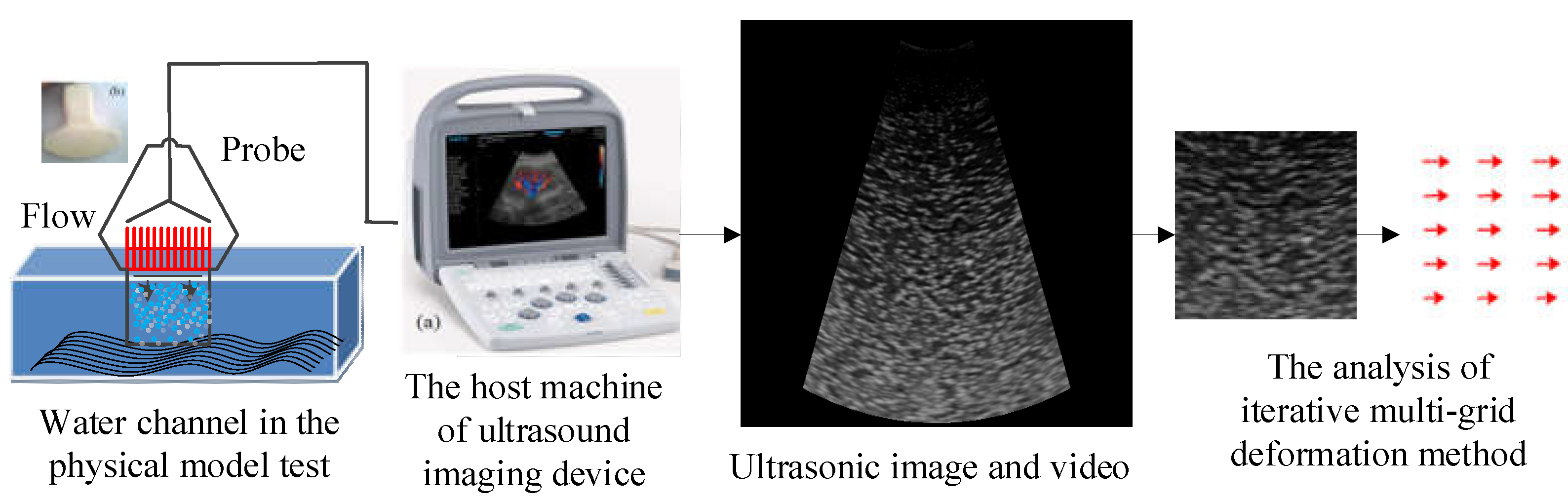
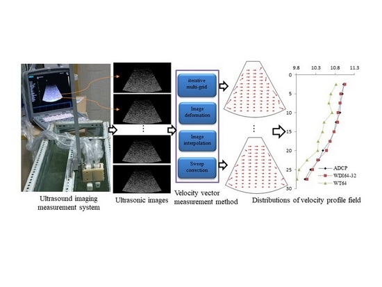
30]. The time delays are used to determine the spatial position of the sand particles in the flow, and the amplitudes are used to assign the reflected intensity of the particles. To obtain the ultrasonic image, the needed time is determined by the convex array probe when it has finished the transmission and reflection of all array elements. The acquisition and analysis process of the ultrasonic image is shown in
Figure 1. Then, these ultrasonic images are used to analyze and calculate the flow velocity vectors in silt carrying flow through the interface program.
Just as with optical PIV methods, the measuring principle of the ultrasound PIV system is also based on the basic principle of cross-correlation shown in
Figure 2. The number of pixels in the ultrasonic image is generally smaller than in the optical image, so the spatial resolution should be increased. As for the limitation of the ultrasound PIV system when applied to flow velocity measurement, the dynamic range of ultrasonic waves is the primary limitation. The frame rate of the formed ultrasonic image also has the limitation of image acquisition speed because of needing more time to generate high-resolution ultrasonic images for the device when compared with the optical PIV method. Therefore, higher frame rates and higher image resolution systems can be more available, and the actual application can be more accurate and welcome. In this paper, an improved measurement system that can enhance the measured accuracy of ultrasonic images is described [
31] and provides a novel method based on the cross-correlation principle through discrete window offset [
32]. This approach can make full use of the deformation of the interrogation window and rebuild this translation by reconsidering the rotation and shear of imaging particles. The displacement and detected offset in the ultrasonic image can be obtained and corrected using some iterative steps through the multi-grid deformation technique.
3. Flow Velocity Measurement Method
3.1. Main Steps of the Method
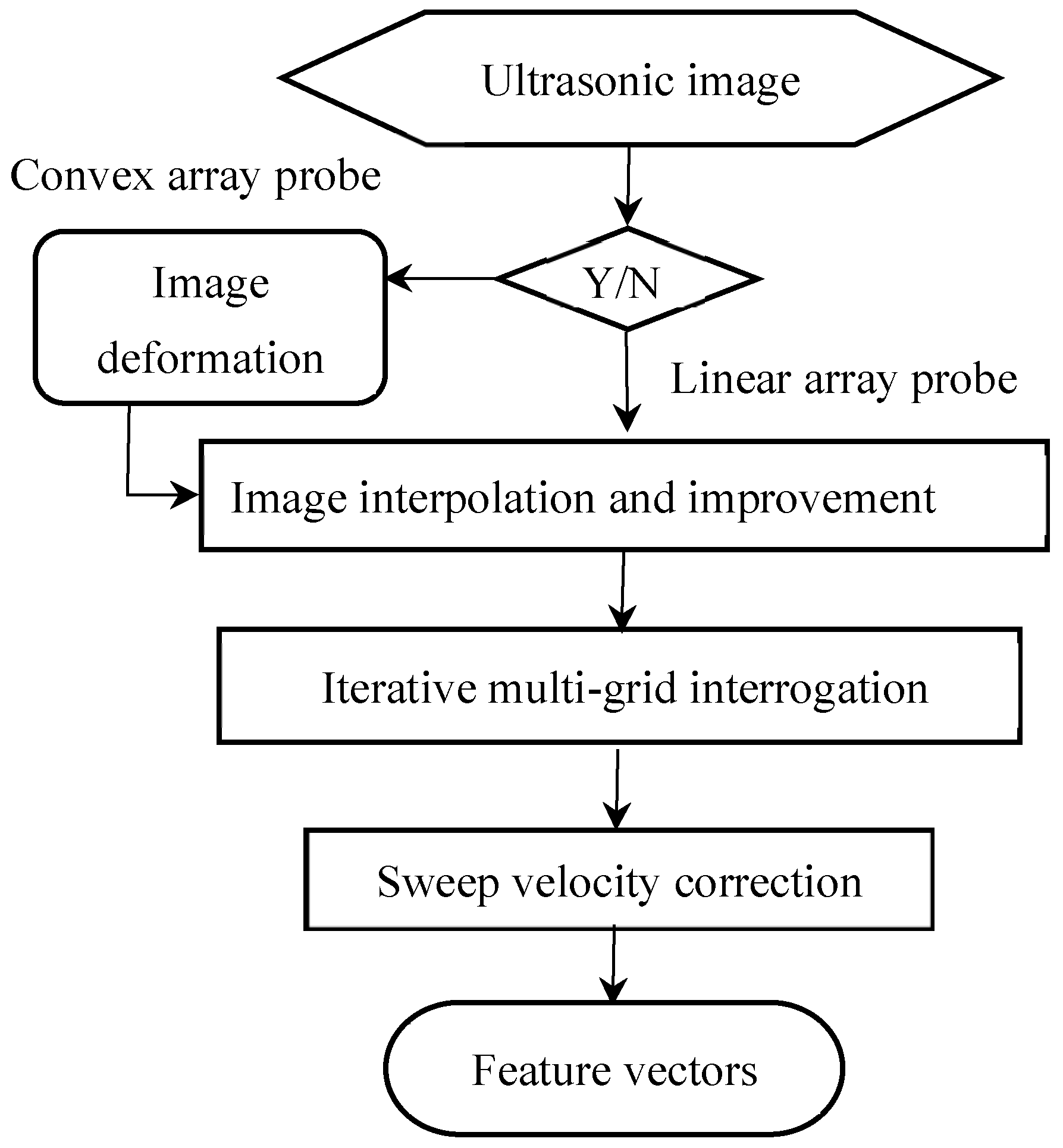
To obtain the accurate velocity profile field, we take an iterative multi-grid deformation technique to process and analyze the ultrasonic images, which are obtained by using the above ultrasound PIV system in silt carrying flow. The main steps of the flow velocity measurement method are shown in
Figure 3. This method can improve the spatial resolution and detecting speed compared with traditional ultrasound PIV methods.
Among the steps, the image deformation should be used for an image correction when a convex array probe is used during the physical model test. This step can be skipped if a linear array probe is used because the imaging of the linear array probe is nearly rectangular without deformation. The step of image interpolation and improvement is necessary before calculating image features because the image size is relatively small. The most important step of iterative multi-grid interrogation is to realize the measurement of flow velocity by calculating the feature vector in the ultrasonic image. The basic principle of this step is based on an image cross-correlation algorithm. After the feature vector is calculated, the vector should be recorrected because it has a relationship with the sweep velocity of the ultrasound probe. Therefore, sweep velocity correction is a revised method to obtain the real flow velocity.
3.2. The Principle of Main Steps and Analysis
3.2.1. Image Deformation
When the convex array probe of the ultrasound imaging device is used for detecting flow during the physical model test, the imaging of silt carry flow is a kind of conformal mapping from an arc-annular shape. Therefore, image deformation is necessary for the correction of flow imaging information. The imaging of the flow by using the ultrasound imaging device always is an annular conformal mapping within a certain angle, even though it uses the linear array probe. In order to create an accurate reconstruction of the velocity field, we converted the arc-annular shape into a rectangular shape using the convex array probe for a better feature match of overlapping sub-images.
When we want to obtain the flow velocity, the displacement of imaging particle in the image is the key according to the normal PIV method, and the displacement can be detected by using a cross-correlation function under the assumption that the particles’ motion in the interrogation window of the image is almost regular. However, this assumption is hardly valid in practice. The velocity profile vector shows an obvious change within the interrogation window in the silt carrying flow. The cross-correlation peak and different velocities produced by image pairs will become larger, as shown in
Figure 2, which may be split into multiple cross-correlation peaks as a result of the large differences of particle velocity across the window during some extreme conditions. Therefore, the calculation of velocity profile can be affected when the velocity gradient is large and may suffer from a much higher velocity vector rejection rate. Because of this, we take an iterative window deformation technique to compensate for the effect of peak broadening and the gradient difference of in-plane velocity. This approach can improve results of image matching when two adjacent ultrasonic images are deformed iteratively according to the flow velocity field [
33]. The main advantage of the image deformation is the added robustness and accuracy. It can improve the effect of sub-image match, especially for highly sheared flows when compared to the discrete window offset method. The basic principle of this process is shown in
Figure 4.
We use a spatial cross-correlation function for the deformed images in this paper compared with the standard cross-correlation function. The equation is defined as:
while
and
denote the image intensity, which is reconstructed after image deformation by using the predicted deformation displacement field
in a central difference process, shown as Formula (2):
The deformation displacement field
is a spatial distribution without a uniform condition. Therefore, smooth interpolation at each pixel in the ultrasonic image is required. In a steady condition of the flow, the first-order term of the Taylor series is enough for the image reconstruction by using local displacement, which can be shown as Formula (3):
where
x0 is the center position of the interrogation window. The smooth interpolation can be described as follows.
3.2.2. Image Interpolation and Improvement
The displacement field may change at times. The image intensity
must translate floating-point types because of interpolating non-integer values, which will increase computational cost. Image interpolation has been widely used in image processing, but an ultrasonic image needs many kinds of interpolation ways for the velocity measurement based on the PIV method. A concise comparison of many advanced image interpolators used for PIV image deformation schemes can be found in [
4,
17,
21,
31,
33]. Because the interpolator of the ultrasonic image should reconstruct steep intensity gradients in the particle image in the first place, we used the B-splines method to balance the computational cost and the performance. Results show that the deviation from the actual displacement is only one-fifth per pixel. If higher accuracy and precision are required, the sinc-based interpolation method [
34], such as the Whittaker reconstruction and the FFT-based interpolation algorithm, should be utilized by using many points. However, the computational cost may be increased if an unsuitable approach is taken according to [
35].
3.2.3. Iterative Multi-Grid Interrogation
The analysis process of ultrasonic images includes multi-grid analysis and iterative PIV interrogation analysis. The interrogation window size is gradually decreased when the cross-correlation is applied during the multi-grid analysis process. It can eliminate some rule constraints, usually terminated when the desired window size (8 × 8) is applied. Iterative PIV interrogation analysis can further improve the accuracy of PIV image deformation and enhance spatial resolution. The whole process will be terminated when the required incremental change is applied.
The iterative PIV interrogation analysis process can be described as a predictor-corrector process and shown as the following formula:
where
is the evaluated result of the
k-th iteration and
is the correction term, which can be described as the residual displacement. Using a central difference function to calculate the deformed ultrasonic image and interrogating several times obtains a more accurate displacement field. In practice, two or three iterations have been enough to obtain a converged result, because most in-plane imaging particle motions can be compensated effectively through image deformation. The spatial resolution of the image after iterative analysis can be higher than twice the discrete or single-step window-shift algorithm.
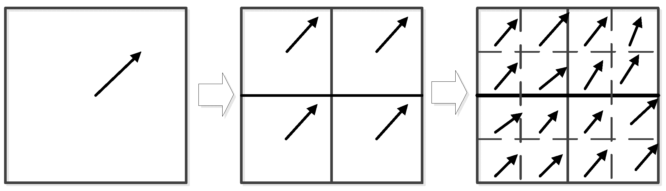
Therefore, the iterative multi-grid interrogation process can be improved by using a hierarchical approach. The sampling grid of the algorithm can be refined continually. At the same time, the size of the interrogation window can be decreased simultaneously, which can improve the capability of interrogation window sizes by using smaller particle image displacement. This process can increase the dynamic spatial range. It is especially useful for the pretreatment of ultrasonic images with both higher particle image density and a higher dynamic range in the displacements and detected offsets. The basic principle of the iterative multi-grid interrogation process can be shown in
Figure 5. The line arrow presents the direction of the flow in the box. The box is divided from one to four and then to sixteen, which means that the direction of the flow becomes more precise and clearer.
Additionally, particle image density can affect the choice of the final interrogation window size. When the particle image density or the number of particles decreases to a certain extent in the targeted interrogation window, the detection rate will decrease rapidly. The detecting speed, that is, the calculated feature vector, may be increased significantly by downsampling the image during the initial interrogation process at the same time. It can be realized by merging neighboring pixels by using the sum of N × N block pixels. This process can help the detection process become much faster when using interrogation samples [
36].
3.2.4. Sweep Velocity Correction
As the optical image is obtained by a snapshot of the CCD device for the optical PIV method, while the ultrasonic image is constructed by series of scanning lines for the ultrasound PIV system, the image forming time is the main difference. This means that different parts in the image are recorded and formed at different times. As is known, the velocity displacement in the optical image is formed by a time interval between snapshot frames. The time interval is also a displacement function. When particles move with a lateral velocity that becomes close to the ultrasound probe’s sweep velocity, the sweep velocity approaches the next scan line. Therefore, this sweep velocity can be corrected according to the frame rate and the lateral size of the view field according to the Doppler effect of flow velocity.
According to the ultrasound imaging principle and researchers’ discussion, the ultrasound beam sweeping effect can make some measuring errors [
37] and can affect the particle’s velocity in silt carrying flow. When the sweeping direction of the ultrasound beam is the same as the direction of the water flow, the measured velocity may be overestimated. Otherwise, the measured velocity may be underestimated. The ratio between sweep speed and flow speed also has some influence on the measuring results. If the ratio increases, the measuring error will decrease. Therefore, the imaging particle velocity obtained by this ultrasound PIV method can be re-corrected from the beam sweep effect by using the following formulas [
20]:
where
and
are the re-corrected velocity components,
and
are the uncorrected velocity components, and
is the sweep velocity of the ultrasound beam. Lastly, we can obtain a real particle velocity after this correction.
3.3. The Implementation Steps of Measuring Particle Velocity
The implementation steps of the particle velocity measuring process for the ultrasonic image during actual application can be summarized as follows:
Step 1: begin with a large interrogation sample to obtain the whole dynamic range of the displacement and then perform a standard interrogation process.
Step 2: obtain an initial displacement complying with the one-quarter rule, which means that the box is divided from one to four.
Step 3: replace incorrect data of the velocity vector field by using local mean and low-pass filtering methods. A filter kernel with the same window size is enough to smooth spurious emission and then suppress fluctuations by using a moving average filter.
Step 4: detect the extremums and repeat them by initial interpolation results. The newly detected displacements are used to obtain a higher resolution for the next step, so the criterion of extremum detection is more stringent than before.
Step 5: deform the recordings according to the filtered velocity vector field.
Step 6: pass interrogation on the deformed image within the interrogation window using the cross-correlation function and add the corrected result of the cross-correlation function to the filtered velocity profile field.
Step 7: project the detected displacements, that is, velocity, on the next higher level. Offset the interrogation windows by using the displacements.
Step 8: inspect the velocity vector field for extremums and replace them with interpolation.
Step 9: put an interrogation at the targeted sampling and interrogation window size, which is without extremum removing and smoothing.
Step 10: increase the resolution of the next level and repeat the above step about three times until the resolution of the actual ultrasonic image is reached. The increment of displacement will decrease gradually, along with the iterative number increasing. Lastly, the best displacement can be obtained and can be calculated as the detected feature vector.
Step 11: recorrect the obtained vector according to Formulas (5) and (6), translate it to flow velocity, and calculate the velocity profile distribution of the flow field.
Step 12: recalculate the vector with certain pixel distances by the depth-averaged approach and put the vector on the interrogation window. If further resizing the search region of the desired correlation peak, the final obtained velocity’s spatial resolution could be further improved.
4. Physical Model Experiments and Measuring Results
In order to verify and analyze the ultrasound PIV method and the iterative multi-grid deformation technique, we built a physical model system and carried out a series of experiments for the real-time measurement of velocity profile distribution. The schematic diagram of the ultrasound PIV measurement system is shown in
Figure 6, and its physical model system for all physical model experiments is shown in
Figure 7. Additionally, the measured velocities during the experiments are compared point-by-point with those of the acoustic Doppler current profilers (ADCP), and then the root mean square (RMS) error and average fluctuating velocity during the same experiments are analyzed.
The physical model of the ultrasound PIV measurement system mainly includes a medical ultrasound machine (hardware) and an interface program including an inside improved PIV method (software). The steady flow of a fluid in a long glass channel with circulating water flow is shown in
Figure 6. The size of the glass channel is 5.0 m × 1.2 m × 1.0 m (length × width × height). A convex or linear array probe with a frequency of 3.5 MHz is linked to the medical ultrasound machine. The frequency of ultrasonic waves from the probe can be 1 MHz, 2 MHz, 3.5 MHz, or 5 MHz. Higher frequency of the ultrasonic wave can improve the imaging precision of sediment-laden particles, but the detecting distance of the probe in silt carrying flow may be shorter. Therefore, we used a frequency 3.5 MHz probe during the model test. This system is installed near the water’s surface of a circulating water channel. The ultrasound imaging region is about 35 cm × 35 cm, which can be monitored by the array probe of the ultrasound system. Usually, the reliable depth of the measurement can be from 5 cm to 35 cm, and the measuring results can be shown directly in real-time. The array elements’ imaging direction of the probe should stay in the same direction as the main flow. The probe is fixed in the water channel and primarily measures particles in the water flow as they move across the imaging area of the probe. The circulating water channel has a pump, which is used to maintain a steady flow with a fixed voltage during the whole experiment. The ultrasound system can obtain a series of ultrasonic images with a size of 640 × 480 pixels. The spatial resolution of the ultrasonic image is about 32 × 32 pixel/cm
2. The frame rate of the ultrasound system can be up to 60 frames/s. Some key properties and specifications of the experimental device are shown in
Table 1.
The processing software includes some PIV codes that can be referred to as the built-in software of the ultrasound imaging device, and the program of the PIV method is on the website. The software should include the following main features: (1) it can link a personal computer to the ultrasound imaging device directly by using a high-speed network card; (2) it can real-time display the ultrasound imaging results of silt carrying flow within sand particles in the personal computer; (3) it can real-time transform and process the image video by editing the interface program; (4) it can calculate the vector map and analyze flow field and depth-averaged velocity distribution by using the iterative multi-grid deformation technique and the related ultrasound PIV method. The program of our used ultrasound imaging measurement system is a piece of software specially designed for our research. The experiments on the real-time measurement of velocity profile distribution in silt carrying flow were carried out on the physical model system shown in
Figure 7. The ultrasonic images are obtained by using the ultrasound PIV measurement system and the iterative multi-grid deformation technique. We took measurements with the convex array probe and the obtained original ultrasonic image is saved as 640 × 480, which is generally smaller than in optical PIV. Two consecutive frames are shown in
Figure 8, and the measurement results are shown in
Table 2 and
Figure 9 by using the interface program directly. Some descriptions of abbreviations are shown in
Table A1.
5. Analysis of Velocity Profile Distribution
In order to analyze and verify the measurement results, we should compare the measured results by keeping the same condition at different times and using the statistical average to replace the water velocity in a certain short time, because it is impossible to reproduce an identical flow field in practice simultaneously. We used the iterative multi-grid deformation technique to obtain the imaging particles’ displacement or feature vector and translate the value to the measured flow velocity. The average velocity is statistically obtained by 50 sequential ultrasonic images, and the flow field is represented by the mean velocity in a certain area. Velocity profile distribution is obtained from the velocity flow field by averaging velocity value and depth direction for a certain range in each profile field. Lastly, we analyzed the whole line averages from the 50 flow fields.
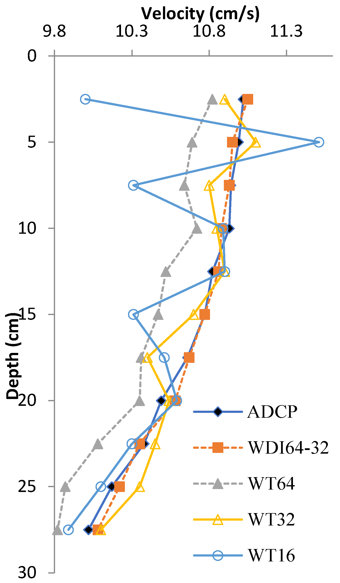
Additionally, the actual velocity profile distribution can be obtained using the ADCP method after a kind of experiment in the steady flow condition. The measured velocities of the ADCP method can be taken as the standard velocity and then compared with the results from our ultrasound PIV method. This is a suitable way to prove the velocity profile vectors obtained by our ultrasound PIV method. We had finished some comparisons at several locations. The profile velocities of the silt carrying flow field are measured and analyzed. A measured velocity profile distribution of silt carry flow is shown in
Figure 9 and compared with several methods with different parameters, which are the measured results of velocity profile distribution for
Figure 8. Related measured velocities data are compared in
Table 2.
We took the following measurements to calculate the flow field by using several methods compared with different parameters according to
Section 3.3. The velocity profile measurement results of
Figure 8 in silt carrying flow are shown in
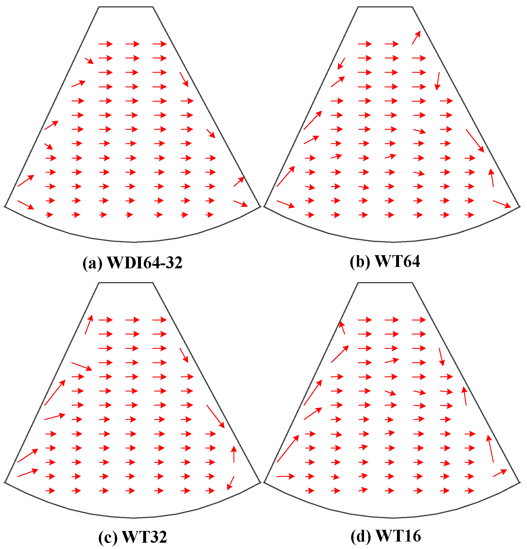
Figure 9.
Figure 9a is the vector map obtained by iterative multi-grid deformation technique with the size window interrogation from 64 × 64 to 32 × 32, referred to as WDI64-32.
Figure 9b is the vector map obtained by cross-correlation with the size of window templates 64 × 64, referred to as WT64.
Figure 9c is the vector map obtained by cross-correlation with the size of window templates 32 × 32, referred to as WT32.
Figure 9d is the vector map obtained by cross-correlation with the size of window templates 16 × 16, referred to as WT16. They are the measured results of velocity profile vectors in the same silt carrying flow and were calculated for effect comparison nearly simultaneously.
To estimate the accuracy of the measured profile velocities, firstly, a statistical value is obtained at each sampling position and taken as a true value. Secondly, the last obtained profile velocities are compared with the standard velocities, which are obtained by the ADCP method. Lastly, the velocity profile distribution of the silt carrying flow is obtained by statistical averages of each layer, referred to as averaged depth among 50 ultrasonic images and listed in
Table 2 and
Figure 10.
The statistical averages that are the depth-averaged velocities of profile flow field may be affected by the roughness of the coarse bed, and the depth-averaged profiles are valid over the entire flow depth [
38]. The velocity profile obtained by the ADCP is taken to be the standard velocities at the same position, which has been verified. From
Table 2 and
Figure 10, we concluded that the velocity profile obtained by the WT64 is smaller than the actual velocity (ADCP). The velocity profile obtained by the WDI64-32 is similar to actual velocity. The stability of the velocity profile obtained by the WT16 is poor. In contrast, the velocity profile obtained by the WT16 has the worst among them.
The reason for the above results can be analyzed and explained as follows. The test flow is laminar, and the viscosity of the fluid will give a resistance to flow, so the distribution of profile velocities has the logarithmic shape of the velocity profile. Due to the velocity gradient, the measurement error of the velocity profile can be expressed as follows:
where
is the actual velocity at depth
y,
is the averaged velocity at depth
y,
is the measured error between
and
, and
is the width of the interrogation.
The Formulas (9) and (10) are obtained according to Formulas (7) and (8), which can explain the effect of flow field. From the Formula (10),
means the average velocity
at depth
y is close to a value, which is lower than the actual velocity
. If the interrogation window size is smaller, the measurement error will also become less:
where
is the friction velocity,
is the von Karman constant value, which has a given typical value 0.41, and
B is around 5.0 for a smooth wall.
From
Figure 10 and the above analysis, the measurement precision can be increased from profile WT64 and profile WT32. The reason is that the spread of the correlation peak becomes wider if the window is larger. The dynamic range of the displacement scales aligns with the dimension of the interrogation window at the same displacement gradient. This will result in a rising tendency for the correlation peak width. As a result, a smaller interrogation window is more advantageous and can produce a higher particle image density. Consider an interrogation region of a given size: the interrogation region contains many more particle-image pairs with a small displacement than with a large displacement for the real-time measurement in a region with a strong velocity gradient. Therefore, smaller displacements are more favorable for the local mean displacement than large displacements.
The flow field vectors can be obtained by using a template-matching approach, that is, sub-images of the first are cross-correlated with the entire second image, but the accurate ratio decreases sharply when the window size decreases further from the observation of profile WT32 and profile WT16. When the window size decreases from 32 to 16 pixel-units, there are insufficient particle image pairs to estimate the displacement-correlation peak in the interrogation spot.
Additionally, good tracking performance cannot be assured when a big interrogation size is chosen by comparing profile WT64 with profile WT32. Furthermore, the PIV analysis is also time-consuming when only using a small interrogation size. Thus, it presents a trade-off between accuracy and efficiency. The iterative approach of the ultrasound PIV method is a compromise, as it is a coarse-to-fine interrogation scheme in essence. It considerably reduces the processing time whilst producing a slight reduction in measurement accuracy.
6. Discussions of Measurement Errors
The velocity profile distribution in silt carrying flow can be measured using ultrasound imaging and the iterative multi-grid deformation technique. The key to the visual measurement of the displacement or feature vector in the image is based on the correlation analysis between two interrogation windows. There are some errors in the flow velocity gradient across the window, because not all the particle images consistently appear in the first interrogation window and then in the next interrogation window. When the interrogation windows have not deformed, the displacement will be close to the actual displacement because the template matching method assumes that the particle image displacement is uniform over the interrogation. When the velocity gradient increases, the measurement error arises because the image deforming algorithm allows some particle images to be detected in an interrogation field. The image deforming algorithm can tolerate a much higher velocity gradient, which is why the measured velocity profile with the deforming algorithm is in great agreement with the standard profile. The image deforming algorithm has better performance than the template matching approach.
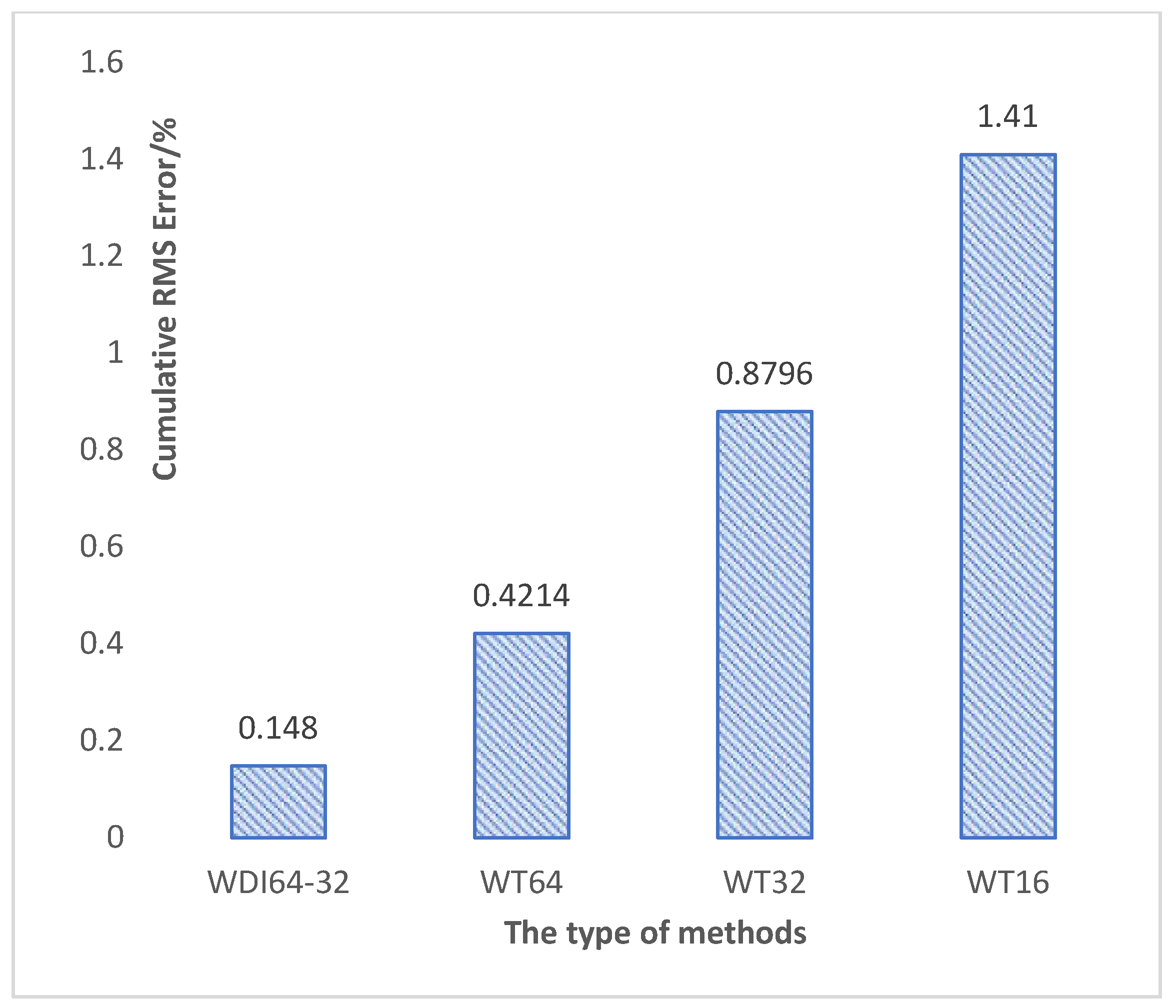
Furthermore, we take the values of the ADCP method as the reference values, and then recalculate all the RMS errors of vectors in the interrogation window of the single ultrasonic image. The cumulative RMS error is the sum of all vectors’ RMS errors in the image at a time in order to facilitate comparison. The cumulative RMS errors of the WDI64-32, WT64, WT32, and WT16 methods are shown in
Figure 11.
Figure 11 shows the cumulative RMS errors computed with the different algorithms. The mean RMS error relative to standard velocity is limited to 0.148 of the WDI64-32 algorithm, 0.4214 of the WT64 algorithm, 0.8796 of the WT32 algorithm, and it reaches 1.4148 of the WT16 algorithm. (The velocity profile value obtained by the ADCP method at eleven measurement points is taken as the standard value.)
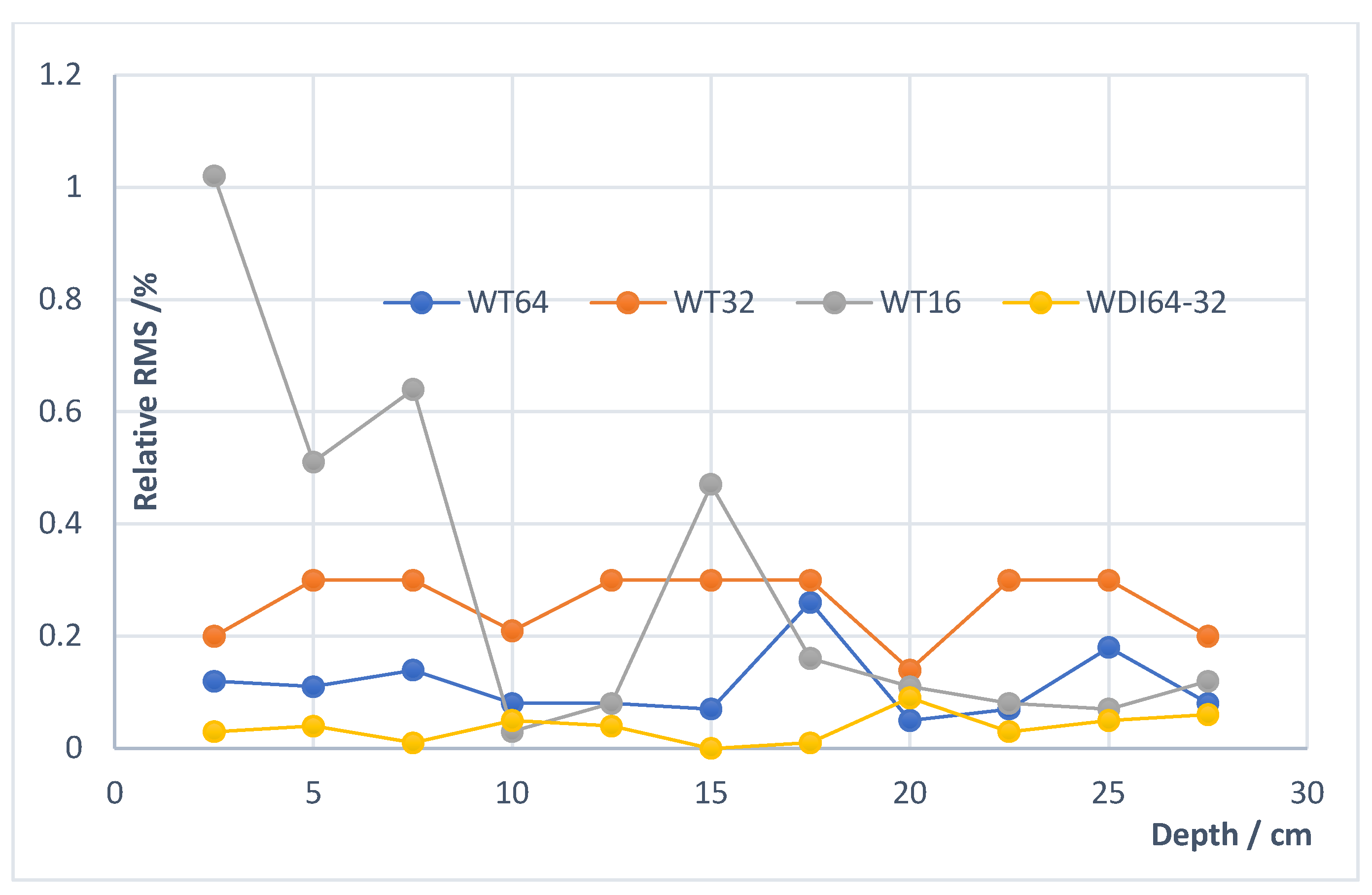
The comparisons of relative RMS errors along with the depth are shown in
Figure 12. From
Figure 12, the curve of the WDI64-32 algorithm presents the RMS errors relative to the standard value and is relatively flat. As for the curves of the WDI64-32 and WT64 algorithms, the image deformation algorithm is more suitable for the matching than the WT64 algorithm when considering the gradient. As is shown in the curves of the WT64, WT32, and WT16 methods in
Figure 12, the relative RMS error increases with the window size decrease for the measurement of the average velocity in certain conditions. When the interrogation window size decreases from 64 × 64 to 32 × 32, then up to 16 × 16 pixels, the relative RMS error is strongly influenced because the efficient particle image number decreases rapidly. To 16 × 16 pixels, there is no sufficient particle image to estimate the centroid of the correlation peak, so the RMS reaches the maximal RMS error. Therefore, the WDI64-32 algorithm gives minimal RMS error and is in excellent agreement with the reference case.
All in all, the spatial resolution increases when the window size becomes smaller from 64 to 32. However, the RMS error will increase dramatically when the window size becomes smaller from 32 to 16. The reason is that there are not enough particle images to determine the flow velocity in some positions. These results give an idea of the performance of the ultrasound PIV method compared with the conventional PIV method. The iterative multi-grid deformation algorithm has some advantages in coping with velocity gradients. The WDI64-32 algorithm shows optimal performance.
7. Conclusions
This paper describes a method for the visual measurement of velocity profile distribution in silt carrying flow using the ultrasound PIV and iterative multi-grid deformation techniques with a kind of physical model experiment. A portable medical ultrasound imaging device with a convex array probe is used to acquire the ultrasonic image in the sediment-laden flow. Conventional techniques, such as the optical PIV technique, require a clear flow condition or optical access to capture particle images. However, our ultrasound PIV method does not have this limitation. It has the advantage of simplicity and accessibility with the help of an interface software in actual applications. An ultrasound imaging measurement system can realize the visual measurement of the flow field and velocity profile distribution in silt carrying flow. The biggest advantages of this system are the portable device and the good penetrability for silt carrying flow during kinds of physical model tests.
This paper also provides an iterative multi-grid deformation method to improve the spatial resolution of ultrasonic images and the processing speed of the flow velocity measurement. A hierarchical approach is used to improve the spatial resolution through which the sampling grid is continually decreased, and the interrogation window size is also simultaneously decreased. The interrogation process is from coarse to fine. However, the decrease in interrogation window size can decrease the peak’s signal-to-noise ratio. Physical model experiments assess the performance of the PIV technique based on the ultrasonic imaging system. The velocity vectors obtained by using the WDI64-32 algorithm are the most in agreement with standard values (ADCP algorithm) compared with the WT64 algorithm, the WT32 algorithm, and the WT16 algorithm. Their RMS errors are 0.148, 0.4214, 0.8796, and 1.4148 at the certain condition, respectively. Additionally, profiles of streamwise velocity are often irregular and have a great velocity gradient. Therefore, the window deformation technique is necessary to compensate for the velocity gradient effect to optimize the accuracy of the real-time and visual measurement.


