Accurate Prediction and Key Feature Recognition of Immunoglobulin

Abstract

Immunoglobulin, which is also called an antibody, is a type of serum protein produced by B cells that can specifically bind to the corresponding antigen. Immunoglobulin is closely related to many diseases and plays a key role in medical and biological circles. Therefore, the use of effective methods to improve the accuracy of immunoglobulin classification is of great significance for disease research. In this paper, the CC–PSSM and monoTriKGap methods were selected to extract the immunoglobulin features, MRMD1.0 and MRMD2.0 were used to reduce the feature dimension, and the effect of discriminating the two–dimensional key features identified by the single dimension reduction method from the mixed two–dimensional key features was used to distinguish the immunoglobulins. The data results indicated that monoTrikGap (k = 1) can accurately predict 99.5614% of immunoglobulins under 5-fold cross–validation. In addition, CC–PSSM is the best method for identifying mixed two–dimensional key features and can distinguish 92.1053% of immunoglobulins. The above proves that the method used in this paper is reliable for predicting immunoglobulin and identifying key features.

1. Introduction

Immunoglobulin, also known as an antibody, is a serum protein present in humans. When the immune system of the body encounters invasion, B cells are stimulated, depending on the degree of invasion, to produce different numbers of globins that can specifically bind to the corresponding antigen and provide immune functions. Immunoglobulins, therefore, play a key role in protecting the human body from internal and external threats and help maintain the stability of the immune system and self–tolerance [1]. Immunoglobulins are closely related to disease treatment and have been used for a long time in the study of multiple autoimmune diseases. For example, treatment with intravenous immunoglobulin in patients with systemic sclerosis not only alleviates muscle symptoms but also ameliorates systemic inflammation in skin disease [2]. Immunoglobulins also exert a remission effect against different forms of lupus erythematosus skin disease, and, even when used in the treatment of Behcet’s disease, there is a sustained response over time without any side effects [3,4]. The in–depth study of immunoglobulins can better determine the immune mechanism and develop effective drugs to treat diseases [5].

In fact, the detection of immunoglobulins has attracted the attention of researchers. Marcatili et al. developed a strategy to predict the 3D structure of antibodies [6]. This strategy only approximately ten minutes on average to build a structural model of the antibody. This process is fully automated while achieving a very satisfactory level of accuracy. In order to identify antigen–specific human monoclonal antibodies, Liu et al. successfully developed an antibody clone screening strategy based on clone kinetics and relative frequency [7]. This method can simplify the subsequent experimental screening. The enzyme–linked immunosorbent assay showed that at least 52% of the putative positive immunoglobulin heavy chains constituted antigen–specific antibodies. In addition, Salvo et al. introduced biosensors for detecting the total content of immunoglobulins, including electrochemical biosensors, optical biosensors, and piezoelectric biosensors [8]. Immunoglobulin optical biosensors are mainly based on surface plasmon resonance detection, but the current limitation is that almost all of them only work in buffer solutions. These current state-of-the-art technologies do help the study of immunoglobulin, but biochemical experiments usually need considerable money or time [9,10].

With the proliferation of protein data, we urgently need effective and efficient computational methods to identify immunoglobulins, and the first step to reveal the function of immunoglobulins is to accurately identify them [11,12]. Over the past decade, a remarkable number of machine learning–based techniques for protein sequence analysis have been developed [13,14]. The amino acid composition is an important factor for protein identification. The amino acid composition (ACC) model, as a commonly used feature representation method, was used to represent the normalized frequency of natural amino acids in peptide chains [15,16,17,18]. Subsequently, the concept of pseudo amino acid composition (PseACC), also based on the amino acid sequence, was proposed as a widely used method [19,20,21,22,23]. An improved feature extraction method based on the amino acid composition of pseudo amino acid composition is better than the feature extraction method of amino acids in the protein prediction model because, not only the amino acid composition but also the physical and chemical properties of the correlation between two residues are included [24,25,26,27]. Inspired by the pseudo amino acid composition, a pseudo k–tuple reduced amino acid composition (PseKRAAC) model was proposed by reducing the computational barriers for complexity reduction of proteins by reducing the use of amino acid letters [28].

The above methods focus mainly on the feature representation of protein sequences. To discriminate between immunoglobulins and non immunoglobulins, Tang et al. subsequently proposed a prediction model based on a support vector machine for the combination of pseudo amino acid composition and nine physical and chemical properties of amino acids [29]. However, this model passed 105 features, and jackknife experimental results indicated that 96.3% of the immunoglobulins could be correctly predicted, a result that awaits further improvement. How key features are additionally exploited to recognize immunoglobulins remains to be investigated.

In this paper, two feature representation methods, profile–based cross covariance (CC–PSSM) [30] and monoTriKGap [31] were selected to explore the accurate prediction problems of immunoglobulins. With the application of MRMD1.0 and MRMD2.0 feature selection techniques, feature dimension screening of two–dimensional key features achieved a high identification effect. The results showed that the best feature subset generated by the monoTriKGap feature extraction method was able to correctly predict 99.6% of the immunoglobulins by the support vector machine(SVM) classifier [32] based on sequential minimal optimization. The CC–PSSM feature extraction method was better able to identify key features discriminating immunoglobulins, and the identified two–dimensional mixed key features were validated by the multilayer perceptron classifier and could correctly identify 92.1% of the immunoglobulins. In addition, the performance of different feature extraction methods under different classifiers is compared, which proves that the method in this paper is reliable for immunoglobulin research.

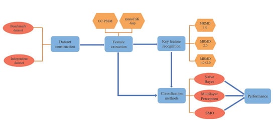
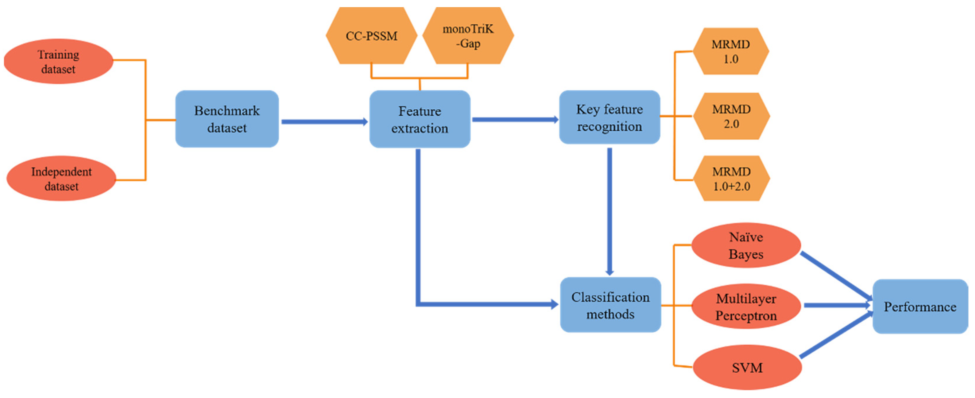
2. Materials and Methods

The main steps and processes of this paper are presented in Figure 1. The steps are summarized as follows:

• Building datasets;
• CC–PSSM and monoTriKGap were selected as feature representation methods to obtain feature sets;
• MRMD1.0 and MRMD2.0 feature selection methods were selected to acquire two–dimensional key features and two–dimensional mixed key features, respectively;
• Three classifiers, Naïve Bayes, SVM, and multilayer perceptron, were selected for k–fold cross–validation to predict immunoglobulins.

This paper shows that these three classifiers chosen in the text work better than the others through comparison. Meanwhile, the independent test set shows that the model in this paper has good generalization performance.

2.1. Dataset Construction

In this part, we will introduce the establishment of benchmark data. Since immunoglobulins are often found on or outside the cell membrane, to ensure proper discrimination, we picked a certain number of immunoglobulins both at the cell membrane and extracellularly. Immunoglobulin and non immunoglobulin sequences were downloaded from the UniProt [33] database. To establish a benchmark dataset, the following steps were taken. Protein sequences containing the nonstandard amino acid characters “B”, “J”, “O”, “X”, “U” and “Z” were first deleted. Second, to avoid overfitting caused by homologous bias and to reduce redundancy, the CD–Hit program [34,35] was selected to set a 60% sequence identity cutoff to remove highly similar sequences. Finally, if a certain protein sequence was a subsequence of other proteins, it was also removed. Considering that we needed to avoid the influence of the expression of different protein sequences on the predicted effects, we selected only human, mouse, and rat samples.

After filtering, immunoglobulin dataset samples are represented by $I^{+}$, non immunoglobulin dataset samples by $I^{-}$, and the benchmark dataset is a combination of $I^{+}$ and $I^{-}$

$$I=I^{+}\cup I^{-}$$

(1)

The $I^{+}$ dataset includes 109 positive samples, and the $I^{-}$ dataset includes 119 negative samples. Therefore, the benchmark dataset consists of 228 protein sequences, and the detailed information is shown in

Table 1. Distribution of sample sequence lengths in immunoglobulin and non immunoglobulin datasets.

Sequence Length (Amino Acids)	Immunoglobulin Dataset			Non Immunoglobulin Dataset
	Human	Mouse	Rat	Human	Mouse	Rat
<400	26	11	3	16	31	3
400–700	22	12	2	8	24	2
>700	20	10	3	5	28	2

. These can be downloaded for free from https://github.com/gongxiaodou/Immunoglobulin (accessed on 21 July 2021). To further validate the accuracy of the method in this paper for immunoglobulin prediction and the reliability of key feature identification, we used two datasets for independent testing.

2.2. Feature Extraction

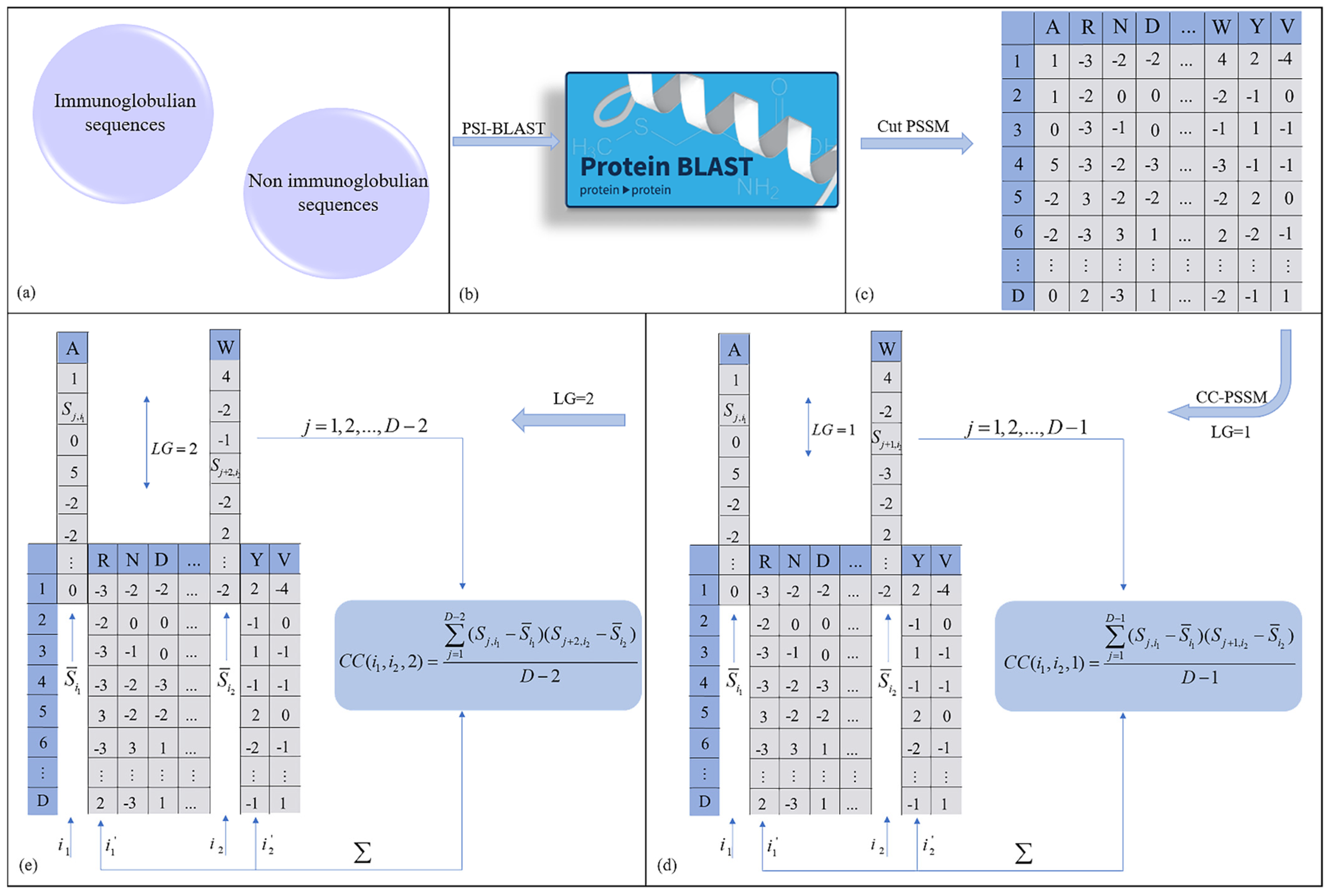
2.2.1. Profile–Based Cross Covariance (CC–PSSM)

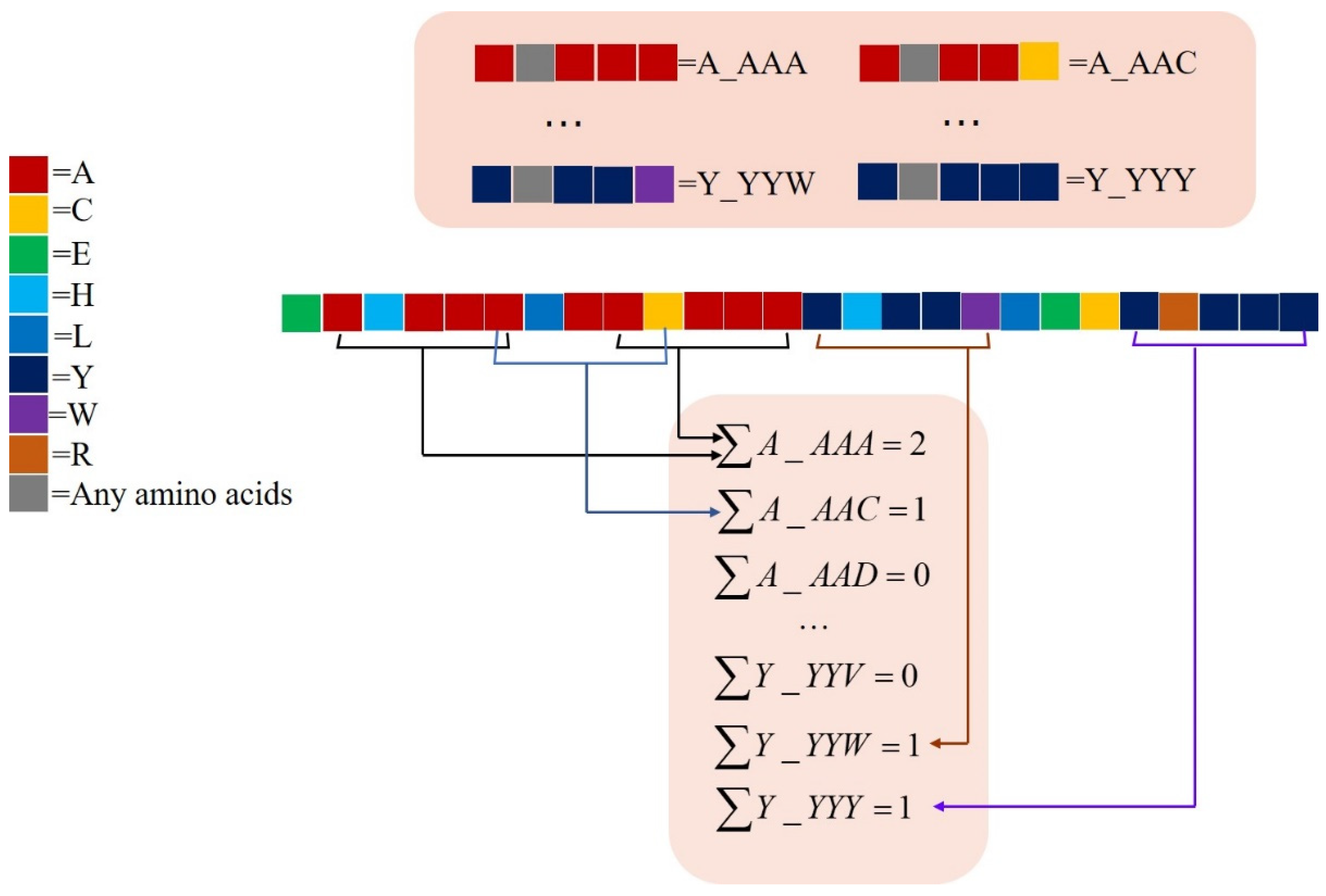
The CC–PSSM feature representation method is based on the position–specific scoring matrix (PSSM) [36,37] as a feature. Each immunoglobulin sequence runs PSI–BLAST [38] through NCBI’s NR database for local information comparison to obtain PSSM matrix information. The element $S_{ji}$ in the PSSM matrix represents the substitution score of the amino acid $i$ at the sequence position $j$. The twenty kinds of natural amino acids are composed of a set $\{A,R,N,D,C,Q,E,G,H,I,L,K,M,F,P,S,T,W,Y,V\}$.

Each protein sequence containing D residues can be represented as

$$R=R_1{R}_2{R}_3{R}_4\dots R_D$$

(2)

where $R_j(j=1,2,3\dots D)$ represents the position $j$ of the residue in the protein sequence sample $R$.

CC–PSSM [39] transforms PSSM matrices of different sizes into vectors of the same length. CC [40] was used to calculate the different properties of the two residues separated along with the sequence lag. The formula was calculated as follows

$$CC(i_1,i_2,LG)={\displaystyle \sum _{j=1}^{D-LG}(S_{j,i_1}-}{\overline{S}}_{i_1})(S_{j+LG,i_2}-{\overline{S}}_{i_2})/D-LG$$

(3)

where $i_1$ $i_2$ represents two different amino acids, ${\overline{S}}_{i_1}$, ${\overline{S}}_{i_2}$ represents the mean of substitution scores for amino acids $i_1$ and $i_2$ along the sequence, and D represents the length of the protein sequence. Calculated in this way, the PSSM matrix resulting from each protein sequence alignment will be transformed into a vector of length $380\ast lag$, and lag is the maximum value of LG (LG = 1, 2…, lag). In this study, we set the maximum lag number to 2. When LG = 1, the extracted features such as “CC(A,R,1)”, “CC(A,N,1)”, “CC(A,D,1)”, etc., are transformed into a vector of length 380. When LG = 2, the extracted features such as “CC(A,R,2)”, “CC(A,N,2)”, “CC(A,D,2)”, etc., are transformed into a 380–length vector. Therefore, each protein sample was finally computationally transformed into a vector of length 760. The demonstration process is shown in Figure 2.

2.2.2. monoTriKGap

The monoTriKGap feature extraction method was used in this article, which stems from PyFeat. This method has been widely used in the prediction of proteins and other biologies [41,42,43]. PyFeat differs from the previous adoption of Kmer [44] frequency by setting the important parameter KGap. The kmer frequency has always been a principal method for extracting the local characteristics. However, as the length of K, the subsequence continues to increase, and the number of features also increases sharply. For proteins, there is a surge quantity of features produced due to the higher number of amino acids. Thus, monoTriKGap uses KGap parameters to address this limitation [45,46]. In the monoTriKGap model, the parameter KGap can be set to 1, 2, or 3.

The important point is that, while generating the full feature set, monoTriKGap chooses the AdaBoost classification model [47] to reduce the redundant features to generate the best feature set. Utilizing this model not only reduces the feature dimensionality but also guarantees robustness under high–dimensional feature multicollinearity. In this study, to reduce data sparsity, KGap was set at 1. When KGap = 1, the characteristic shape is $X\_XXX$, where X is the twenty natural amino acids, denoted as

$$\mathrm{X}=\left\{\mathrm{A},\mathrm{C},\mathrm{D},\mathrm{E},\mathrm{F},\mathrm{G},\mathrm{H},\mathrm{I},\mathrm{K},\mathrm{L},\mathrm{M},\mathrm{N},\mathrm{P},\mathrm{Q},\mathrm{R},\mathrm{S},\mathrm{T},\mathrm{V},\mathrm{W},\mathrm{Y}\right\}$$

(4)

Features such as “A_AAA”, “A_AAC”, etc., are generated. The full dataset generated by the monoTriKGap model at this time had 160,000 features and was automatically optimized by AdaBoost to generate the best feature set containing 212 more discriminative features. When KGap = 1, taking the sequence “EAHAAALAACAAAYHYYWLECYRYYY” as an example, the feature dataset generation is demonstrated in Figure 3.

2.3. Classifier

To further accurately predict whether the protein sequence is an immunoglobulin, this classification problem is regarded as a dichotomy problem [48,49]. Three classifiers were employed in this paper to select those that could predict immunoglobulins more accurately by comparison. The three classifiers used were Naïve Bayes, SVM, and multilayer perceptron.

Naïve Bayes (NB) [50,51], as a Bayesian probabilistic classifier, is assumed to be independent and equal across features for classification. The independence of samples from each other is not affected by either and does not cause interference with the classification results. Based on this characteristic, the feature classification of samples avoids the linear influence, so that it is also easy to implement, has fast running speed, and is noise insensitive in high–dimensional features, which is beneficial for applications. As a supervised machine learning method, the support vector machine can solve both classification and regression problems. This paper is a binary classification problem, the basic idea of which is to separate samples of different categories by finding a separation hyperplane. In order to reduce the amount of computation and memory, John C. Platt proposed sequential minimal optimization [52,53] based on support vector machines (SVMs) [54,55,56]. This is widely used because it decomposes the large quadratic programming (QP) problem that SVMs need to solve into a series of minimum possible QP problems, avoiding time–consuming iterative optimization of in–house QPs. The choice of kernel function for support vector machines is very important. On the same dataset, different kernel function algorithms may have different prediction effects. In general, appropriate kernel functions can improve the prediction accuracy of the model, such as linear kernel function, polynomial kernel function, and radial basis function (RBF). The multilayer perceptron (MLP) [57] is a simple artificial neural network, in which neurons are connected between adjacent layers and there is no connection between neurons in each layer. It maps the input dataset to the output set in a feedforward manner, and the output of each node is a weighted unit followed by a nonlinear activation function to distinguish nonlinearly separable data. The multilayer perceptron is usually trained using backpropagation. Previously, the MLP results for solving classification problems have been well verified.

2.4. Key Feature Recognition

In the feature extraction subsection, several hundred features were extracted by CC–PSSM and monoTriKGap methods. However, there was redundancy between these features. This section introduces the identification of two–dimensional key features by means of MRMD1.0 and MRMD2.0 feature selection techniques, reaching the experimental effect of predicting immunoglobulins with fewer characteristics.

The feature selection method of MRMD1.0 [58,59] is decided in two main parts: one is the correlation between the characteristic and the instance class standard, and the Pearson correlation coefficient is used to calculate the correlation between the characteristic and the class standard. The other part is the redundancy among characteristics. This method makes use of three distance functions: Euclidean distance, cosine distance, and the Tanimoto coefficient, to calculate the complexity among characteristics. A larger Pearson correlation coefficient indicates that the features are more closely related to the class scale, and a larger distance indicates less redundancy among the characteristics. Finally, MRMD1.0 generates feature subset ranking information with strong correlation to class labels and low redundancy between features. Here, we selected the first two features as the two–dimensional key features identified by MRMD1.0 based on the ranking information.

MRMD2.0 [60], as a currently commonly used feature ranking and dimension reduction tool, contains seven means of feature ranking: MRMR, LASSO, ANOVA, and MRMD [61]. MRMD2.0 utilizes the PageRank algorithm technique to calculate a directed graph score for each feature, ranking features according to score. Meanwhile, users can also custom–select feature numbers, yielding the optimal feature subset with maximum relevance and minimum redundancy balanced. Here, we chose to screen 2 optimal features as the key features for immunoglobulin recognition.

2.5. Performance Evaluation

To further estimate the classification performance of our selected feature set and two–dimensional key features, the TP rate (TPR), FP rate (FPR) [62], precision [63,64,65,66], Matthews correlation coefficient (MCC) [67], and accuracy (ACC) [68,69,70,71] were calculated and compared to obtain the best immunoglobulin accurate prediction and key feature identification method. Individual performance metrics were calculated as follows

$$\{\begin{array}{l}TPR=\frac{TP}{TP+FN}\\ FPR=\frac{FP}{FP+TN}\\ precision=\frac{TP}{TP+FP}\\ MCC=\frac{TP\ast TN-FP\ast FN}{\sqrt{(TP+FP)(TP+FN)(TN+FP)(TN+FN)}}\\ ACC=\frac{TP+TN}{TP+FP+TN+FN}\end{array}$$

(5)

TP indicates the amount of exactly forecasted immunoglobulin samples, and FN indicates the amount of exactly forecasted non immunoglobulin samples [72]. TPR represents the ratio of correctly forecasted immunoglobulins, and FPR represents the ratio of inexactly forecasted non immunoglobulins. Precision indicates the rate of correctly classifying positive datasets. MCC indicates the correlation between the actual and forecasted classification. ACC indicates the ratio of exactly classified datasets.

3. Results and Discussion

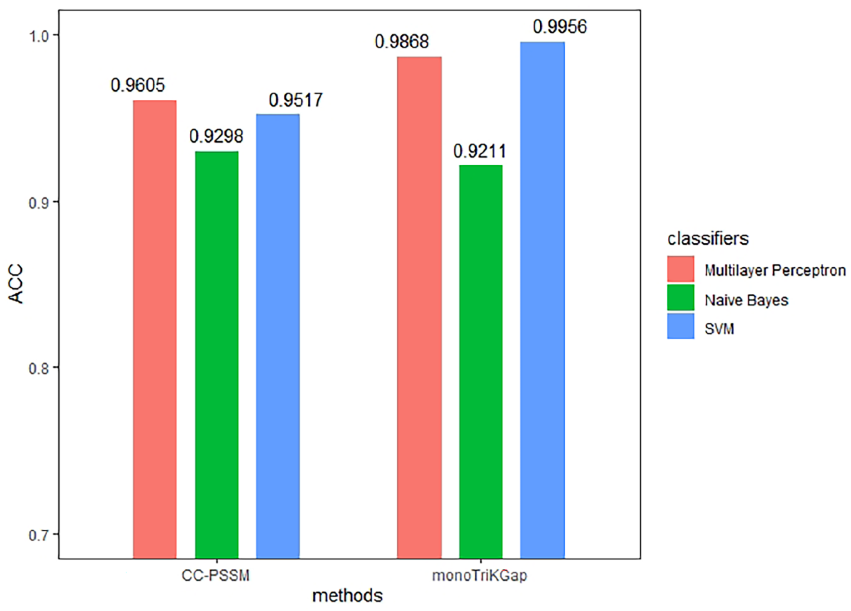
3.1. Comparison of Different Feature Extraction and Classification Methods

According to the previous article, this study compared the prediction effects of the three classifiers: Naïve Bayes, SVM, and multilayer perceptron. Among them, the parameters of the three classifiers adopted the default parameters built in the algorithm. The default kernel function of SVM was linear kernel function, and the value of penalty coefficient was C = 1.0. The topology of the multilayer perceptron was selected as a simple 3–layer network, including an input layer, a hidden layer, and an output layer, using the Sigmoid function as the activation function. CC–PSSM and monoTrikGap feature extraction methods were compared with previous research results, and we tested the accuracy of the classification of the immunoglobulin dataset through 5–fold cross validation [73]. The predictions obtained from the 760 features extracted by the CC–PSSM method, and the 212 best feature subsets generated by the monoTriKGap method with the three different classifiers mentioned above, are presented in

Table 2. Compare the results of different feature methods under different classifiers.

Method	Classifier	TPR	FPR	Precision	MCC	auROC	ACC
CC–PSSM	NB	0.930	0.072	0.930	0.860	0.951	0.9298
	MLP	0.961	0.041	0.961	0.921	0.994	0.9605
	SVM	0.952	0.050	0.952	0.904	0.951	0.9517
monoTriKGap	NB	0.921	0.081	0.921	0.842	0.951	0.9211
	MLP	0.987	0.013	0.987	0.974	0.997	0.9868
	SVM	0.996	0.004	0.996	0.991	0.996	0.9956
Tang et al. [29]	SVM	0.963	0.025	\	\	0.994	0.9690

, and the contrasts of ACC values are presented in Figure 4.

The data in Table 2 show that for the CC–PSSM feature extraction method, the ACC values of the multilayer perceptron classifier are higher than those of Naïve Bayes and SVM. Using multilayer perceptron to predict the immunoglobulin TPR value, the value reached 0.961, the FPR value reached 0.041, the MCC value reached 0.921, and the ACC value reached 96.0526%. The ROC curve area was 0.994. Compared with the Naïve Bayes classifier, the ACC value increased by 3.1%. For the monoTriKGap feature extraction method, the TPR, precision, ACC, and other values of the SVM classifier were higher than the values of Naïve Bayes and multilayer perceptron. Using SVM to predict the immunoglobulin TPR value reached 0.996, the FPR value reached 0.004, the MCC value reached 0.991, and the ACC value reached 99.5614%. The ROC curve area was 0.996. Compared with the Naïve Bayes classifier, the ACC value increased by 7.5%.

Through comparison and analysis, the study found that the SVM classification result of the best feature subset extracted by monoTriKGap improved compared with the multilayer perceptron classification result of the feature subset extracted by CC–PSSM and the prediction model proposed by Tang et al. [29]. This shows that employing the monoTriKGap feature extraction method to generate the best feature subset and SVM can achieve a higher prediction effect, which is most conducive to the accurate prediction of immunoglobulins.

Then, we compared the performance of SVM under three kinds of kernel functions (linear kernel function, quadratic polynomial kernel function, and radial basis kernel function), as shown in

Table 3. The prediction results of the best feature subset of monoTriKGap under different kernel functions of support vector machine.

Kernel Function	TPR	FPR	Precision	MCC	auROC	ACC
liner kernel	0.996	0.004	0.996	0.991	0.996	0.9956
polynomial kernel	0.864	0.138	0.864	0.728	0.863	0.8640
RBF	0.746	0.277	0.821	0.554	0.734	0.7456

.

It can be seen from Table 3 that when using the best feature subset of monoTriKGap, the prediction effect of the linear kernel function was better than the other two kernel functions. The linear kernel function used to predict the accuracy of immunoglobulin reached 99.56%, the MCC value reached 0.991, and the precision value reached 0.996. The ACC value was 13.16% higher than the polynomial kernel function and 25% higher than the radial basis kernel function. Therefore, this paper adopted the linear kernel function as the kernel function of the support vector machine.

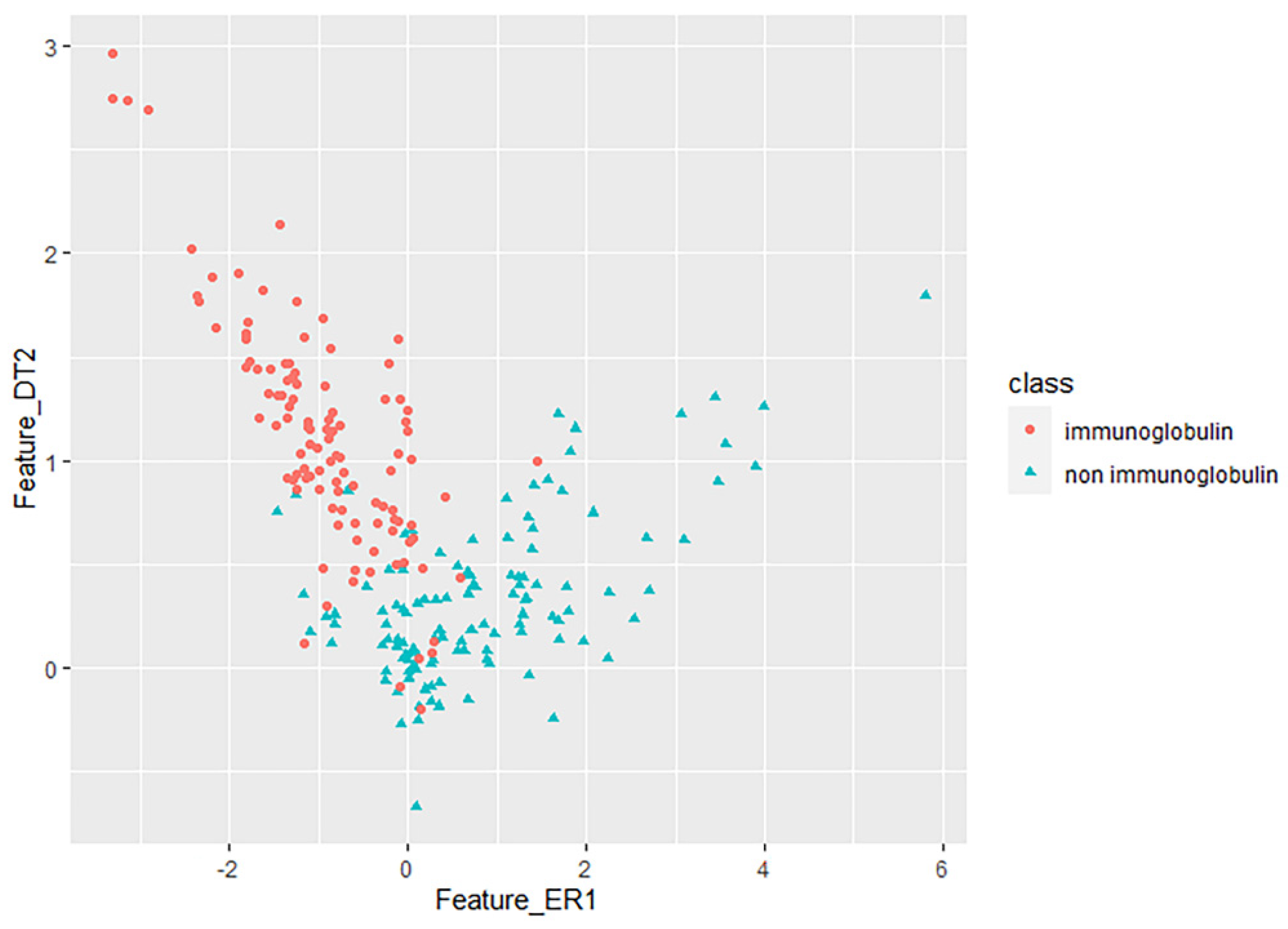
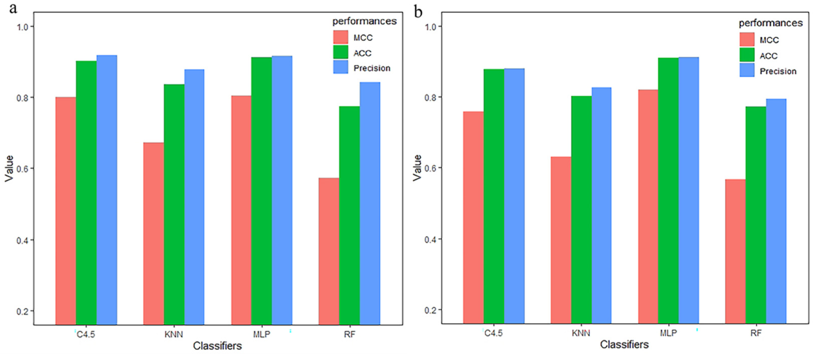
3.2. Key Feature Analysis

This study introduced the use of MRMD1.0 and MRMD2.0 for two–dimensional key feature recognition. Key feature recognition and analysis were performed on the feature subsets extracted based on CC–PSSM and monoTriKGap, respectively.

First, based on the 760 features extracted by CC–PSSM, MRMD1.0 was used to reduce the dimensionality, and the first two features were selected according to the ranking information to be CC(P, D, 2) and CC(E, R, 1) as the first group two–dimensional key features. Second, MRMD2.0 was used to reduce the dimensionality of the original feature set; the number of generated features was set to two, and the two matched features were CC(D, T, 2) and CC(H, C, 1) as the second group of two–dimensional key features. Then, the key features of the first two groups were combined in any two pairs to generate four sets of 2–dimensional feature combinations that were different from the first two groups. The feature combined with the largest classification index ACC value, namely CC(E, R, 1) and CC(D, T, 2), were selected as the two–dimensional key features of MRMD1.0 and MRMD2.0.

Based on the 212 best features extracted by monoTriKGap, the above steps were also performed. The first two–dimensional key features, including D_DDD and H_HHD, were obtained through MRMD1.0. Through MRMD2.0, the second set of two–dimensional key features, including F_HHV and D_HHF, were obtained. By comparing the ACC values of four sets of two–dimensional hybrid features in any combination, we obtained the hybrid two–dimensional key features of MRMD1.0 and MRMD2.0, including H_HHD and F_HHV.

To analyse the ability of each group of key features to distinguish immunoglobulins, the classification performance of the three groups of key features of CC–PSSM and monoTriKGap was evaluated. Three classifiers of Naïve Bayes, SVM, and multilayer perceptron classifiers were used under 5–fold cross validation. The results of the two–dimensional key feature analysis are shown in

Table 4. Classification results of different two–dimensional key feature recognition methods.

Method	Selection	Classifier	TPR	FPR	Precision	MCC	auROC	ACC
	MRMD1.0	NB	0.890	0.113	0.892	0.781	0.950	0.8904
		MLP	0.904	0.101	0.908	0.810	0.946	0.9035
		SVM	0.868	0.139	0.877	0.744	0.865	0.8684
CC–PSSM	MRMD2.0	NB	0.846	0.158	0.849	0.694	0.875	0.8465
		MLP	0.825	0.177	0.825	0.648	0.877	0.8246
		SVM	0.803	0.202	0.804	0.605	0.801	0.8026
	MRMD 1.0+2.0	NB	0.886	0.121	0.895	0.780	0.955	0.8859
		MLP	0.921	0.081	0.921	0.842	0.934	0.9211
		SVM	0.895	0.112	0.902	0.796	0.891	0.8947
	MRMD1.0	NB	0.535	0.439	0.576	0.119	0.563	0.5351
		MLP	0.526	0.461	0.537	0.068	0.505	0.5263
		SVM	0.531	0.509	0.562	0.052	0.511	0.5307
MonoTriKGap	MRMD2.0	NB	0.491	0.500	0.496	–0.009	0.514	0.4804
		MLP	0.491	0.499	0.497	–0.008	0.501	0.4912
		SVM	0.522	0.522	0.522	0.000	0.500	0.5219
	MRMD 1.0+2.0	NB	0.539	0.442	0.561	0.108	0.572	0.5395
		MLP	0.522	0.454	0.550	0.081	0.514	0.5219
		SVM	0.522	0.522	0.522	0.000	0.500	0.5219

.

The research results in Table 4 show that after the features extracted by CC–PSSM reduce the dimensionality, the mixed two–dimensional key features of MRMD1.0 and MRMD2.0 have better classification performance than the single–obtained two–dimensional key features. The ACC value of mixed two–dimensional key features using the multilayer perceptron classifier was 92.1053% higher than the ACC value of the single group of two–dimensional key features, which were 90.3509% and 84.6491%, respectively. At this time, the TPR was 0.921, the FPR was 0.081, the MCC was 0.842, and the ROC curve area was 0.934. Similarly, after the features extracted by monoTriKGap reduced the dimensionality, the classification performance of the mixed two–dimensional key features was also better than the classification performance of a single group of two–dimensional key features. At this time, MRMD1.0 and MRMD2.0 mixed two–dimensional key features using a Naïve Bayes classifier to achieve the ACC value of 53.9474%. Most importantly, the mixed two–dimensional key features of the CC–PSSM feature extraction method were better than monoTriKGap, which proves that the CC–PSSM feature extraction method could better identify the key features to distinguish immunoglobulins. Figure 5 shows the scatter plot of the 2–dimensional mixed features recognized by CC–PSSM to distinguish immunoglobulins from non immunoglobulins.

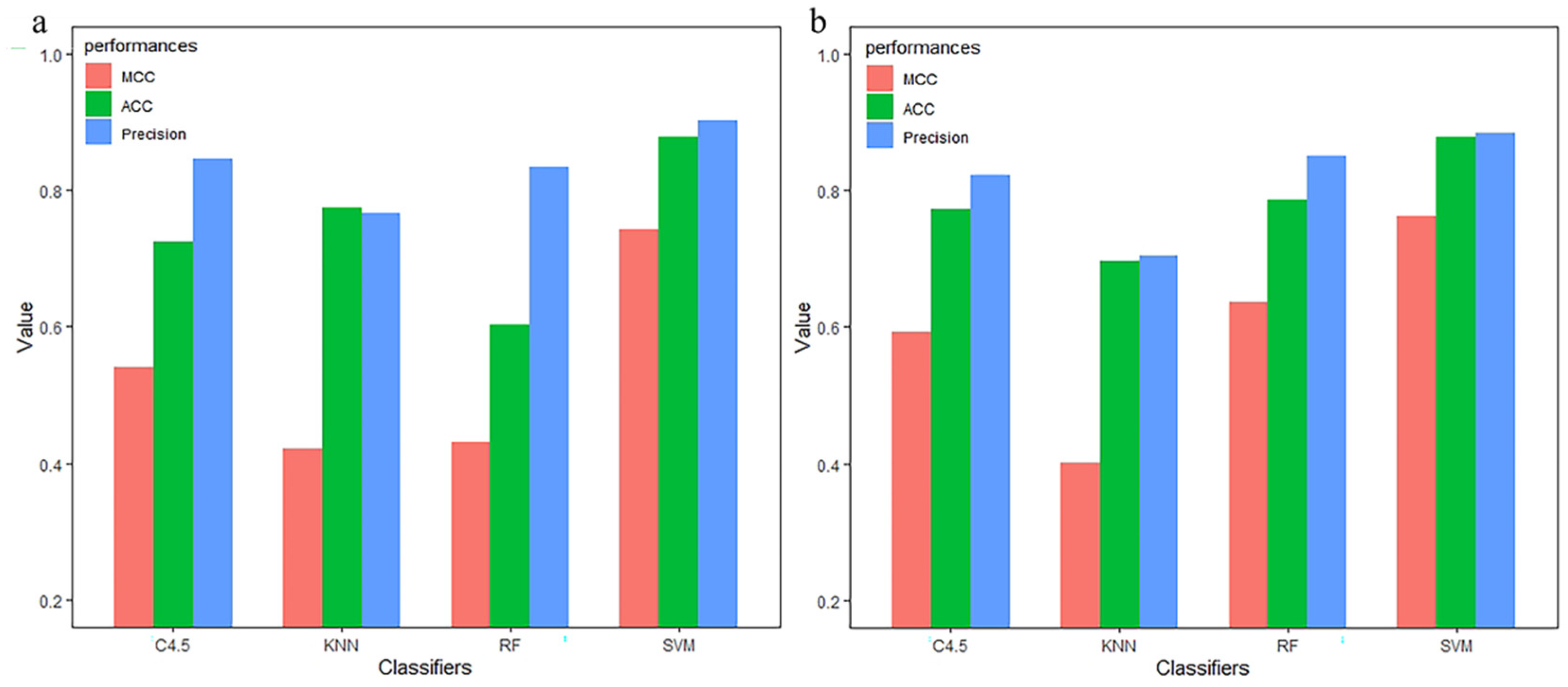
3.3. Compared with Other Classifiers

For a fair comparison, we further studied the performance of the other three classifiers on the same benchmark dataset, namely k–Nearest Neighbor (KNN) [74], C4.5 [75], and random forest (RF) [76,77]. The parameters of the classifier were set to default values. The basic idea of KNN is that there are always k most similar samples in the feature space. If most of the samples belong to a certain category, the sample also belongs to this category. Here, we set the value of k in our model to be 3. The C4.5 algorithm, as a classification decision tree algorithm [78] that uses the information gain rate to select node attributes, is pruned in the tree construction and the generated classification rules are easy to understand. Here we set the default confidence factor for pruning c = 0.25.

The previous study showed that monoTriKGap had a better predictive ability for immunoglobulin under the SVM classifier. Next, we used the best 212 feature subsets extracted by monoTriKGap for performance evaluation under KNN, C4.5, and RF. The comparison results are recorded in

Table 5. Comparison of features extracted by monoTriKGap under other classifiers.

Method	Classifier	TPR	FPR	Precision	MCC	auROC	ACC
monoTriKGap	SVM	0.996	0.004	0.996	0.991	0.996	0.9956
	KNN	0.732	0.288	0.787	0.510	0.831	0.7325
	C4.5	0.833	0.169	0.833	0.666	0.838	0.8333
	RF	0.969	0.034	0.971	0.940	0.988	0.9693

. The data in Table 5 further verifies that the monoTrikGap feature extraction method generated the best feature subset using the SVM classifier, had a high predictive effect, and could accurately distinguish between non immunoglobulins and immunoglobulins.

For the recognition of key features, through the previous research, we obtained that the mixed two–dimensional key features of the CC–PSSM feature extraction method had better recognition capabilities by the multilayer perceptron classifier. Next, the mixed two–dimensional key features of CC(E, R, 1) and CC(D, T, 2) were used to explore the classification performance under KNN, C4.5, and RF. The comparison results are recorded in

Table 6. MRMD1.0+MRMD2.0 recognizes the comparison of the two–dimensional key features represented by CC–PSSM under other classifiers.

Method	Selection	Classifier	TPR	FPR	Precision	MCC	auROC	ACC
CC–PSSM	MRMD 1.0 + 2.0	MLP	0.921	0.081	0.921	0.842	0.934	0.9211
		KNN	0.895	0.106	0.895	0.789	0.928	0.8947
		C4.5	0.904	0.098	0.904	0.807	0.897	0.9035
		RF	0.886	0.114	0.886	0.771	0.930	0.8859

. The data in Table 6 shows that the original classifier we used does have better performance than other methods.

3.4. Independent Test Set Evaluation

In order to evaluate the generalization ability of monoTriKGap and CC–PSSM models, we conducted two independent tests. Each test set had two tasks: one was to evaluate the generalization ability of monoTriKGap optimal feature subset for accurate prediction of immunoglobulin under SVM, and the other was to evaluate the generalization ability of CC–PSSM for recognition of key features of immunoglobulin under MLP.

In the first group, 112 sequences from human and rat data were selected as the training set, and 116 sequences from mouse data were selected as the test set, including 33 immunoglobulins and 83 non immunoglobulins. The second group selected 112 human and rat sequences in the benchmark dataset as the training set. Thirty–three immunoglobulin sequences and thirty–three non immunoglobulin sequences from mouse were selected to form a test set. Details are shown in

Table 7. Details for each group of independent test sets.

	Training Dataset			Independent Dataset
	Composition	Positive	Negative	Composition	Positive	Negative
Group1	human, rat	76	36	mouse	33	83
Group2	human, rat	76	36	mouse	33	33

.

The 212 optimal feature subsets generated by each group of monoTriKGap were trained under different classifiers, and the ACC value comparison of the test set is shown in Figure 6. Figure 6a shows that the first set accurately predicted 87.93% of immunoglobulins under SVM, which is higher than the accurate values of C4.5, KNN, and RF (72.14%, 77.58%, and 60.34%, respectively). Figure 6b shows that the second test set accurately predicted 87.88% of immunoglobulins under SVM, and the accuracy values higher than C4.5, KNN and RF were 77.27%, 69.69%, and 78.78%, respectively. Therefore, the two sets of data show that monoTriKGap does have a good generalization ability for the accurate prediction of immunoglobulin.

In addition, 760 features extracted by each group of CC–PSSM were reduced in dimension by MRMD1.0 and MRMD2.0, and the identified mixed two–dimensional key features CC(E, R, 1) and CC(D, T, 2) were trained. The ACC values of the test set were compared and are shown in Figure 7. Figure 7a shows that in the first test set, the multilayer perceptron classifier correctly predicted 91.07% immunoglobulin, which is 0.9% higher than the C4.5 algorithm, 7.45% higher than the KNN algorithm, and 13.49% higher than the RF algorithm. Figure 7b shows that in the second test set, the multilayer perceptron classifier correctly predicted 90.90% of immunoglobulins, which is 3.03% higher than the C4.5 algorithm, 10.6% higher than the KNN algorithm, and 13.36% higher than the RF algorithm. Combined with the two groups of data, it can be concluded that CC–PSSM has a good generalization ability for key feature recognition. However, in order to ensure the prediction and recognition ability of the model for immunoglobulins, our future work will extend the data for further study.

4. Conclusions

The main work of protein prediction consists of two steps: one step is the selection of the feature representation method, and the other step is to reduce the feature dimension and identify key features. As a significant component of the immune system, immunoglobulin is closely related to various diseases. Accurate prediction of immunoglobulin can be more beneficial to drug development and disease treatment. This research focuses on the accurate prediction of immunoglobulin and the recognition of key features. By comparing the feature representation methods of CC–PSSM and monoTriKGap, the best feature set generated by monoTriKGap through the AdaBoost classification model is found to be able to accurately predict 99.5614% of immunoglobulins under the SVM classifier. For the identification of key features, unlike the past, we considered MRMD1.0 and MRMD2.0 for key feature screening and consider two–dimensional hybrid key features. The results show that the features extracted by CC–PSSM are identified by the mixed two–dimensional key, and 92.1053% of immunoglobulins can be distinguished under the multilayer perceptron classifier. Therefore, the method used in this article can be used as a powerful means to study immunoglobulin. In future work, we will collect and expand the dataset, and use more data to verify the effectiveness of the model. In order to improve the performance of the SVM algorithm, some important parameters of the algorithm (such as penalty coefficient C) will be optimized. At the same time, to avoid overfitting, we will consider adding related regularization tests in our future work.

References

1. Almaghlouth, I.; Johnson, S.R.; Pullenayegum, E.; Gladman, D.; Urowitz, M. Immunoglobulin levels in systemic lupus erythematosus: A narrative review. Lupus 2021, 30, 867–875. [Google Scholar] [CrossRef]
2. Gomes, J.P.; Santos, L.; Shoenfeld, Y. Intravenous immunoglobulin (IVIG) in the vanguard therapy of Systemic Sclerosis. Clin. Immunol. 2019, 199, 25–28. [Google Scholar] [CrossRef] [PubMed]
3. Cantarini, L.; Stromillo, M.L.; Vitale, A.; Lopalco, G.; Emmi, G.; Silvestri, E.; Federico, A.; Galeazzi, M.; Iannone, F.; De Stefano, N. Efficacy and Safety of Intravenous Immunoglobulin Treatment in Refractory Behcet’s Disease with Different Organ Involvement: A Case Series. Isr. Med. Assoc. J. 2016, 18, 238–242. [Google Scholar] [PubMed]
4. Tenti, S.; Fabbroni, M.; Mancini, V.; Russo, F.; Galeazzi, M.; Fioravanti, A. Intravenous Immunoglobulins as a new opportunity to treat discoid lupus erythematosus: A case report and review of the literature. Autoimmun. Rev. 2018, 17, 791–795. [Google Scholar] [CrossRef] [PubMed]
5. Yu, L.; Wang, M.; Yang, Y.; Xu, F.; Zhang, X.; Xie, F.; Gao, L.; Li, X. Predicting therapeutic drugs for hepatocellular carcinoma based on tissue–specific pathways. PLoS Comput. Biol. 2021, 17, e1008696. [Google Scholar] [CrossRef] [PubMed]
6. Marcatili, P.; Olimpieri, P.P.; Chailyan, A.; Tramontano, A. Antibody structural modeling with prediction of immunoglobulin structure (PIGS). Nat. Protoc. 2014, 9, 2771–2783. [Google Scholar] [CrossRef] [PubMed]
7. Liu, J.; Li, R.; Liu, K.; Li, L.; Zai, X.; Chi, X.; Fu, L.; Xu, J.; Chen, W. Identification of antigen–specific human monoclonal antibodies using high–throughput sequencing of the antibody repertoire. Biochem. Biophys. Res. Commun. 2016, 473, 23–28. [Google Scholar] [CrossRef]
8. Salvo, P.; Vivaldi, F.M.; Bonini, A.; Biagini, D.; Bellagambi, F.G.; Miliani, F.M.; Francesco, F.D.; Lomonaco, T. Biosensors for Detecting Lymphocytes and Immunoglobulins. Biosensors 2020, 10, 155. [Google Scholar] [CrossRef]
9. Zeng, X.; Zhu, S.; Liu, X.; Zhou, Y.; Nussinov, R.; Cheng, F. deepDR: A network–based deep learning approach to in silico drug repositioning. Bioinformatics 2019, 35, 5191–5198. [Google Scholar] [CrossRef] [PubMed]
10. Ding, Y.; Tang, J.; Guo, F. Identification of drug–side effect association via multiple information integration with centered kernel alignment. Neurocomputing 2019, 325, 211–224. [Google Scholar] [CrossRef]
11. Yu, L.; Zhou, D.; Gao, L.; Zha, Y. Prediction of drug response in multilayer networks based on fusion of multiomics data. Methods 2020. [Google Scholar] [CrossRef]
12. Wei, L.; Zhou, C.; Chen, H.; Song, J.; Su, R. ACPred–FL: A sequence–based predictor using effective feature representation to improve the prediction of anti–cancer peptides. Bioinformatics 2018, 34, 4007–4016. [Google Scholar] [CrossRef]
13. Zhu, X.J.; Feng, C.Q.; Lai, H.Y.; Chen, W.; Lin, H. Predicting protein structural classes for low–similarity sequences by evaluating different features. Knowl. Based Syst. 2019, 163, 787–793. [Google Scholar] [CrossRef]
14. Tang, H.; Zhao, Y.W.; Zou, P.; Zhang, C.M.; Chen, R.; Huang, P.; Lin, H. HBPred: A tool to identify growth hormone–binding proteins. Int. J. Biol. Sci. 2018, 14, 957–964. [Google Scholar] [CrossRef]
15. Chen, W.; Feng, P.M.; Lin, H.; Chou, K.C. iRSpot–PseDNC: Identify recombination spots with pseudo dinucleotide composition. Nucleic Acids Res. 2013, 41, e68. [Google Scholar] [CrossRef] [Green Version]
16. Fu, X.; Cai, L.; Zeng, X.; Zou, Q. StackCPPred: A stacking and pairwise energy content–based prediction of cell–penetrating peptides and their uptake efficiency. Bioinformatics 2020, 36, 3028–3034. [Google Scholar] [CrossRef] [PubMed]
17. Liu, B.; Gao, X.; Zhang, H. BioSeq–Analysis2.0: An updated platform for analyzing DNA, RNA and protein sequences at sequence level and residue level based on machine learning approaches. Nucleic Acids Res. 2019, 47, e127. [Google Scholar] [CrossRef]
18. Zhai, Y.; Chen, Y.; Teng, Z.; Zhao, Y. Identifying Antioxidant Proteins by Using Amino Acid Composition and Protein–Protein Interactions. Front. Cell Dev. Biol. 2020, 8, 591487. [Google Scholar] [CrossRef]
19. Chou, K.C. Prediction of protein cellular attributes using pseudo–amino acid composition. Proteins 2001, 43, 246–255. [Google Scholar] [CrossRef] [PubMed]
20. Cai, L.; Wang, L.; Fu, X.; Xia, C.; Zeng, X.; Zou, Q. ITP–Pred: An interpretable method for predicting, therapeutic peptides with fused features low–dimension representation. Brief. Bioinform. 2020. [Google Scholar] [CrossRef]
21. Tang, Y.-J.; Pang, Y.-H.; Liu, B. IDP–Seq2Seq: Identification of Intrinsically Disordered Regions based on Sequence to Sequence Learning. Bioinformaitcs 2020, 36, 5177–5186. [Google Scholar] [CrossRef] [PubMed]
22. Tan, J.X.; Li, S.H.; Zhang, Z.M.; Chen, C.X.; Chen, W.; Tang, H.; Lin, H. Identification of hormone binding proteins based on machine learning methods. Math. Biosci. Eng. 2019, 16, 2466–2480. [Google Scholar] [CrossRef]
23. Shen, Y.; Tang, J.; Guo, F. Identification of protein subcellular localization via integrating evolutionary and physicochemical information into Chou’s general PseAAC. J. Theor. Biol. 2019, 462, 230–239. [Google Scholar] [CrossRef] [PubMed]
24. Chou, K.C.; Wu, Z.C.; Xiao, X. iLoc–Hum: Using the accumulation–label scale to predict subcellular locations of human proteins with both single and multiple sites. Mol. Biosyst. 2012, 8, 629–641. [Google Scholar] [CrossRef] [PubMed]
25. Liu, B.; Li, K.; Huang, D.S.; Chou, K.C. iEnhancer–EL: Identifying enhancers and their strength with ensemble learning approach. Bioinformatics 2018, 34, 3835–3842. [Google Scholar] [CrossRef] [PubMed]
26. Shao, J.; Liu, B. ProtFold–DFG: Protein fold recognition by combining Directed Fusion Graph and PageRank algorithm. Brief. Bioinform. 2021, 22. [Google Scholar] [CrossRef] [PubMed]
27. Zhang, D.; Chen, H.-D.; Zulfiqar, H.; Yuan, S.-S.; Huang, Q.-L.; Zhang, Z.-Y.; Deng, K.-J. iBLP: An XGBoost–Based Predictor for Identifying Bioluminescent Proteins. Comput. Math. Methods Med. 2021, 2021, 6664362. [Google Scholar] [CrossRef] [PubMed]
28. Zuo, Y.; Li, Y.; Chen, Y.; Li, G.; Yan, Z.; Yang, L. PseKRAAC: A flexible web server for generating pseudo K–tuple reduced amino acids composition. Bioinformatics 2017, 33, 122–124. [Google Scholar] [CrossRef] [Green Version]
29. Tang, H.; Chen, W.; Lin, H. Identification of immunoglobulins using Chou’s pseudo amino acid composition with feature selection technique. Mol. Biosyst. 2016, 12, 1269–1275. [Google Scholar] [CrossRef]
30. Dong, Q.; Zhou, S.; Guan, J. A new taxonomy–based protein fold recognition approach based on autocross–covariance transformation. Bioinformatics 2009, 25, 2655–2662. [Google Scholar] [CrossRef] [Green Version]
31. Muhammod, R.; Ahmed, S.; Md Farid, D.; Shatabda, S.; Sharma, A.; Dehzangi, A. PyFeat: A Python–based effective feature generation tool for DNA, RNA and protein sequences. Bioinformatics 2019, 35, 3831–3833. [Google Scholar] [CrossRef] [Green Version]
32. Ding, Y.; Tang, J.; Guo, F. Identification of drug–target interactions via multiple information integration. Inf. Sci. 2017, 418, 546–560. [Google Scholar] [CrossRef]
33. Boutet, E.; Lieberherr, D.; Tognolli, M.; Schneider, M.; Bansal, P.; Bridge, A.J.; Poux, S.; Bougueleret, L.; Xenarios, I. UniProtKB/Swiss–Prot, the Manually Annotated Section of the UniProt KnowledgeBase: How to Use the Entry View. Methods Mol. Biol. 2016, 1374, 23–54. [Google Scholar] [CrossRef] [PubMed]
34. Fu, L.; Niu, B.; Zhu, Z.; Wu, S.; Li, W. CD–HIT: Accelerated for clustering the next–generation sequencing data. Bioinformatics 2012, 28, 3150–3152. [Google Scholar] [CrossRef] [PubMed]
35. Liu, M.L.; Su, W.; Wang, J.S.; Yang, Y.H.; Yang, H.; Lin, H. Predicting Preference of Transcription Factors for Methylated DNA Using Sequence Information. Mol. Ther. Nucleic Acids 2020, 22, 1043–1050. [Google Scholar] [CrossRef] [PubMed]
36. Wang, H.; Ding, Y.; Tang, J.; Guo, F. Identification of membrane protein types via multivariate information fusion with Hilbert–Schmidt Independence Criterion. Neurocomputing 2019, 383, 257–269. [Google Scholar] [CrossRef]
37. Wei, L.; He, W.; Malik, A.; Su, R.; Cui, L.; Manavalan, B. Computational prediction and interpretation of cell–specific replication origin sites from multiple eukaryotes by exploiting stacking framework. Brief. Bioinform. 2020. [Google Scholar] [CrossRef]
38. Altschul, S.F.; Madden, T.L.; Schaffer, A.A.; Zhang, J.; Zhang, Z.; Miller, W.; Lipman, D.J. Gapped BLAST and PSI–BLAST: A new generation of protein database search programs. Nucleic Acids Res. 1997, 25, 3389–3402. [Google Scholar] [CrossRef] [Green Version]
39. Zhang, J.; Zhang, Z.; Pu, L.; Tang, J.; Guo, F. AIEpred: An ensemble predictive model of classifier chain to identify anti–inflammatory peptides. IEEE/ACM Trans. Comput. Biol. Bioinform. 2020. [Google Scholar] [CrossRef]
40. Guo, Y.; Yu, L.; Wen, Z.; Li, M. Using support vector machine combined with auto covariance to predict protein–protein interactions from protein sequences. Nucleic Acids Res. 2008, 36, 3025–3030. [Google Scholar] [CrossRef] [PubMed] [Green Version]
41. Lin, H.; Liang, Z.Y.; Tang, H.; Chen, W. Identifying Sigma70 Promoters with Novel Pseudo Nucleotide Composition. IEEE/ACM Trans. Comput. Biol. Bioinform. 2019, 16, 1316–1321. [Google Scholar] [CrossRef] [PubMed]
42. Ao, C.; Jin, S.; Ding, H.; Zou, Q.; Yu, L. Application and Development of Artificial Intelligence and Intelligent Disease Diagnosis. Curr. Pharm. Design 2020, 26, 3069–3075. [Google Scholar] [CrossRef] [PubMed]
43. Yang, H.; Yang, W.; Dao, F.Y.; Lv, H.; Ding, H.; Chen, W.; Lin, H. A comparison and assessment of computational method for identifying recombination hotspots in Saccharomyces cerevisiae. Brief. Bioinform. 2020, 21, 1568–1580. [Google Scholar] [CrossRef]
44. Wei, L.; Chen, H.; Su, R. M6APred–EL: A Sequence–Based Predictor for Identifying N6–methyladenosine Sites Using Ensemble Learning. Mol. Ther. Nucleic Acids 2018, 12, 635–644. [Google Scholar] [CrossRef] [PubMed] [Green Version]
45. Cao, D.S.; Xu, Q.S.; Liang, Y.Z. propy: A tool to generate various modes of Chou’s PseAAC. Bioinformatics 2013, 29, 960–962. [Google Scholar] [CrossRef] [Green Version]
46. Liu, B. BioSeq–Analysis: A platform for DNA, RNA and protein sequence analysis based on machine learning approaches. Brief. Bioinform. 2019, 20, 1280–1294. [Google Scholar] [CrossRef] [Green Version]
47. Wei, L.; Wan, S.; Guo, J.; Wong, K.K. A novel hierarchical selective ensemble classifier with bioinformatics application. Artif. Intell. Med. 2017, 83, 82–90. [Google Scholar] [CrossRef]
48. Boughorbel, S.; Jarray, F.; El-Anbari, M. Optimal classifier for imbalanced data using Matthews Correlation Coefficient metric. PLoS ONE 2017, 12, e0177678. [Google Scholar] [CrossRef]
49. Ding, Y.; Tang, J.; Guo, F. Identification of drug–target interactions via fuzzy bipartite local model. Neural Comput. Appl. 2020, 32, 1–17. [Google Scholar] [CrossRef]
50. Sun, H. A naive bayes classifier for prediction of multidrug resistance reversal activity on the basis of atom typing. J. Med. Chem. 2005, 48, 4031–4039. [Google Scholar] [CrossRef] [PubMed]
51. Yongchuan, T.; Wuming, P.; Haiming, L.; Yang, X. Fuzzy Naive Bayes classifier based on fuzzy clustering. In Proceedings of the IEEE International Conference on Systems, Man and Cybernetics, Yasmine Hammamet, Tunisia, 6–9 October 2002; Volume 5, p. 6. [Google Scholar]
52. Keerthi, S.S.; Shevade, S.K.; Bhattacharyya, C.; Murthy, K.R.K. Improvements to Platt’s SMO Algorithm for SVM Classifier Design. Neural Comput. 2001, 13, 637–649. [Google Scholar] [CrossRef]
53. Platt, J.C. Fast training of support vector machines using sequential minimal optimization. In Advances in Kernel Methods: Support Vector Learning; MIT Press: Cambridge, MA, USA, 1999; pp. 185–208. [Google Scholar]
54. Zhang, Y.-H.; Zeng, T.; Chen, L.; Huang, T.; Cai, Y.-D. Detecting the multiomics signatures of factor–specific inflammatory effects on airway smooth muscles. Front. Genet. 2021, 11, 599970. [Google Scholar] [CrossRef] [PubMed]
55. Zhang, Y.-H.; Li, H.; Zeng, T.; Chen, L.; Li, Z.; Huang, T.; Cai, Y.-D. Identifying transcriptomic signatures and rules for SARS–CoV–2 infection. Front. Cell Dev. Biol. 2021, 8, 627302. [Google Scholar] [CrossRef]
56. Su, R.; Wu, H.; Bo, X.; Liu, X.; Wei, L. Developing a Multi–Dose Computational Model for Drug–Induced Hepatotoxicity Prediction Based on Toxicogenomics Data. IEEE/ACM Trans. Comput. Biol. Bioinform. 2018, 16, 1231. [Google Scholar] [CrossRef] [PubMed]
57. Zhang, C.; Pan, X.; Li, H.; Gardiner, A.; Sargent, I.; Hare, J.; Atkinson, P.M. A hybrid MLP–CNN classifier for very fine resolution remotely sensed image classification. ISPRS J. Photogramm. Remote Sens. 2018, 140, 133–144. [Google Scholar] [CrossRef] [Green Version]
58. Zou, Q.; Wan, S.; Ju, Y.; Tang, J.; Zeng, X. Pretata: Predicting TATA binding proteins with novel features and dimensionality reduction strategy. BMC Syst. Biol. 2016, 10, 114. [Google Scholar] [CrossRef] [Green Version]
59. Zou, Q.; Zeng, J.; Cao, L.; Ji, R. A novel features ranking metric with application to scalable visual and bioinformatics data classification. Neurocomputing 2016, 173, 346–354. [Google Scholar] [CrossRef]
60. Shida, H.; Fei, G.; Quan, Z.; HuiDing. MRMD2.0: A Python Tool for Machine Learning with Feature Ranking and Reduction. Curr. Bioinform. 2020, 15, 1213–1221. [Google Scholar] [CrossRef]
61. Tao, Z.; Li, Y.; Teng, Z.; Zhao, Y. A Method for Identifying Vesicle Transport Proteins Based on LibSVM and MRMD. Comput. Math. Methods Med. 2020, 2020, 8926750. [Google Scholar] [CrossRef]
62. Zeng, X.; Zhu, S.; Lu, W.; Liu, Z.; Huang, J.; Zhou, Y.; Fang, J.; Huang, Y.; Guo, H.; Li, L.; et al. Target identification among known drugs by deep learning from heterogeneous networks. Chem. Sci. 2020, 11, 1775–1797. [Google Scholar] [CrossRef] [Green Version]
63. Hong, Z.; Zeng, X.; Wei, L.; Liu, X. Identifying enhancer–promoter interactions with neural network based on pre–trained DNA vectors and attention mechanism. Bioinformatics 2020, 36, 1037–1043. [Google Scholar] [CrossRef]
64. Su, R.; Hu, J.; Zou, Q.; Manavalan, B.; Wei, L. Empirical comparison and analysis of web–based cell–penetrating peptide prediction tools. Brief. Bioinform. 2020, 21, 408–420. [Google Scholar] [CrossRef] [PubMed]
65. Su, R.; Liu, X.; Xiao, G.; Wei, L. Meta–GDBP: A high–level stacked regression model to improve anticancer drug response prediction. Brief. Bioinform. 2020, 21, 996–1005. [Google Scholar] [CrossRef]
66. Hong, Q.; Yan, R.; Wang, C.; Sun, J. Memristive Circuit Implementation of Biological Nonassociative Learning Mechanism and Its Applications. IEEE Trans. Biomed. Circuits Syst. 2020, 14, 1036–1050. [Google Scholar] [CrossRef] [PubMed]
67. Accurate prediction of potential druggable proteins based on genetic algorithm and Bagging–SVM ensemble classifier. Artif. Intell. Med. 2019, 98, 35–47. [CrossRef]
68. Su, R.; Liu, X.; Wei, L.; Zou, Q. Deep–Resp–Forest: A deep forest model to predict anti–cancer drug response. Methods 2019, 166, 91–102. [Google Scholar] [CrossRef]
69. Shao, J.; Yan, K.; Liu, B. FoldRec–C2C: Protein fold recognition by combining cluster–to–cluster model and protein similarity network. Brief. Bioinform. 2021, 22. [Google Scholar] [CrossRef] [PubMed]
70. Ding, Y.; Tang, J.; Guo, F. Identification of Drug–Target Interactions via Dual Laplacian Regularized Least Squares with Multiple Kernel Fusion. Knowl. Based Syst. 2020, 204, 106254. [Google Scholar] [CrossRef]
71. Jiang, Q.; Wang, G.; Jin, S.; Yu, L.; Wang, Y. Predicting human microRNA–disease associations based on support vector machine. Int. J. Data Min. Bioinform. 2013, 8, 282–293. [Google Scholar] [CrossRef] [PubMed]
72. Wei, L.; Xing, P.; Zeng, J.; Chen, J.; Su, R.; Guo, F. Improved prediction of protein–protein interactions using novel negative samples, features, and an ensemble classifier. Artif. Intell. Med. 2017, 83, 67–74. [Google Scholar] [CrossRef] [PubMed]
73. Wang, H.; Tang, J.; Ding, Y.; Guo, F. Exploring associations of non–coding RNAs in human diseases via three–matrix factorization with hypergraph–regular terms on center kernel alignment. Brief. Bioinform. 2021. [Google Scholar] [CrossRef]
74. MwanjeleMwagha, S.; Muthoni, M.; Ochieng, P. Comparison of Nearest Neighbor (ibk), Regression by Discretization and Isotonic Regression Classification Algorithms for Precipitation Classes Prediction. Int. J. Comput. Appl. 2014, 96, 44. [Google Scholar] [CrossRef]
75. Aljawarneh, S.; Yassein, M.B.; Aljundi, M. An enhanced J48 classification algorithm for the anomaly intrusion detection systems. Clust. Comput. 2019, 22, 10549–10565. [Google Scholar] [CrossRef]
76. Rodriguez-Galiano, V.F.; Ghimire, B.; Rogan, J.; Chica-Olmo, M.; Rigol-Sanchez, J.P. An assessment of the effectiveness of a random forest classifier for land–cover classification. ISPRS J. Photogramm. Remote Sens. 2012, 67, 93–104. [Google Scholar] [CrossRef]
77. Cheng, L.; Hu, Y.; Sun, J.; Zhou, M.; Jiang, Q. DincRNA: A comprehensive web–based bioinformatics toolkit for exploring disease associations and ncRNA function. Bioinformatics 2018, 34, 1953–1956. [Google Scholar] [CrossRef] [Green Version]
78. Zhang, Y.H.; Zeng, T.; Chen, L.; Huang, T.; Cai, Y.D. Determining protein–protein functional associations by functional rules based on gene ontology and KEGG pathway. Biochim. Biophys. Acta (BBA) Proteins Proteom. 2021, 1869, 140621. [Google Scholar] [CrossRef] [PubMed]
Figure 1. The overall framework of immunoglobulin prediction and key feature recognition. First, the dataset was established, and, next, the protein sequence was represented by CC–PSSM and monoTriKGap. Then, the work was divided into two parts: identifying key features and predicting and evaluating. In the above steps, MRMD1.0, MRMD2.0, and MRMD1.0+2.0 were used to obtain key features, and k–fold cross–validation was performed under Naïve Bayes, multilayer perceptron, and SVM classifiers ( k = 5 ).
Applsci 11 06894 g001
Figure 2. The calculation process of each protein sequence represented by CC–PSSM was described. (a) Use immunoglobulin and non immunoglobulin sequences as input. (b) Sequence alignment of the input data through the PSI–BLAST database. (c) The first 20 columns of alignment information were intercepted to obtain the PSSM matrix corresponding to each protein. (d) CC was calculated for each PSSM matrix, and lag = 2 was set. First, the eigenvector of 380 length when LG = 1 was obtained. (e) Then each PSSM matrix was calculated with the CC when LG = 2, and the eigenvector of length 380 is obtained. Finally, when lag = 2, each protein sample will be converted into a vector of length 760 after calculation.
Applsci 11 06894 g002
Figure 3. The calculation principle of the protein sequence expressed by monoTriKGap is explained. In this study, KGap = 1 was set, and the character was represented as X_XXX, where X represents 20 kinds of natural amino acids. By calculating the frequency of occurrence of each feature X_XXX, the feature value was obtained.
Applsci 11 06894 g003
Figure 4. The comparison result of the evaluation index. Comparison of the ACC values between CC–PSSM and monoTriKGap feature representation methods under different classifiers.
Applsci 11 06894 g004
Figure 5. MRMD1.0+MRMD2.0 obtained key recognition and visualization results on the features extracted by CC–PSSM. CC (E, R, 1) and CC (D, T, 2) two–dimensional key feature prediction scatter plots of immunoglobulin.
Applsci 11 06894 g005
Figure 6. Two independent test set used the monoTriKGap feature extraction method to predict the performance evaluation of immunoglobulin under different classifiers (a,b).
Applsci 11 06894 g006
Figure 7. The performance evaluation of two independent test sets through the CC–PSSM feature extraction method to identify key features under different classifiers (a,b).
Applsci 11 06894 g007