A New Prototype for Automatic Identification of Stone Block Internal Structure

Abstract

Nowadays, the inner shape and economic viability of a stone block is dependent on the skill and experience of the “expert” that makes predictions based on external observations. This actual procedure is an extremely high empirical method, and when it fails, substantial work, time, and money is wasted. At present, researchers are committed to developing models to predict the stone block internal structure based on non-destructive tests. Ultrasonic tomography and electrical resistivity tomography are the tests that best fit these objectives. Trying to improve the existing procedures for collecting stone information and data exporting, a novel approach to perform both tomographies is proposed in this paper. This novel approach presents sound advantages regarding the current manual procedure: namely, (i) high accuracy due to a new automatic positioning system; (ii) no need for highly skilled operators to process measurements; (iii) measurements are much easier to derive, and results are quickly delivered. A comparison between the new automatic process and the current manual procedure shows that the manual procedure has a very low accuracy when compared to the new developed automatic system. The automatic measurements show extremely significant time savings, which is a relevant issue for the future competitiveness of the stone sector.

1. Introduction

1.1. The Marble Industry Context

Marble is highly used as a building material in construction due to its aesthetics, durability, and long-lasting characteristics [1,2,3]. Usually, marble slabs last as long as the buildings in which they were incorporated. This characteristic has motivated an increasingly high demand for this resource world-wide followed by a growing production quantity, reaching more than 150 million tons of ornamental natural rock in 2019 according to [4]. This means that the marble industry plays an important role in the economic structure of many countries. A considerable part of the quarrying and processing activities, in this industry, are performed worldwide by small and family-owned companies, which have a limited financial budget for investing in new techniques and machinery. This financial constraint leads to the use of less efficient methods, generating high production costs and significant waste of raw material. The most common method used to process marble goods starts with the quarrying of large marble blocks, which according to [5] are separated from the rock face by means of straddle bearing or explosions. Then, smaller portions are cut from the main block, using traditional cutting techniques, involving diamond wire saws that make linear cuts in the rock. The newly cut slices undergo a second stage of processing in which the blocks are separated by their geometric characteristics, external appearance, and cut into smaller slabs and tiles. The final stage involves polishing treatments and preparation for commercial use. This complete production process originates a considerable amount of waste in all stages: (i) in the quarrying stage; according to [4], in 2019 worldwide, about 50% of the total gross quarrying was wasted and; (ii) in the processing stage, more than 40% went to waste.

Most part of the quarrying waste is produced when the block is removed from the rock face, since it is very hard to completely control the explosion, and most of the times a lot of debris is produced. In the processing stage, the wasted material comes from different sources (sawing sludge, stone fragments, cracked marble blocks without sufficient structural integrity, insufficient appearance specifications, due to color, number of veins, etc.). In the processing stage, the most significant waste is mainly due to the unknown inner structure of the marble block until the actual cut is done.

Nowadays, the inner shape and viability of a stone block is empirically assessed based on the skill and experience of the employees, who make predictions based on external observation. To follow this procedure is clearly a high risk, and it is urgent to find a better and more sustainable procedure, as the stone industry influences significantly the landscape. This paper aims to present an alternative procedure based on facts rather than intuition.

This new approach aims to reduce the waste generated in the processing stage and therefore optimize the output of the stone blocks. This objective can be accomplished by approaching two problems: (i) avoid the effort expended in cutting unviable blocks (absence of structural integrity, existence of unacceptable vein patterns); (ii) predicting in advance the surface quality of the slabs, still before processing the stone block (allows a significant improvement on customer satisfaction). In addition to these two significant improvements, the stone manufacturing company leverages its economic value by advertising digital-twins of the tiles that a block can produce, pricing the different blocks according to their internal structure (quality of the cut slices), with different price tags, allowing customers to preview the finished product before cutting the stone blocks.

To be able to achieve all these goals, a method of predicting the interior structure of a stone block must be created. At present, researchers are committed to developing mathematical models to predict the internal structure of stone blocks based on non-destructive tests made on the blocks. The use of these non-destructive tests becomes essential, since, as the intent is to further process the blocks, they cannot be damaged neither visually nor structurally. The tests that best fits these goals are ultrasonic tomography and electrical resistivity tomography [6].

Figure 1 shows a sample block, which is divided in sections with predefined spacing (slices). Both electric and ultrasonic tomographies are performed in each slice, along multiple predefined location points, in order to collect data to build mathematical surface models.

1.2. Ultrasonic Tomography

This test uses the UPV (Ultrasonic Pulse Velocity) method, which is based on the propagation of high-frequency waves inside the sample material; the velocity of such waves varies according to the density and composition of the material. The presence of different amounts of water in the pores, among other factors, allows the evaluation of the homogeneity of the sample and simultaneously to infer the presence of fractures and veins [7,8,9]. Knowing the distance between testing transducers, it is possible to determine the average velocity of the wave. Lower densities correspond to lower Young’s Module and lower experimentally measured speeds. In the opposite way, higher densities correspond to higher Young’s Module and higher experimentally measured speeds. Thus, a reference material with unpredicted pores (cracks) presents lower speeds as originally expected (indicating the possible existence of cracks). With the pulse velocity and the material density values, the Young’s modulus can be determined, using the following Equation (1), where µ stands for the Poisson’s ratio.

$$\mathrm{Velocity}=\sqrt{\frac{\mathrm{Young}’\mathrm{s} \mathrm{Module} }{\mathrm{Density}}·\frac{1-\mu }{\left(1+\mu \right)·\left(1-2\mu \right)}}$$

(1)

A typical setup uses a UPV portable test equipment, consisting of a source/detector unit and two frequency surface transducers, ranging from 25 to 60 kHz, placed according to different possible arrangements: direct, semi-direct, or indirect, as shown in Figure 2. The direct arrangement ensures the highest transmission rate.

Ultrasonic tomography is executed between the side surfaces of the block sample (see Figure 1). In the current standard of the marble industry, as this test is an edge technology, the protocol to perform the test is completely manual. To perform an ultrasonic tomography, an operator must carefully follow the protocol presented in

Table 1. Ultrasonic tomography.

N.	Description
1	Draw a grid pattern in both side surfaces of the block with the position where the transducers will align.
2	Apply conductive gel to where the transducers contact the block surface.
3	Unscrew the support brackets and slide the profile holding the transducers to the specified position and tighten the screws.
4	Turn on the UPV testing equipment and insert the distance between transducers.
5	Trigger the reading.
6	Register the values of velocity and time shown in the test equipment and their location.
7	Repeat all the above steps until completing the entire block.

(all tasks are manually operated)

1.3. Electrical Resistivity Tomography

The electrical properties of a natural rock depend mainly on its geometric dimensions, chemical composition, presence of metals, porosity, density, and water content. As stated in [10], the electrical resistivity tomography aims to determine the inner resistivity of a sample, which reveals the intrinsic material characteristics. The electrical resistivity tomography consists of a set of measurements made on the surface of a stone sample using two pairs of electrodes: a pair to inject the current (I), C1−C2, and another pair to read the potential difference (V) in between, P1−P2. With these measurements, we can determine the stone apparent resistivity (${\rho }_{\mathrm{A}}$) using the following Expression (2).

$${ \rho }_{\mathrm{A}}=\frac{\mathrm{k}·\mathrm{V}}{\mathrm{I}}$$

(2)

where k is the geometrical factor that depends on the used electrode arrangement.

This calculated apparent resistivity is not the real resistivity of the sample but rather the mean value assuming the rock as a homogeneous medium, which in reality is not the case. Then, to approach this complex mathematical problem, inversion techniques are used [10].

The most widely used electrode arrangement is the dipole–dipole because it leads to a low magnetic coupling between the current and the potential circuits (Figure 3). The geometrical factor, k, of this arrangement is presented in Equation (3).

$$\mathrm{k}=\mathsf{\pi } · \mathrm{n} · \mathrm{a} · \left(\mathrm{n}+1\right) · (\mathrm{n}+2)$$

(3)

In this case, as shown in Figure 3, the pair of electrodes C1–C2 are placed side by side with a distance “a” from each other and, likewise, the pair P1–P2 are also placed side by side, separated by “a”. The distance between the closer electrodes of each pair, C1 and P1, is “L”. Finally, a third value to be considered is “n”, which represents the ratio between “a” and “L”, as shown in Equation (4).

$$\mathrm{n}=\frac{\mathrm{L}}{\mathrm{a}}$$

(4)

To study the apparent resistivity of deeper stone areas, the “n” factor must be incremented, while the “a” value should remain the same, although one of the disadvantages of this arrangement is that for high “n” values, the required electric current amplitude is very high. To avoid this problem, one of the solutions, if the use of high “n” values can not be avoided, the “a” value should be significantly increased.

Usually, the change of distances “a” and “L” are made manually by moving the electrodes to different locations.

Electric tomography is done on the upper surface of the block sample (see Figure 1). In the current standard of the marble industry, as this test is an edge technology, the protocol to perform the test is completely manual. To perform an electrical resistivity tomography, an operator must carefully execute the steps mentioned in

Table 2. Electrical tomography protocol.

N.	Description
1	Draw a grid pattern in the upper surface of the block with the position where the electrodes will align.
2	Apply marble paste to where the electrodes contact the surface.
3	Unscrew the support brackets and slide the profile holding the electrodes to the specified position and tighten the screws.
4	Turn on the power supply to the specific current value.
5	Register with a voltmeter the values of the voltage electrodes and their location.
6	Turn off the power supply.
7	Repeat all of the above steps until completing the entire block.

(all tasks are manually operated).

1.4. Novel Approach toward Digitalization

Being fully manual, both referred protocols present a series of problems: (i) lack of positioning accuracy—due to inadequate moving of test equipment, involving manual tightening and untightening screws and sliding profiles with human visual criterium; (ii) highly time consuming—the time needed to complete all the readings on a medium-size block is very high, as the operator must perform a significant number of repetitive tasks with high probability of failures; (iii) absence of a digital medium—all test results and their locations are not on a standard digital format but depend on the recording preferences of the operators; this means that their integration in any analytical software and its use in a different phases of the stone-producing process becomes extremely time consuming.

With all the above referred constraints, the process used to overcome the results uncertainty and to obtain a statistical measure of the results quality is to repeat the test multiple times and perform a statistical analysis, making the process even harder and longer lasting.

Trying to improve the existing procedures for collecting stone information and data exporting, a novel approach was developed by the authors. As stated earlier, the existing method for performing ultrasonic and electric tomographies possesses a lot of problems that make it practically inviable for gathering stone data. A fine analysis of the reported problems allows recognizing a pattern where most of the problems are caused by human interaction, which is aggravated by the use of inadequate structure.

All indicators point to the need of designing a new fully automated structure that although controlled by an operator is capable of positioning the testing equipment precisely according to a specified virtual grid pattern, triggering the input readings at the correct time, acquiring the results, and exporting the digital data, all of this without human interaction, completely eliminating all of the uncertainty associated with human performance and therefore increasing the efficiency of the overall system.

The proposed prototype is able to accept sample blocks with limited and known dimensions. The system was developed in order to comply with the following constraints: (i) it must divide the block into sections spaced 5 mm apart from each other, on the X-axis (see Figure 1) and at each location, it should be able to perform a resistivity tomography and a series of ultrasonic tomographies (10 mm apart from each other, along the Z-axis); (ii) related to electric tomographies, the electrodes must move along two different axes, along X for positioning the electrodes in the correct section and along Z for electrical contact electrodes surface; (iii) related to ultrasonic tomography, the transducers must move along three different axes, along X and Z for correct positioning and along Y to gently press the sensors against the rock surface. Therefore, the new developed system must have three degrees of freedom (X, Y, Z) provided by high-accuracy linear actuators.

The autonomous control of the system is assured by a Programmable Logic Controller (PLC) that manages the linear-positioning actuators, the input sensors (electrodes and transducers), and acquires the resulting data. Then, a SCADA system (Supervisory Control And Data Acquisition) is implemented over the entire machine to assure data interconnection capabilities.

The proposed system presents sound advantages when compared to the previous manual procedures, namely: (i) high accuracy due to new automatic positioning system; (ii) no need for highly skilled operators to process measurements; (iii) measurements are much easier to derive, and digital results are quickly delivered and stored.

Finally, the structure will be made mostly out of normalized equipment, allowing lower prices and flexibility to scale up the machine when needed.

2. System Architecture

2.1. Mechanical Design

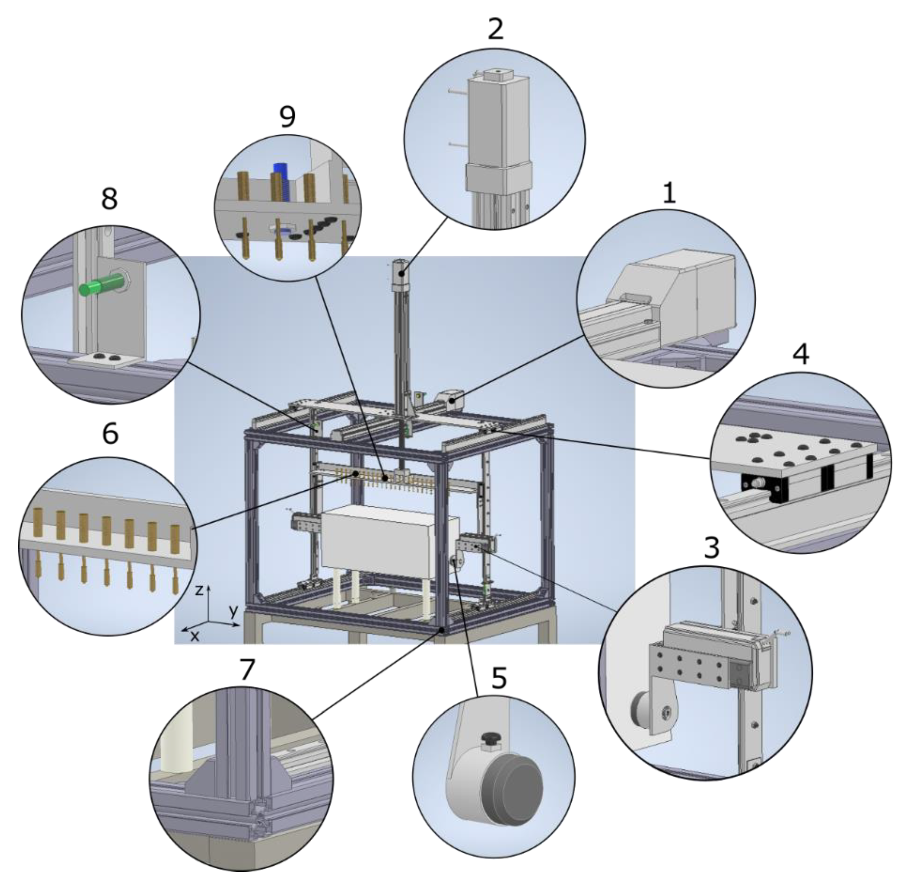
The proposed proof-of-concept machine has as its main design characteristics reliability, cost efficiency, modularity, and short-time measurements; it is shown in Figure 4.

The machine consists basically of a 3D Cartesian robot that moves two sets of measurement electrodes (electrical and ultrasonic) along the X–Y–Z coordinates.

To ensure quick 3D movements of the electrodes, without undesirable vibrations, the moving system is assembled on a sturdy base with an outer structure.

The X-axis is performed by an electric linear actuator, SMC LEFS32A-700 R5CP18, [11], with a high-precision ball screw and a moving car, reaching a positioning precision of 0.02 mm. Figure 5 shows a detailed view of the X-DOF.

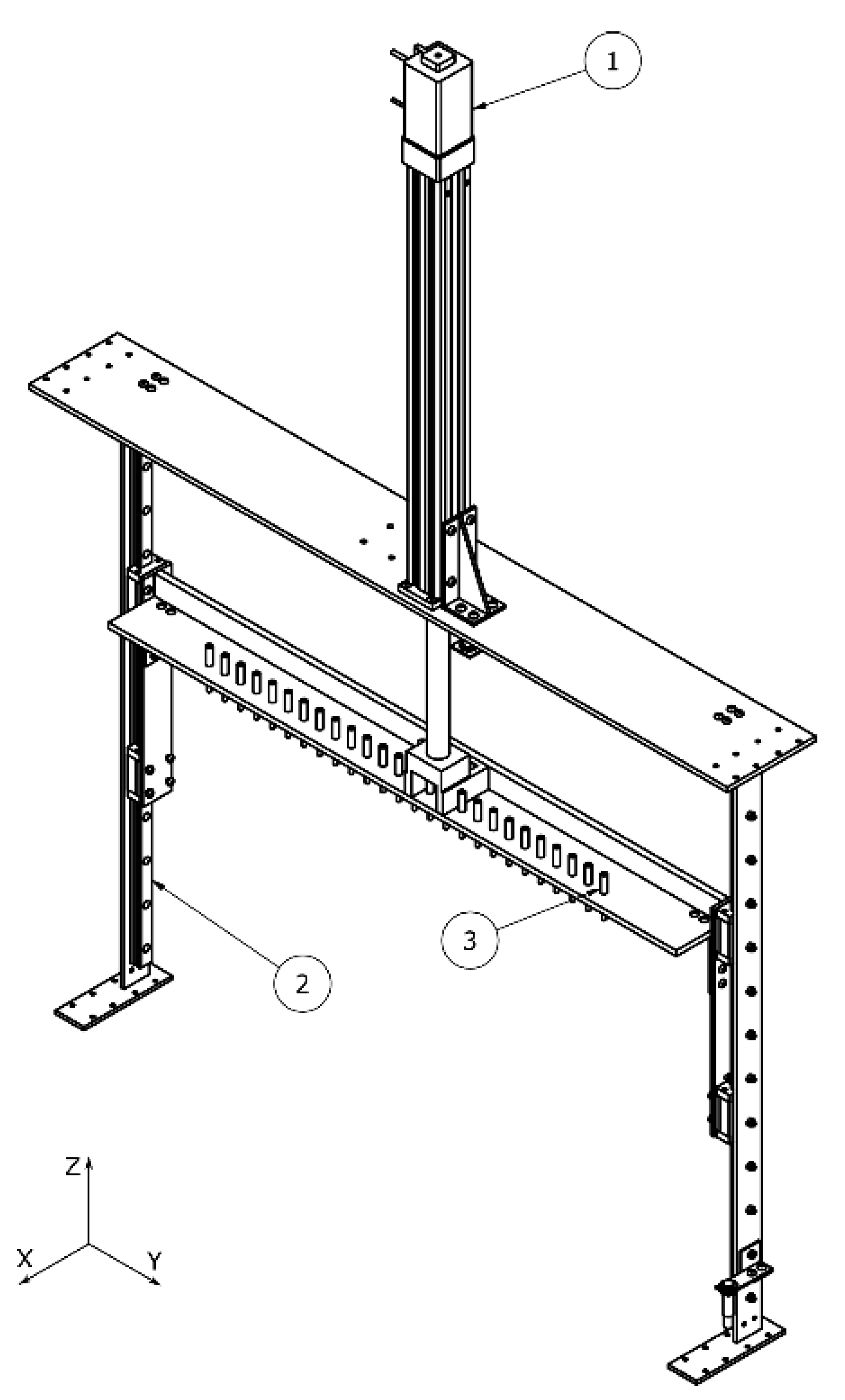
The Z-axis is performed by an electric linear rod actuator, SMC LEY32DB-450BF-R5CP18 [12], with a positioning precision of 0.02 mm. To ensure total alignment, the actuator is constrained by two more vertical Misumi SX2RL28 linear bearing guides [14]. To perform the fine search of the stone surface, along Z, an ultrasonic digital limit sensor Telemecanique XX512A1KAM8 [17] is used. Figure 6 shows a detailed view of the Z-DOF.

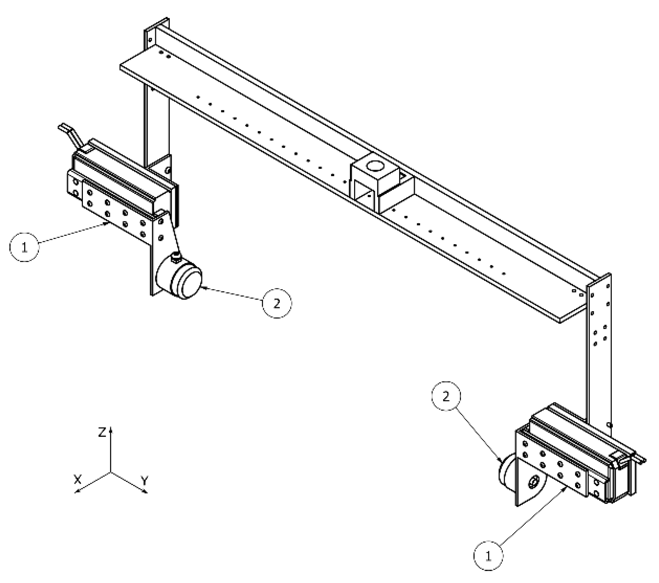
The Y-axis moves the ultrasonic sensors and is implemented by a short linear electric actuator SMC LES16RJ-75S-R5CP18 [14] and its symmetric SMC LES16LJ-75S-R5CP18 [18]. They have a short motion range and can achieve a positioning precision of 0.05 mm, being ideal for making the ultrasonic transducers contact with the block and back away to avoid damage without interfering with the system.

Finally, four inductive digital limit sensors, Telemecanique XS612B2PAL01M12 [16], are used to perform the home and to limit the linear actuators X and Z. Figure 7 shows a detailed view of the Y-DOF.

2.2. Control Design

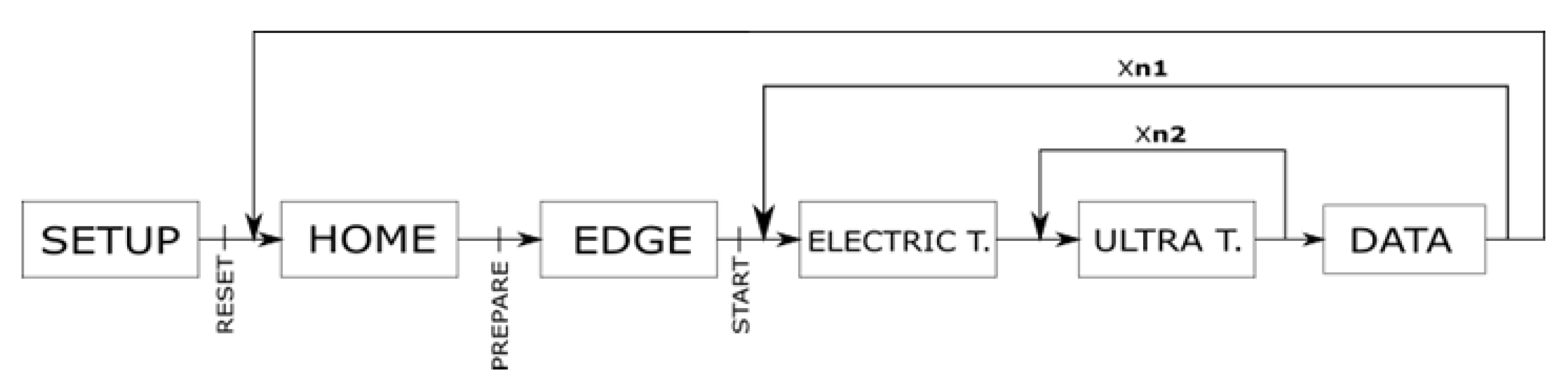
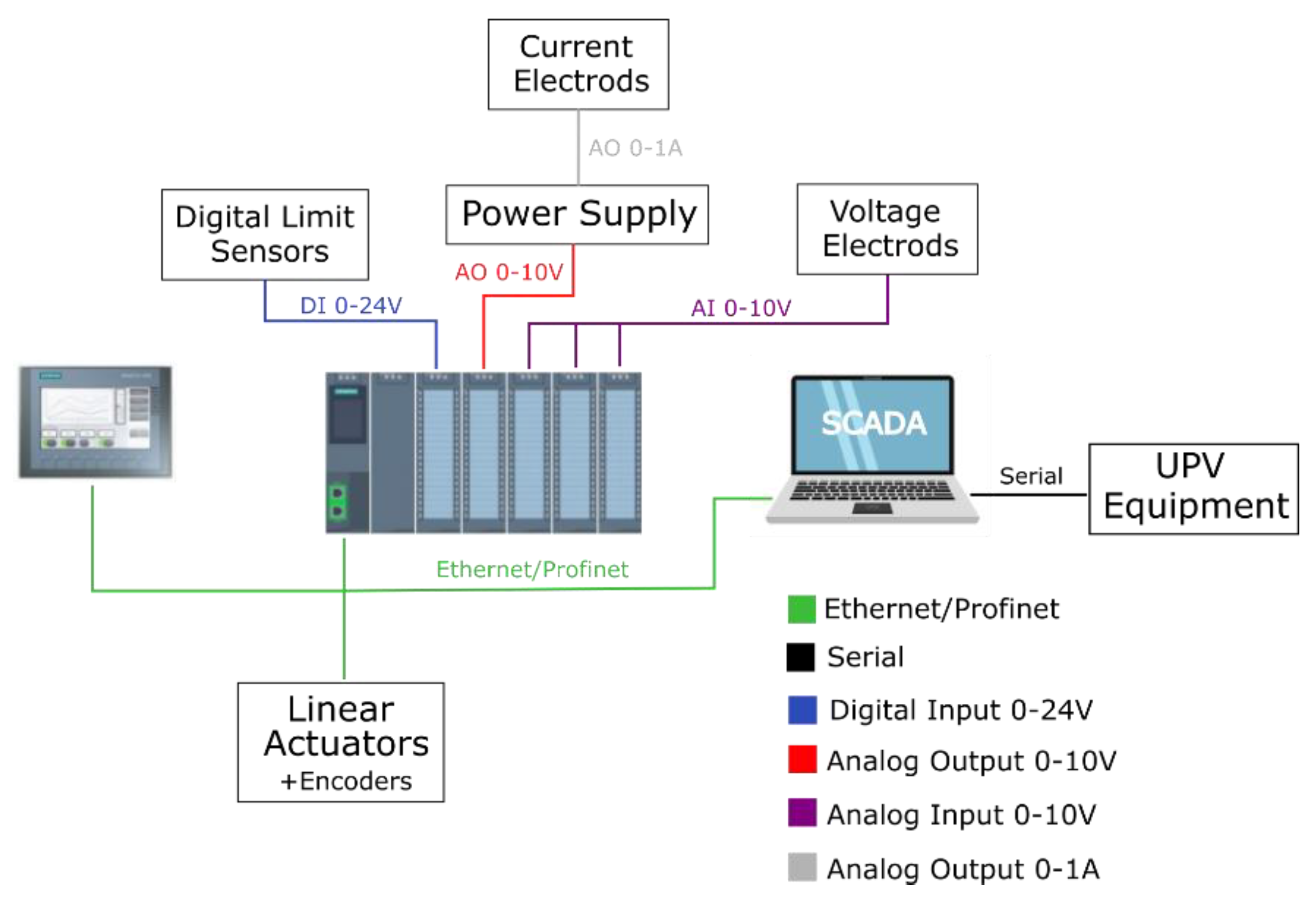
The main objective of the machine is to perform automatic electric and ultrasound tomographies. In the new developed prototype, the control is performed by two Programmable Logic Controllers (PLCs) that manage the machine operations, as briefly illustrated in the workflow presented in Figure 8.

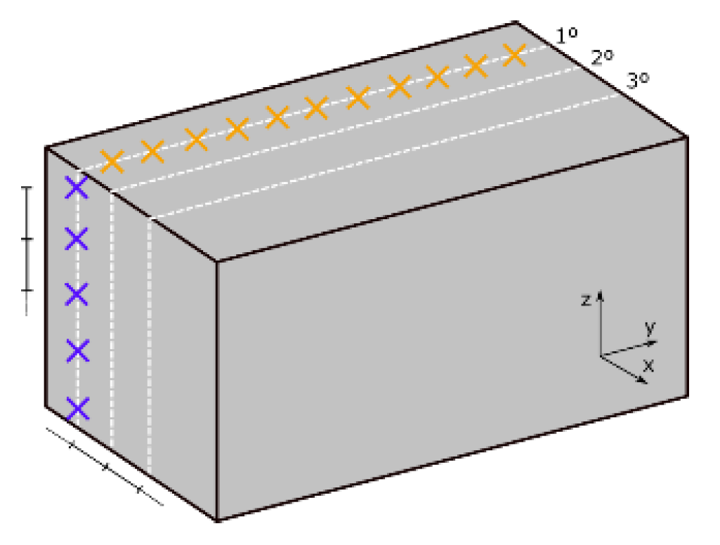
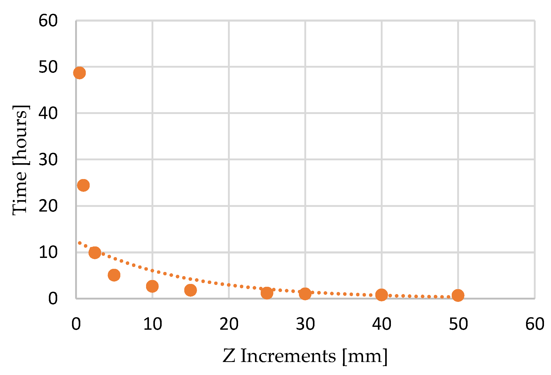
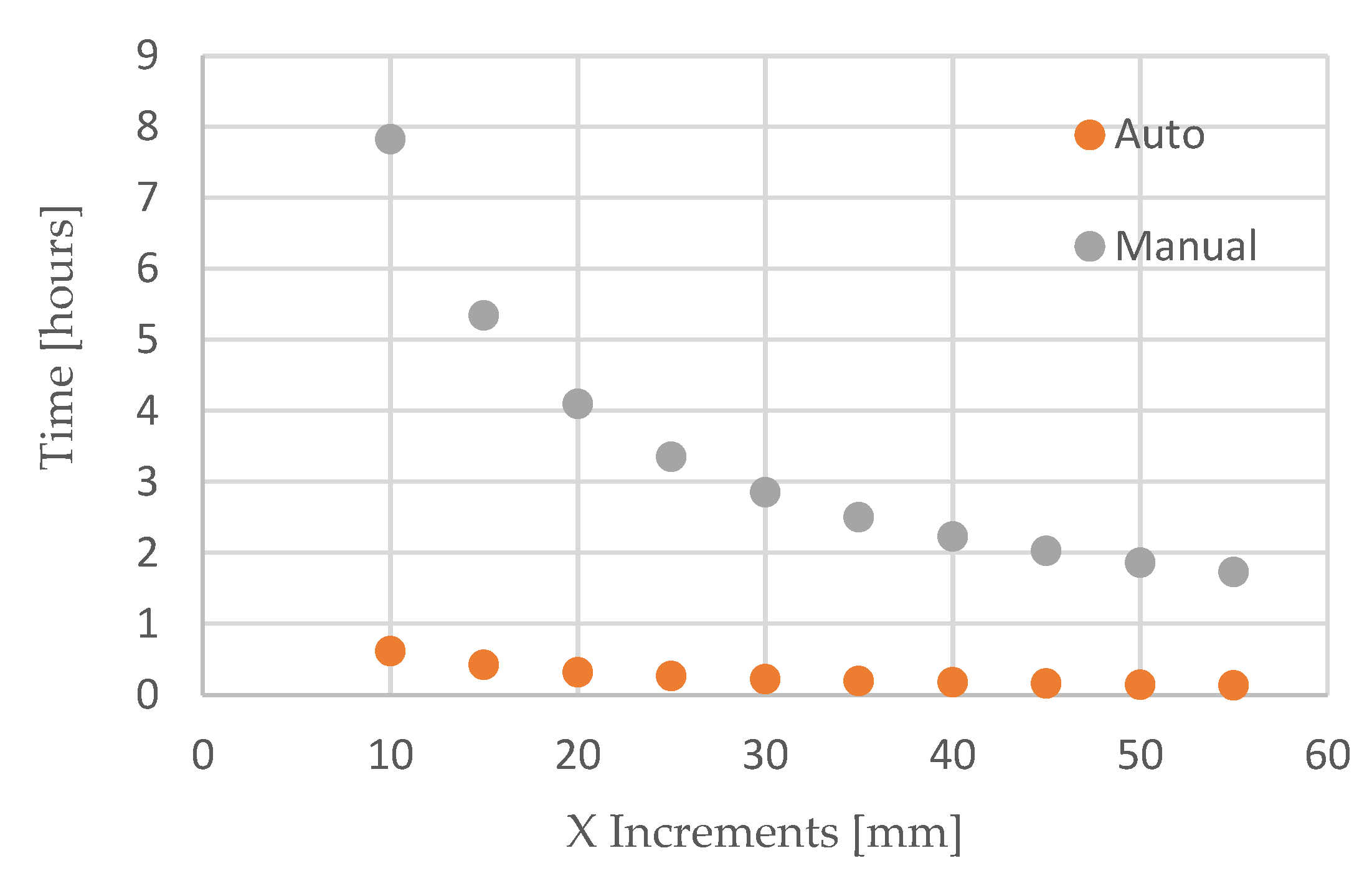
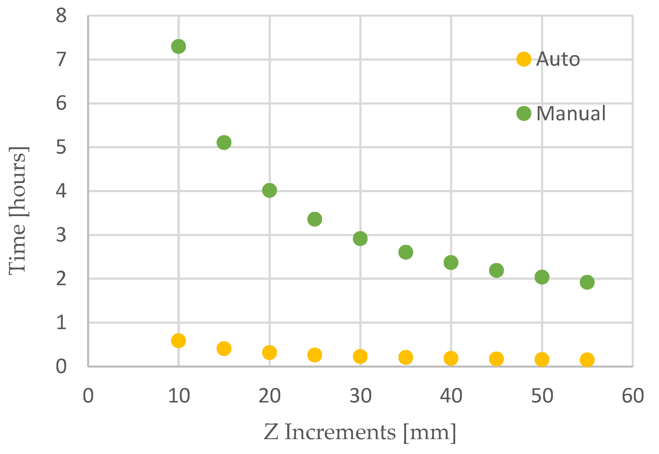
Recalling Figure 1, the stone block is divided in n₁ sections, with 5 mm increments, along the X-axis. In each section, we perform an electric tomography, as well as n₂ ultrasonic tomographies with 10 mm increments, along the Z-axis.

SETUP—This first procedure is meant to power-on and set up all the external devices that work with the PLC as well as to apply the appropriate compounds to the surfaces of the measuring devices, to guarantee suitable contact between the electrodes and the transducers with the sample surface. Being the only fully manual step, as it is just done once at the beginning of the measurements, it will not affect the overall system performance.

HOME—This automatic process returns the entire system to its original state, in which all the actuators are at their home positions and all the peripheral equipment is inactivated. This process is called every time the machine is turned on for the first time, every time a new reading is about to start, or when the system recovers from error or emergency states.

EDGE—This automatic process allows the machine to identify the edge of the stone block in order to establish a reference for the subsequent positioning of the measurement cycle.

ELECTRIC T.—In this automatic procedure, an electric tomography is performed. It is initiated by a PLC analog output that triggers the current supply (EUTRON ATR700SA 500V 1A [19]), and the subsequent voltage potential in 12 electrode pairs is read and recorded in tags. This process is made once for each stone section.

ULTRA T.—In this automatic procedure, an ultrasonic tomography is performed. A SCADA system is used to allow the connection PLC—UPV testing equipment (Proceq Pundit Lab+ [20]) with custom VBS functions (Visual Basic Scripts). This procedure triggers the ultrasonic pulse, reads the measurements, and records the data in tags. This process is performed several times (along the Z-axis) in each stone section.

DATA SAVE—Due to the significant amount of data produced for an entire block measurement, a limited number of PLC tags were created to only store information temporarily, referring to one stone section. At the end of the section measurement, using a SCADA system with custom VBS functions, all the data are exported to a new entry line in a CSV file, and all the tags are reset.

Finally, still referring to Figure 8, all functions must be called in the order they are shown in the flowchart (Figure 8), except for the HOME function that is called whenever the RESET button is pressed. The EMERGENCY button suspends all processes, stopping the actuators and deactivating the external equipment.

Table 3. Machine workflow.

Procedure	Nr.	Actions	Type
SETUP	0.1	The block sample is placed on the machine supports.	Manual
	0.2	A marble paste is applied to the electrodes and block surfaces.	Manual
	0.3	A glycerin gel is applied to the transducers and block surfaces.	Manual
	0.4	The “Proceq Pudnit Lab+” equipment is turned on and the block width (Y) is introduced by the operator.	Manual
	0.5	The “EUTRON ATR700” power supply is turned on.	Manual
	1.0	To proceed, the RESET button must be pressed.	Manual
HOME	1.1	The EUTRON power supply applies 0 V.	Automatic
	1.2	The YA actuator retracts.	Automatic
	1.3	The YB actuator retracts.	Automatic
	1.4	The Z actuator goes back to its origin.	Automatic
	1.5	The X actuator goes back to its origin.	Automatic
	2.0	Operator introduces the length (X) and the height (Z) of the stone block and the voltage value of the power supply.	Manual
	2.1	To proceed, the PREPARE button must be pressed.	Manual
	2.2	The X actuator moves to a position where the detection of the stone block surface is guaranteed.	Automatic
EDGE	2.3	The Z actuator moves down to a maximal distance of 25 mm to the block surface.	Automatic
	2.4	The X actuator moves back until the electrodes surpass the initial edge of the upper surface of the block.	Automatic
	2.5	The X actuator moves forward until the electrodes become aligned with the initial edge of the upper surface of the block.	Automatic
	3.0	To proceed, the START button must be pressed.	Manual
ELECTRIC T.	3.1	The Z actuator moves down to ensure that the electrodes are at 25 mm distance from the upper surface of the block.	Automatic
	3.2	The Z actuator moves down until the electrodes contact the upper surface of the block.	Automatic
	3.3.1	The PLC sends an analog output (0–10 V) to command the EUTRON power supply (applies a current output 0–1 A on the upper surface of the block).	Automatic
	3.3.2	The voltage detected in each electrode pair is read by the PLC and stored in tags.	Automatic
	3.3.3	The PLC sends 0V to the EUTRON power supply (current is deactivated).	Automatic
	3.4	The actuator Z moves up until the ultrasonic transducers become aligned with the upper limit of the block.	Automatic
ULTRA T.	3.5.1	The YA actuator goes forward until the transducer is pressed against the block surface.	Automatic
	3.5.2	The YB actuator goes forward until the other transducer is pressed against the block surface.	Automatic
	3.5.3	The ultrasonic tomography is initiated using the “Proceq Pundit Lab+” equipment, and the results are stored in tags.	Automatic
	3.5.4	The YA actuator retracts.	Automatic
	3.5.5	The YB actuator retracts.	Automatic
	3.5.6	The Z actuator moves down 10 mm.	Automatic
	3.5.7	The program goes back to 3.5.1 and repeats the sequence until the transducers have arrived at the lower limit of the block side surface.	Automatic
DATA SAVE	3.6	All data from both tomographies, referring to one section, are stored in a new entry line from a CSV file.	Automatic
	3.7	The X actuator moves forward 5 mm.	Automatic
	3.8	The program goes back to 3.1 and repeats the sequence until all measuring devices have arrived to the final block limit.	Automatic
	3.9	The program returns to 1.1.	Automatic

shows a detailed explanation of the individual actions contained in the above-described procedures.

According to the actions stated on the machine workflow (Table 3), the prototype hardware requirements can be defined. Figure 9 shows the prototype implementation (wiring diagram). Basically, three main controller components are selected: a PLC, an HMI, and a SCADA system.

2.3. SCADA System

This machine integrates a SIEMENS WinCC SCADA system (Supervisory Control and Data Acquisition) [21] running on a Windows PC server. This system manages three main functions: (i) interfaces the UPV test equipment and the PLC; (ii) exports the data to a CSV file via custom VBS (Visual Basic Scripts); (iii) serves as a higher-order Human–Machine Interface (HMI).

The developed SCADA main control panel is illustrated on Figure 10. Its layout reproduces the machine local HMI panel. A list of possible machine error messages is presented in

Table 4. Error messages.

Errors Messages	Causes
Error Ya0	The Ya actuator did not fully retract at the due time
Error Ya1	The Ya actuator did not fully extended at the due time
Error Yb0	The Yb actuator did not fully retract at the due time
Error Yb1	The Yb actuator did not fully extended at the due time
Error Sensor x0	The x0 sensor did not activate at the due time
Error Sensor x1	The x1 sensor did not activate at the due time
Error Sensor z0	The z0 sensor did not activate at the due time
Error Sensor z1	The z1 sensor did not activate at the due time
Error Sensor z2	The z2 sensor did not activate at the due time
Error Actuator X	The X actuator did not achieve the target location at the due time
Error Actuator Z	The Z actuator did not achieve the target location at the due time
Error Ultrasonic Tomography	The ultrasonic tomography was not completed at the expected time
Error Electric Tomography	The electric tomography was not completed at the expected time
Error Limit Sensor	One of the limit sensors was incorrectly triggered
Error Emergency Button	The emergency button was pressed

.

2.4. Laboratorial Setup

To study the viability of the developed control strategy, a laboratorial setup was created to test the behavior of the electric actuators and the digital limit sensors subjected to the developed logic control cycles, as defined in Section 2.2. Figure 11 and Figure 12 show the implemented laboratorial setup.

The laboratorial setup was implemented wih two Programable Logic Controllers (PLCs) working in tandem to simulate an industrial network. The main PLC is responsible for running the main tasks, and the other PLC runs the electric tomography.

Each actuator was simulated by using two digital bits, one for each movement direction, the electric tomography used two-input and two-output electrodes, as the objective of this prototype is testing its operational capacity (proof-of-concept setup).

The main PLC controller is the SIEMENS S7-1200 [22] with the following components:

-

CPU 1214C AC/DC/Rly (6ES7 214-1BG31-0XB0) [23]

-

14 digital inputs 0–24 V

-

10 digital outputs 0–24 V

-

2 analog inputs 0–10 V (10 bits)

-

AQ1 signal board (6ES7 232-4HA30-0XB0) [24]

-

2 analog outputs 0–10 V (12 bits)

The secondary PLC controller is the SIEMENS S7-300 [25] with the following components:

-

PS 307 2A (6ES7 307-1BA01-0AA0) [26]

-

CPU 315-2 DP (6ES7 315-2AH14-0AB0) [27]

-

CP 343-1 Lean (6GK7 343-1CX10-0XE0) [28]

-

Industrial Ethernet Communication

-

CP 342-5 (6GK7 342-5DA03-0XE0) [29]

-

PROFIBUS Communication

-

DI 8/DO 8 × 24VDC/0.5 A (6ES7 323-1BH01-0AA0) [30]

-

8 digital inputs 0–24 V

-

8 digital outputs 0–24 V

-

AI 4/AO 2 × 8BIT (6ES7 334-0CE01-0AA0) [31]

-

4 analog input 0–10 V (8 bits)

-

2 analog outputs 0–10 V (8 bits)

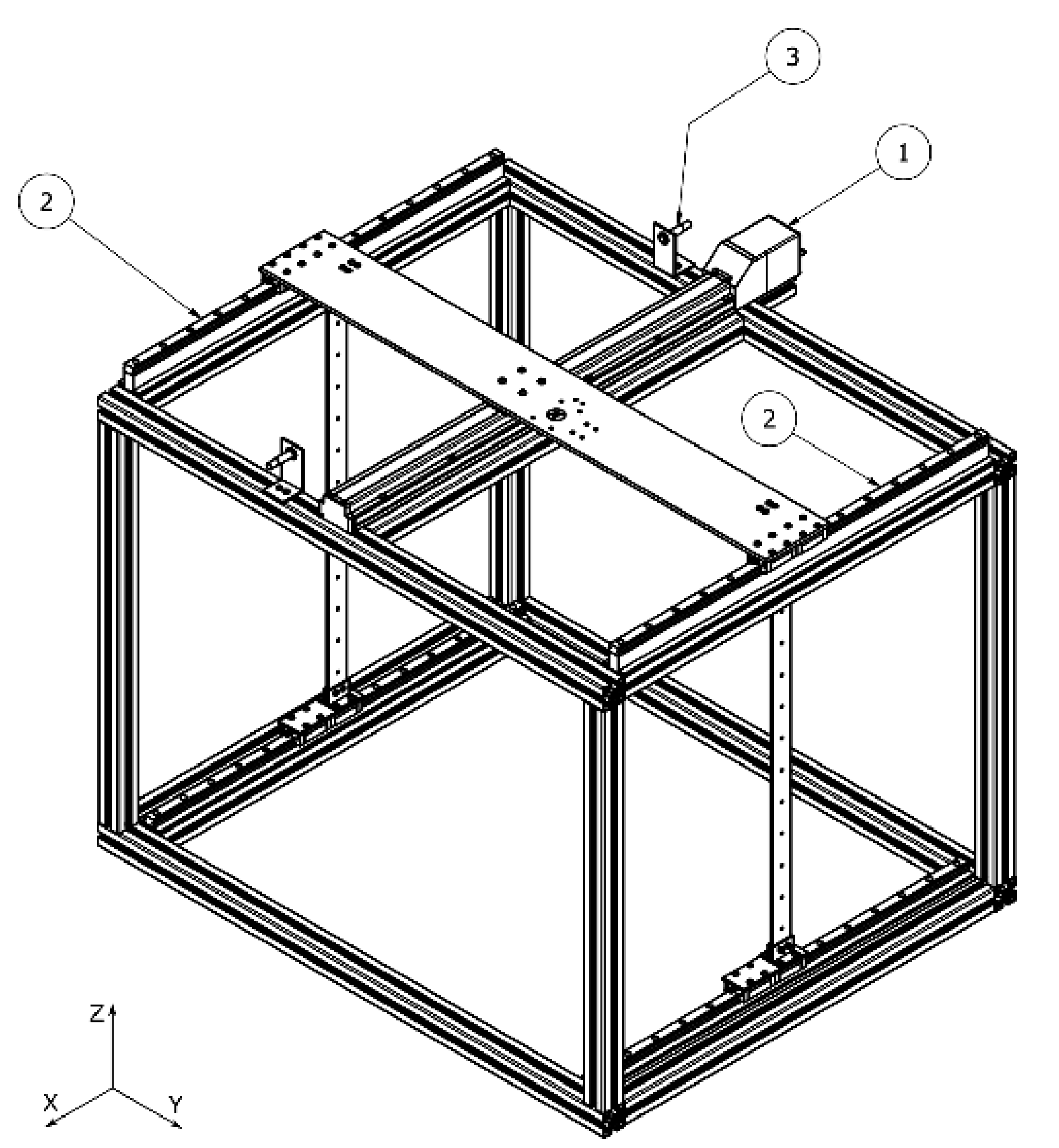
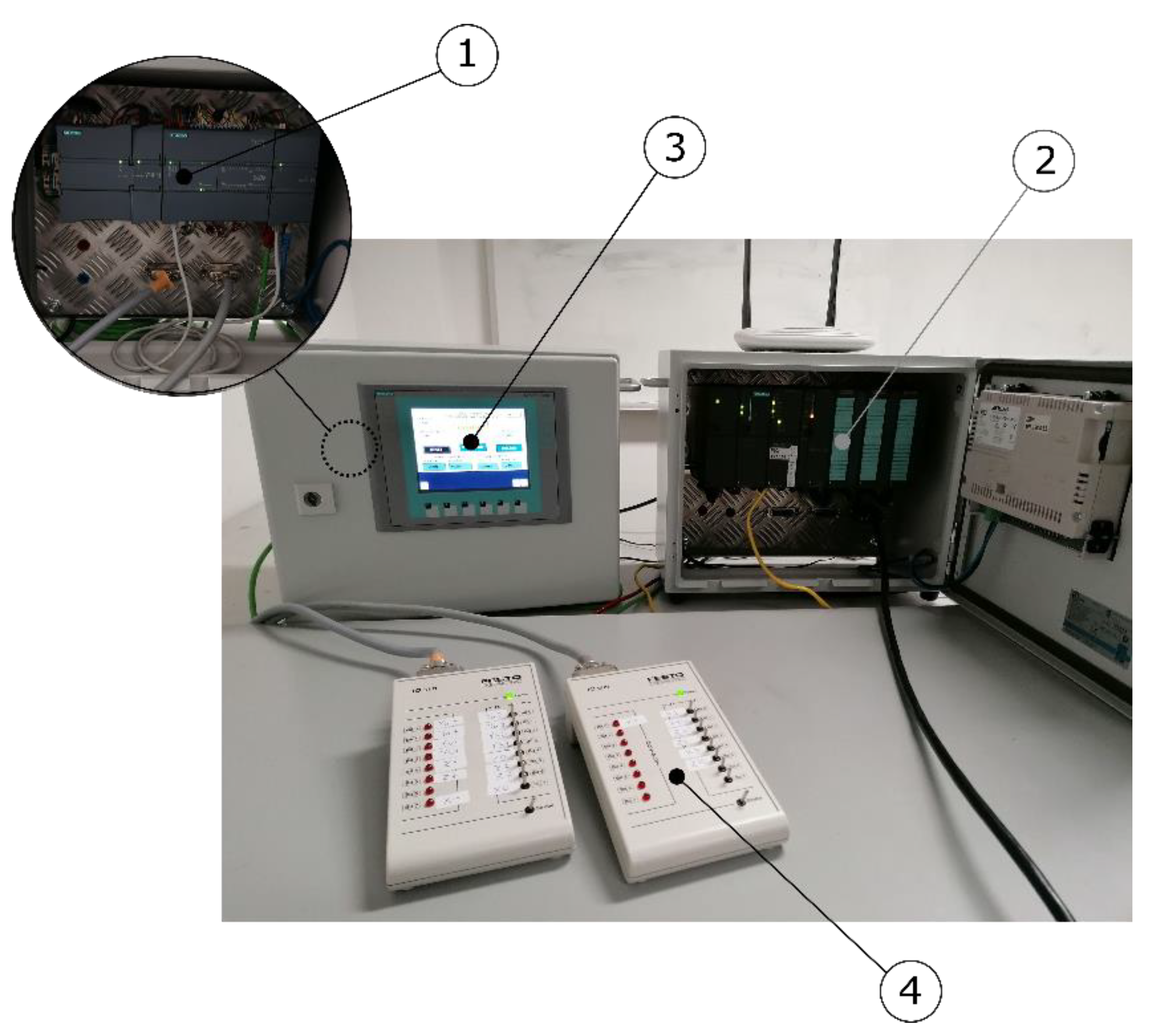
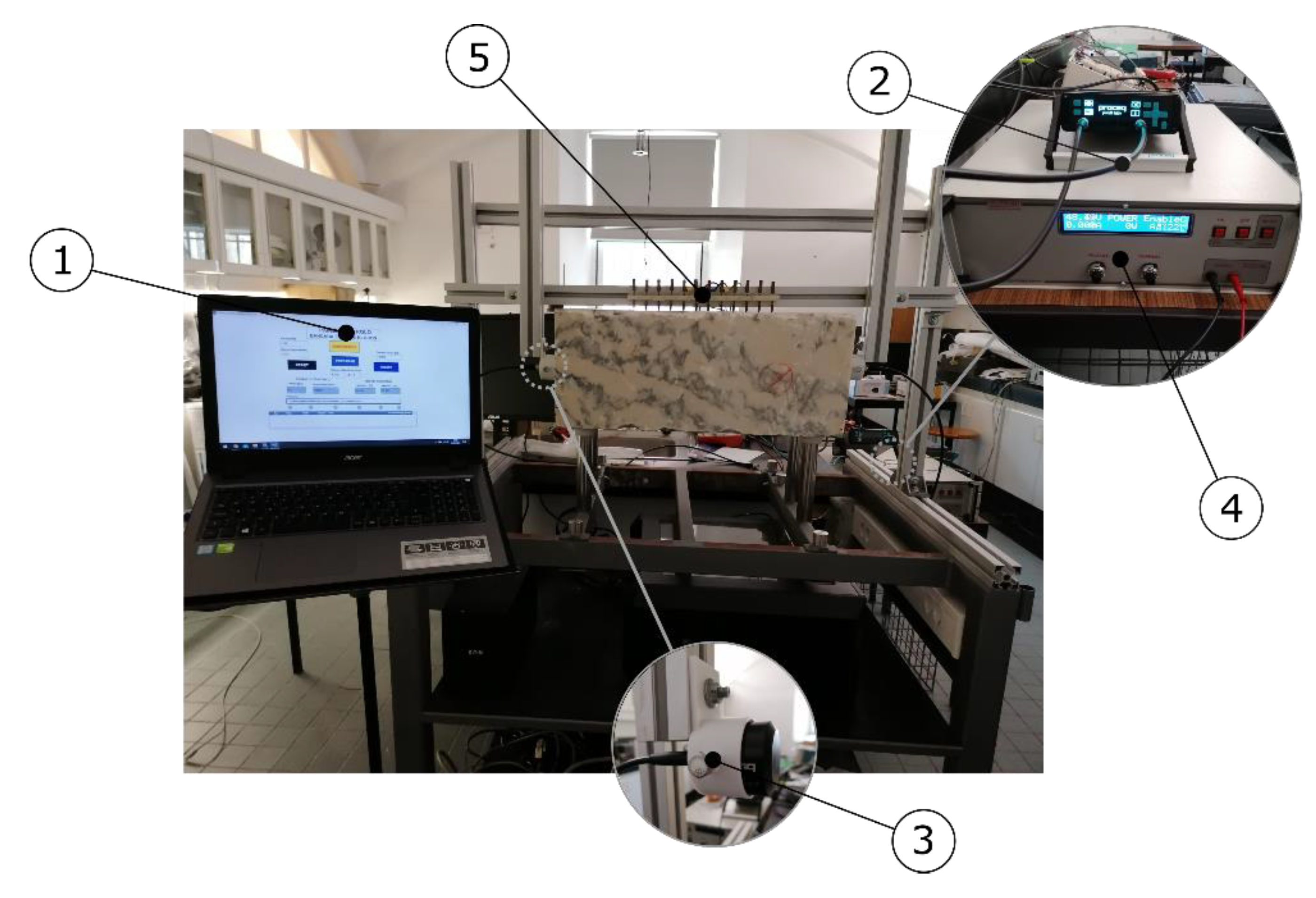
The SIEMENS KTP600 Basic Color PN (6AV6647-0AD11-3AX0) [32] is used in the prototype as the Human–Machine Interface (HMI)–the (3) in Figure 12.

A SIEMENS WinCC Advanced SCADA system [21] is integrated in the prototype–the (1) in Figure 11-to fulfill three objectives: (i) online supervision and control of the entire machine; (ii) management of the communication between both PLCs—via VBS (Visual Basic Scripts); (iii) bridge the communication between the UPV test equipment and the main controller.

Ultrasonic tomography uses the Proceq Pundit Lab+ test equipment [20]–the (2) in Figure 11-and two ultrasonic 54 kHz transducers–the (3) in Figure 11.

Finally, electric resistivity tomography uses the EUTRON ATR700SA [19]–the (4) in Figure 11—(4)) and test brass-electrodes with spring-contact tips to ensure effective electrical contact between testing surfaces–the (5) in Figure 11.

2.4.1. VBS Functions—Integration PLC/Proceq Pundit Lab+

The UPV test equipment “Proceq Pundit Lab+” [20], can be connected to a PC, via its COM port, using the serial communication with the following parameters:

-

115,200 Baud Rate

-

8 Data Bit

-

1 Stop Bit

-

No parity

This device has a communication protocol based on a series of hexadecimal commands in a pre-defined order.

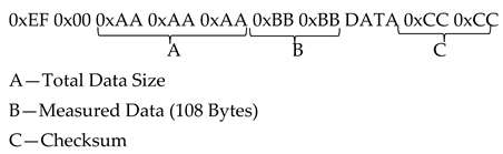
After each measurement, the equipment sends the resulting data as well as some extra information in a sequence of hexadecimal blocks [20]. The measurement data are composed by 108 bytes added by seven more information bytes at the beginning and two more Checksum bytes at the end (assuming there is no sample curve); the equipment will send a total of 117 bytes.

Relevant information for this study is the following data [20]: (i) propagation time (bytes 29 to 32); (ii) general absolute position (bytes 36 to 39); (iii) propagation velocity (bytes 37 to 40); and (iv) general absolute position (bytes 44 to 47).

The communication between the PLC and the Pundit equipment is assured by the SIEMENS WinCC SCADA system with custom VBS (Visual Basic Scripts) to allow serial communication (send and receive hexadecimal data). The “Microsoft Communications Control” Version 6.0 ActiveX control developed by Microsoft was used to perform this task.

Four custom scripts were developed to handle the serial communication and the data flow, namely: Open_S(); Send(); Receive(); and Close_S(). A brief explanation of these scripts follows.

“Open_S()”—Script that uses the MSComm object to define the serial communication parameters according to the ones used by the Pundit Lab+ as well as the COM port where the device is connected and the start of the communication.

“Send()”—Script that, using the MSComm object, is responsible for sending the hexadecimal data blocks to trigger the measurement of the UPV device.

“Receive()”—Script that reads and processes the entire buffer received from the UPV device. Starts by identifying the bytes that records the velocity and time information. After the acquisition, the data are converted to a decimal base for easier interpretation.

“Close_S()”—Script whose only objective is to fully close the serial communication.

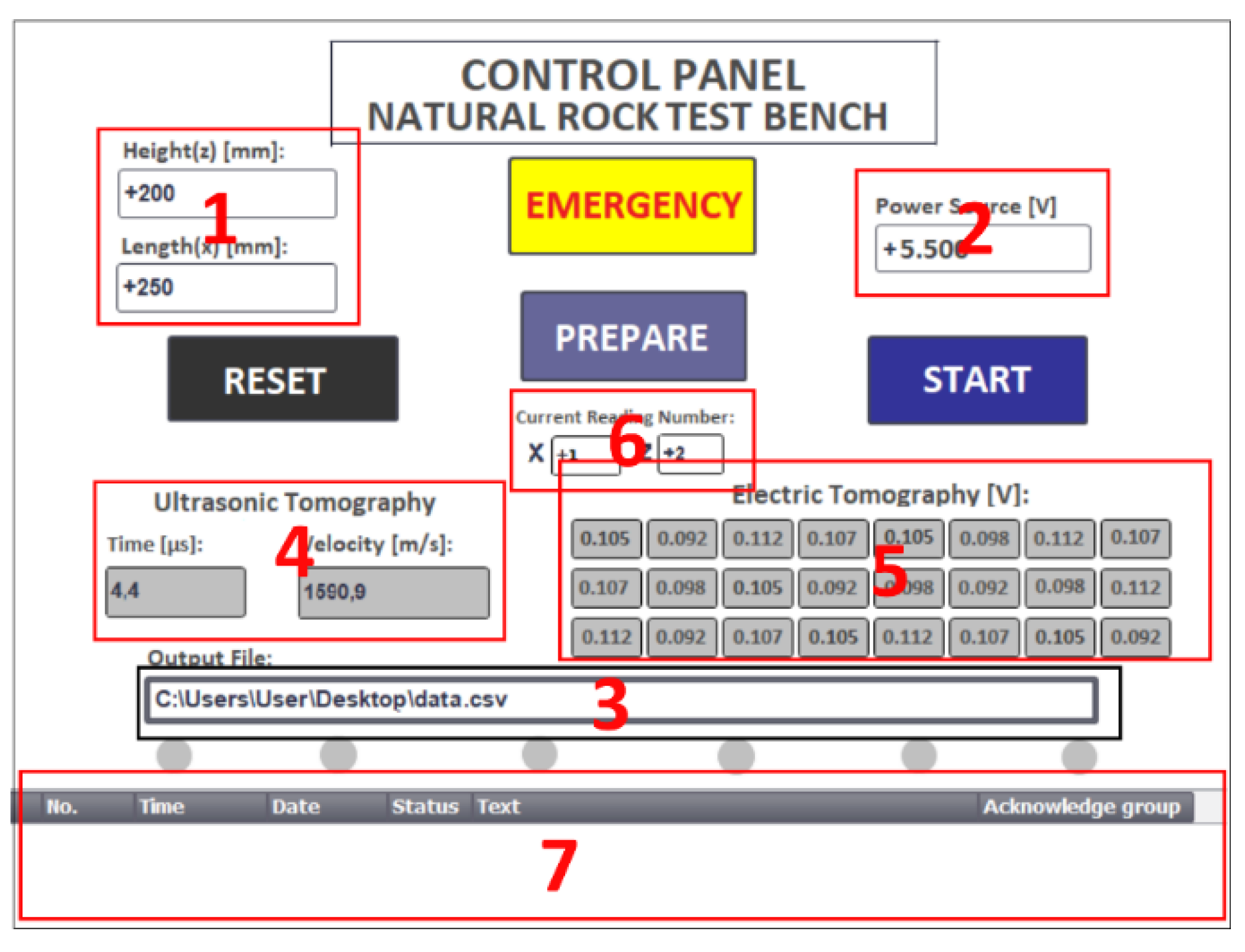
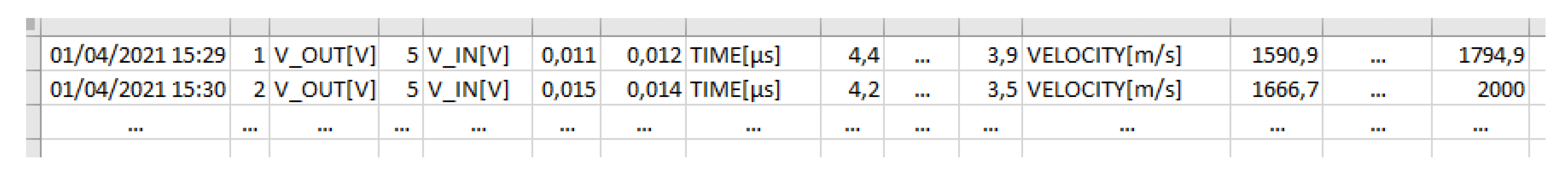
2.4.2. Data Exporting Script

To automatically save the measurement values on a standard form, a custom VBS (Visual Basic Script) was developed to create a new CSV (Comma-Separated Values) file, whose name and location are customizable by the operator—see Figure 13. Each line begins by the context information: date and time, section number, and output voltage value. The following data refer to the measurements sequence: 2 voltage values from the electrodes, 26 propagation times, and 26 propagation velocities. The 26 propagation times and velocities refer to the ultrasonic tomography (the experimental setup has a limit of 26 measurements per section).

3. Analysis and Results

In this section, a comparison between the new developed automatic machine and the actual manual measuring procedure is presented. As the new developed system consists of a proof-of-concept prototype, the values used in this study are taken mainly from the suppliers’ datasheets.

3.1. Accuracy

3.1.1. Ultrasonic Tomography

To compare the accuracy of the measurements from both procedures (automatic and manual), a reference stone bock—ZX section, 250 mm width and 250 mm height—was considered, with a limited number of veins with different propagation velocities in known locations (Figure 14). Applying both procedures on this reference section, the accuracy of the results can be comparatively evaluated.

The used criterium to compare both procedures considers the following: (i) each pixel of the grid represents a tomography; (ii) a pixel whose dimension is at least 85% inside the area of a vein is accepted as a detected vein.

Regarding the manual procedure, two cases were considered: (1) 10 × 10 grid (Figure 15), which is a regular measuring grid achievable by a skilled operator, and (2) the best manual case scenario of a 15 × 15 grid (Figure 16), which is considered as the highest accuracy that can be performed by manual measurements.

Regarding the new developed automatic procedure, it is considered a 41 × 21 grid (Figure 17), whose accuracy is allowed by the prototype setup.

Table 5. Ultrasonic tomography—accuracy results.

Procedure	Grid	$\mathbf{Total} \mathbf{Vein} \mathbf{Area} \left[{\mathbf{mm}}^2\right]$	$\mathbf{Total} \mathbf{Accurately} \mathbf{Detect} \mathbf{Area} \left[{\mathbf{mm}}^2\right]$	Percentage [%]
Manual skill	10 × 10	14,610.8	5625.0	38.5
Manual best	15 × 15		7777.8	53.2
Automatic	41 × 21		11,977.4	82.0

shows the comparative accuracy in detecting stone veins by three significant grid dimensions (automatic and manual measuring procedures).

Analyzing the numerical results, as shown in Table 5, it is possible to detect a major difference between the automatic and manual procedures. The manual procedures show a very low capacity of veins detection when compared with the automatic procedure. In fact, both manual grids (10 × 10 and 15 × 15) detect at the highest detection capacity only 53.2% of the target area, while the automatic procedure (grid 41 × 21) arrives to a detection rate of 82.0%. The proposed automatic measurement procedure can easily achieve much finer grids that will result in much more accurate results. In fact, the smaller veins are not detected by the coarser grid (10 × 10) and only barely detected by the 15 × 15 grid.

3.1.2. Electric Resistivity Tomography

Following the same criterium used for the accuracy evaluation of ultrasonic tomography (Section 3.1.1), we now consider a reference stone bock—XY section, 600 mm width, and 250 mm height—with a limited number of veins (Figure 18). Applying both procedures (automatic and manual) on this reference section, the accuracy of the results can be comparatively evaluated.

Regarding the manual procedure, two cases were considered: (1) 14 × 10 grid (Figure 19), which is a regular measuring grid achievable by a skilled operator and (2) 14 × 15 grid (Figure 20), the manual best case scenario, which is considered the highest accuracy that can be performed by manual measurements.

Regarding the new developed automatic procedure, we considered a 20 × 41 grid (Figure 21), whose accuracy is allowed by the current prototype setup.

Table 6. Electric tomography—accuracy results.

Procedure	Grid	$\mathbf{Total} \mathbf{Vein} \mathbf{Area} \left[{\mathbf{mm}}^2\right]$	$\mathbf{Total} \mathbf{Accurately} \mathbf{Detect} \mathbf{Area} \left[{\mathbf{mm}}^2\right]$	Percentage [%]
Manual skill	14 × 10	37,538.3	15,000.0	40.0
Manual best	14 × 15		22,142.9	59.0
Automatic	20 × 41		31,646.3	84.3

shows the comparative accuracy in detecting stone veins by three significant grid dimensions (automatic and manual measuring procedures).

Analyzing the numerical results shown in Table 6, it is possible to detect a major difference between the automatic and manual procedures. The manual procedures show a very low capacity of veins detection when compared with the automatic procedure. In fact, both manual grids (14 × 10 and 14 × 15) detect at the highest detection capacity, only 59% of the target area, while the automatic procedure (20 × 41 grid) arrives to a detection rate of 84.3%. The proposed automatic measurement procedure can easily achieve much finer grids that will result in much more accurate results. Visually, we can see that the automatic procedure provided accurate results, maintaining most of the vein’s original shapes and dimensions.

Finally, it is worth mentioning that these results assume that the reading’s precision is 100%, which can be a good approximation for the automatic system but not for the manual one, resulting in even poorer results for the manual procedures.

3.2. Measurement Time

In addition to the accuracy improvement, another great advantage of the automatic procedure regarding manual measurements is the significant time savings and correspondent economic savings to obtain ultrasonic and electric tomographies. The calculations done in this section assume the manufacturers data specifications [33,34,35] for axis movements. These reference values are shown in

Table 7. Actuators speeds.

Axis	Automatic System
X	100 mm/s
Z	70 mm/s
Y	40 mm/s

.

An important parameter that greatly influences the automatic measurement time is the selection of the axis increment to take subsequent measurements. Figure 22 and Figure 23 show the relation between axis increments and duration of a tomography, assuming a 250 × 250 × 600 mm stone block and the axis actuators moving at correspondent constant velocity (see Table 7).

In both graphs, it is seen that the time exponentially increases as the increment size becomes smaller.

Finally, Figure 24 and Figure 25 show a comparative performance analysis between the manual and the automatic measurement procedures. Both figures consider measured manual times and simulated automatic times (according to manufacturer data specifications—see Table 7). Both measurement procedures (manual and automatic) were performed on the reference stone block (250 × 250 × 600 mm).

Figure 24 and Figure 25 clearly show the significant superior performance of the automatic measurement when compared with the manual procedure. The finer the increments, the greater the performance difference, reaching seven hours difference for automatic standard 10 mm axis increments.

3.3. Measurement Precision

The accuracy of the automatic machine is considered as given by the technical specifications of the manufacturer’s axis [33,34,35]. These data specifications are summarized in

Table 8. Manufacturer’s axis accuracy specs.

Axis	Automatic System
X	0.02 mm
Z	0.02 mm
Y	0.05 mm

.

Regarding the manual measurement, the average precision depends on the characteristics of the operator, namely the qualification, experience, and skill. Then, a typical number is hard to identify, but on average, a highly qualified operator can reach a precision of about 5 mm (common to all directions—axis).

4. Conclusions

The aim of this work was to improve the data analytics of the marble industry sector with the focus on increasing sustainability and competitivity. With this objective, an existing laboratorial structure used to perform manual electric resistivity and ultrasonic tomographies on stone blocks was redesigned. The data obtained from the tomographies are later used on simulations of the internal structure of the measured stone blocks.

Trying to improve the existing procedures for collecting stone information and data exporting, a novel approach to the current methodology was developed by the authors. The proposed system presents sound advantages when compared to the previous methodology: namely, (i) high accuracy due to new automatic positioning system; (ii) no need for highly skilled operators to process measurements; (iii) measurements are much easier to derive, and results are quickly delivered.

The new developed machine consists basically of a 3D cartesian robot that moves two sets of measurement electrodes (electrical and ultrasonic) along X–Y–Z coordinates. This machine integrates a SIEMENS WinCC SCADA system (Supervisory Control and Data Acquisition) running on a Windows PC server that performs two main tasks: management of the operative PLC and exporting digital results for further data storage.

In order to evaluate the new developed machine performance, a comparison between the new automatic process and the actual manual measuring procedure was established. The study shows that manual procedures show a very low accuracy when compared with the developed automatic procedure. In addition to the accuracy improvement, another great advantage of the automatic measurements is the significant time savings and correspondent economic savings to obtain ultrasonic and electric tomographies.

Finally, the new design and implementation of the laboratorial proof-of-concept demonstrates that the systematic application of this concept can be extended to industrial processes, supporting decision making to improve the cutting of stone blocks, bringing economic value to the business.