Article

Homogenized Balance Equations for Nonlinear Poroelastic Composites

School of Mathematics and Statistics, Mathematics and Statistics Building, University of Glasgow, Glasgow G12 8QQ, UK
*
Author to whom correspondence should be addressed.
Appl. Sci. 2021, 11(14), 6611; https://doi.org/10.3390/app11146611
Submission received: 12 May 2021 / Revised: 1 July 2021 / Accepted: 6 July 2021 / Published: 19 July 2021

Abstract

:
Within this work, we upscale the equations that describe the pore-scale behaviour of nonlinear porous elastic composites, using the asymptotic homogenization technique in order to derive the macroscale effective governing equations. A porous hyperelastic composite can be thought of as being comprised of a matrix interacting with a number of subphases and percolated by a fluid flowing in the pores (which is chosen to be Newtonian and incompressible here). A general nonlinear macroscale model is derived and is then specified for a particular choice of strain energy function, namely the de Saint-Venant function. This leads to a macroscale system of PDEs, which is of poroelastic type with additional terms and transformations to account for the nonlinear behaviour of the material. Our new porohyperelastic-type model describes the effective behaviour of nonlinear porous composites by prescribing the stress balance equations, the conservation of mass and Darcy’s law. The coefficients of these macroscale equations encode the detailed microstructure of the material and are to be found by solving pore-scale differential problems. The model reduces to the following limit cases of (a) linear poroelastic composites when the deformation gradient approaches the identity, (b) nonlinear composites when there are no pores and (c) nonlinear poroelasticity when only the matrix–fluid interaction is considered. This model is applicable when the interactions between various hyperelastic solid phases occur at the pore-scale, as in biological tissues such as artery walls, the myocardium, lungs and liver.

1. Introduction

The theory of poroelasticity can be used to describe the effective mechanical behaviour of porous elastic materials with fluid flowing in the pores. This modelling approach can be applied to materials undergoing both linear and nonlinear deformations. The linear theory was developed by Biot in [1,2,3,4]. Due to the desire to apply poroelasticity to biological tissues, the theory was adapted to nonlinearities in [5,6,7,8]. The poroelastic modelling framework is applicable to a wide variety of physical scenarios, in particular to biological tissues, where the deformations are in general nonlinear. For example, a poroelastic approach has been taken to model organs such as lungs (see, e.g., [9]) and to consider the perfused myocardium [10,11]. Poroelasticity has also been applied to studying the artery walls (see, e.g., [12,13]). Nonlinear poroelasticity has also been applied to modelling tumour growth [14] and in imaging to locate tumours in an incompressible medium [15]. It is also of interest in porous thermoelasticity (see [16]). For a general overview of the micromechanics of porous media, we refer the reader to [17], where an overview of upscaling techniques, the linear theory of porous media and also the extension of the analysis to the nonlinear homogenization of a large range of scenarios including strength homogenization, nonsaturated microporomechanics, microporoplasticity and microporofracture and microporodamage theory were discussed.
We consider hyperelastic deformable porous media, and in general, these types of materials have a variety of structural features characterised over multiple scales. We have a scale (called the pore-scale) where the interactions between the fluid and the solid take place, and this scale is much smaller than the scale at which we describe the whole material (which is called the macroscale).
The coupled fluid–structure balance equations that describe the material on the pore-scale can be used in an upscaling process to obtain the macroscale governing equations of a poroelastic material. The upscaling process can be carried out by a variety of homogenization techniques. These homogenization techniques include effective medium theory, mixture theory, volume averaging and asymptotic homogenization. These techniques were discussed and described in [18,19].
We develop our analysis by means of the asymptotic homogenization technique [20,21,22,23]. This technique requires a sharp length-scale separation, between the pore-scale and the macroscale, to enable the decoupling of spatial variations that exist in the system. This technique expresses the relevant fields from the pore-scale fluid–structure interaction problem as power series of the ratio between the two different typical length scales. The balance equations obtained via this method describe the effective behaviour of the material in the homogenized macroscale domain. A key feature of this technique is that the coefficients of the macroscale model encode information about the microstructure of the material, and they are to be computed by solving differential problems at the pore-scale. In the literature, the asymptotic homogenization technique has been applied to various physical systems. For example, the asymptotic homogenization technique has been used to derive Biot’s poroelasticity (see [24,25]) and extended to study vascularised poroelastic materials [26], poroelastic composites [27] and modelling of the bones [28].
In the asymptotic homogenization literature, the majority of the applications focus on linearised balance equations. This is due to the fact that in the linearised case, it is possible to fully decouple the pore-scale and the macroscale (under some simplifying assumptions). This decoupling then leads to a large reduction in the computational complexity of the system. In the literature, the homogenization of systems involving nonlinear mechanics is generally carried out by other homogenization techniques, such as average field techniques (see, e.g., [29,30] and the references therein). These other techniques do not provide a precise description of the model coefficients in the way that the asymptotic homogenization technique can and, instead, provide bounds for the model coefficients. There are currently only a few examples of using asymptotic homogenization in situations where the material undergoes large deformations. In [31], the effective poroelastic model of Biot was extended to a nonlinear Biot model that includes pore-scale deformation. In [32], a system of effective equations that describe the flow, elastic deformation and transport in an active medium was derived. The authors considered the spatial homogenization of a coupled transport and fluid–structure interaction model. In [33], the asymptotic homogenization technique was applied to the equations that describe the dynamics of a heterogeneous material with an evolving microstructure to obtain a set of effective equations. The heterogeneous body is assumed to be composed of two hyperelastic materials, and the evolution of the microstructure is through plastic-like distortions.
We investigate materials that are subject to large deformations that have the underlying microstructure comprised of both a hyperelastic-fluid-filled porous matrix and a number of embedded hyperelastic subphases (fibres or inclusions). We then assume that both the matrix and the subphases interact with each other and the fluid at the pore-scale. This type of structure can be described as a poroelastic composite material that undergoes large deformations. For example, this is applicable to artery walls, which can be considered as a composite nonlinear elastic material consisting of a matrix with two families of symmetrically arranged embedded collagen and elastin fibres as well as fibroblast cells that interact with the fluid that is flowing in the pores [12,34,35,36,37]. If we wish to consider the artery walls in our framework, then the matrix can be identified with our matrix in the model, and the fibres and fibroblast cells could all be considered as the elastic subphases that are embedded in the matrix. The fluid in this setting would be the water that flows in the pores of the matrix. This modelling approach is applicable to the myocardium in the heart, which is a nonlinear elastic porous structure that consists of a matrix with muscle cells, fibroblasts, collagen fibres and embedded blood vessels [10,11,38]. Again, here, the various muscle cells, fibroblasts and fibres would all be the elastic subphases embedded in the matrix. By considering these systems as poroelastic composites, we are able to account for the mechanical contribution of each of the various phases individually.
Here, we generalise [27] to account for nonlinear deformations by using the asymptotic homogenization technique to upscale the interaction between a hyperelastic porous matrix where there is an incompressible Newtonian fluid flowing in the pores and a number of embedded hyperelastic subphases. We make the assumption that both the hyperelastic matrix and subphases interact with the fluid that is flowing in the pores. We assume that the length scale where the individual hyperelastic subphases are clearly visible from the surrounding matrix is comparable to the pore size. We therefore determine that this scale will be the pore-scale of the material, that is the distance between adjacent subphases is comparable with the size of the pores. This length is assumed to be much smaller than the size of the whole domain, which is denoted the macroscale. The upscaling process is then used taking into account the continuity of the stresses and elastic displacements across the interfaces between the matrix and the subphases, as well as the continuity of the stresses and velocities across the interfaces between the fluid and solid domains. Furthermore, an appropriate coordinate transformation is carried out on some quantities to formulate the full problem in the undeformed/reference configuration, i.e., by solely using Lagrangian coordinates. The resulting system of governing equations is of poroelastic type and is a generalization of the formulations for (a) multiphase elastoplastic composites [33] in the limit of no plastic distortions and (b) the formulations for hyperelastic porous media [31] in the limit of only one elastic phase. It is also a natural extension to the formulation for linear poroelastic composites [27]. All three of these formulations are recovered as particular cases by assuming that: (a) our matrix is not porous; (b) that no elastic phase other than the matrix is present; and (c) by performing a linearisation. The coefficients of the model encode the properties of the microstructure and are computed by solving local differential problems.
The paper is organised as follows. In Section 2, we formulate the fluid–structure interaction problem that characterises the behaviour of the hyperelastic porous matrix, the hyperelastic subphases and the fluid flowing in the pores. We also perform a change of coordinates, which allows the fluid–structure interaction problem to be formulated in the reference configuration. In Section 3, we apply the asymptotic homogenization technique to the system of PDEs that were described in Section 2 and determine the new model that describes the effective macroscale mechanical behaviour of nonlinear poroelastic composites. In Section 4, we discuss the general nonlinear macroscale model before prescribing a specific strain energy function, namely the de Saint-Venant, for the material and then give a physical interpretation of the novel terms. We also consider particular cases for our new model and are able to obtain previously known models from the literature. Section 5 concludes our work by highlighting and discussing the limitations of the current model and by providing further directions in which the model could be extended for particular biological applications.

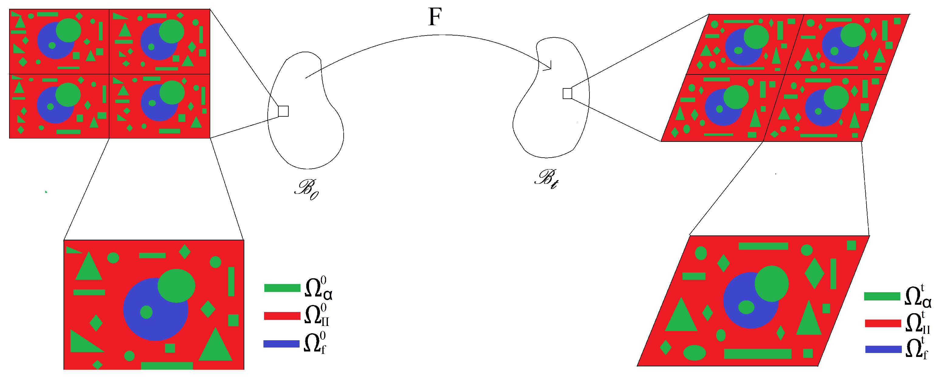
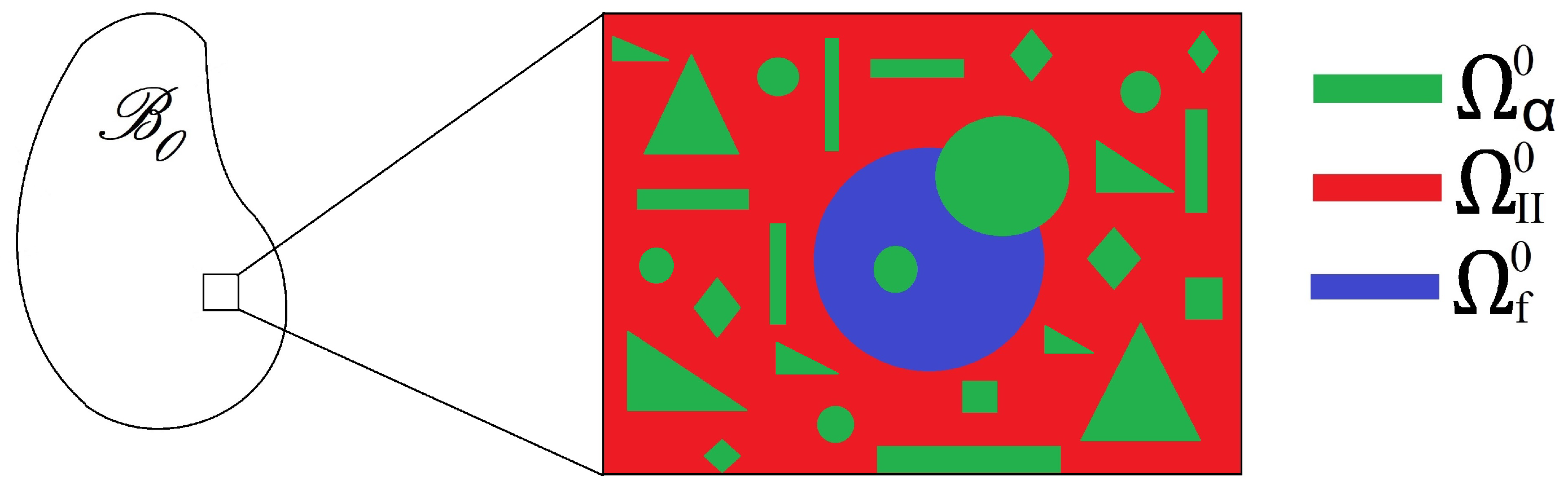
2. Formulation of the Fluid–Structure Interaction Problem

We assume that we have a continuum body that is not subject to any surface or body forces to have a reference configuration, which we denote by B 0 R 3 . The body B 0 has a periodic microstructure that consists of the union of a porous hyperelastic matrix Ω II 0 , an interconnected fluid compartment Ω f 0 and a set Ω I 0 of K disjoint hyperelastic subphases Ω α 0 , where:
Ω I 0 = α = 1 K Ω α 0 ,
and Ω ¯ 0 = Ω ¯ I 0 Ω ¯ II 0 Ω ¯ f 0 . We note that when any domain, interface or normal vector has the superscript 0 then it is in the reference configuration. We provide a sketch of this structure as shown in Figure 1. The body undergoes a deformation described by the deformation function χ , and the deformed body is denoted by B t . Each point x B t is such that x = χ ( X , t ) with X B 0 being the point in the reference configuration. We assume that the periodicity of the body’s microstructure is preserved during the deformation, and we now denote the deformed solid porous matrix as Ω II t , the deformed connected fluid compartment as Ω f t and the set of K disjoint deformed subphases Ω α t as Ω I t in B t . When any domain, interface or normal vector has the superscript t, this denotes the current configuration. The deformation from B 0 to B t is described by the deformation gradient F = Grad χ . Figure 1 highlights the description of this structure pictorially.
We now wish to describe the equations for the fluid and the solid compartments and the interface conditions in our structure. These equations however are not all in the same coordinate systems. We wish to work in the reference configuration so we have to perform a pull back to some of the equations that are described in the current configuration. We begin by describing all equations in their natural coordinate systems before discussing the coordinate transformations.
The balance equations for the various hyperelastic domains Ω α and Ω II can be written as, α = 1 , , K ,
X · σ α = 0 in Ω α 0 ,
and:
X · σ II = 0 in Ω II 0 ,
where we neglect any volume forces and inertia. The tensors σ α and σ II are the solid stresses. Each subphase Ω α has the stress tensor σ α , and the porous matrix Ω II has solid stress tensor σ II . The matrix and the subphases are anisotropic, hyperelastic solids, and therefore, the constitutive laws for σ α and σ II are given in terms of strain energy functions,
σ α = ψ α F α in Ω α 0 ,
σ II = ψ II F II in Ω II 0 ,
where F α and F II are the deformation gradients in the subphases and the matrix, respectively, and ψ α and ψ II are the strain energy functions in the subphases and matrix, respectively. We do not define a specific strain energy function at this stage and wait until Section 4.1 to specify it.
We also require equations for the fluid phase. The balance equation is given as:
x · σ f = 0 in Ω f t ,
where we denoted the fluid stress tensor by σ f . The fluid is assumed to be an incompressible Newtonian fluid and, so, has the constitutive law:
σ f = p I + μ ( ( x v ) + ( x v ) T ) in Ω f t ,
where v is the fluid velocity, p is the fluid pressure and μ is the fluid viscosity. As we consider an incompressible fluid, the incompressibility condition reads:
x · v = 0 in Ω f t .
We can substitute the constitutive law (7) into the balance Equation (6), and then, by using (8), we obtain the Stokes problem:
0 = x p + μ x · ( ( x v ) + ( x v ) T ) in Ω f t .
In order to set up an appropriate fluid–structure interaction problem, we require interface conditions between the fluid and the various solid phases and also interface conditions between the various solid subphases and the matrix. The conditions we impose are the continuity of velocities, the continuity of stresses and the continuity of displacements. This presents an issue since the fluid and solid equations are described in different coordinate systems. The fluid equations are currently presented in Eulerian coordinates and the solid equations in Lagrangian coordinates. It is not possible to properly express continuity on the interface between the fluid and solid whilst the governing equations are in different coordinate systems. For this reason, we only describe the interface conditions between the elastic subphases and the matrix here and wait until Section 2.1 to describe the interface conditions between the fluid and solids once we have formulated all equations in Lagrangian coordinates. We define the interface between each elastic subphase and the matrix as Γ α II 0 : = Ω α 0 Ω II 0 and impose continuity of stresses and displacements, namely:
σ α n α II 0 = σ II n α II 0 on Γ α II 0 ,
u α = u II on Γ α II 0 ,
α = 1 , , K , where we define the unit vector normal to the interface Γ α II 0 as n α II 0 , and it is pointing into the subphase Ω α 0 and where u α and u II are the elastic displacements in each subphase and the matrix, respectively.
We describe the deformation from B 0 to B t by the deformation gradient F = Grad χ . For convenience, we use the notation:
F = F α in Ω α 0 , F II in Ω II 0 , F f in Ω f 0 .
We note that our deformation gradient is in general discontinuous. It is however useful here to consider the alternative definition of the deformation gradient:
F = I + Grad u ,
where I is the identity tensor and Grad u is the gradient operator of the elastic displacement. We use the notation Grad with a capital G to denote the gradient in Lagrangian coordinates and grad for Eulerian coordinates. We can specialise relationship (13) in each of the reference elastic subphases as follows:
F = F α = I + Grad u α in Ω α 0 , F II = I + Grad u II in Ω II 0 ,
We should note that the sketch here highlights a number of possible arrangements for the subphases. We can have subphases fully embedded in the matrix, fully embedded in the fluid or in contact with both the matrix and the fluid. We set up our fluid–structure interaction with the assumption that all elastic phases are in contact with each other and the fluid.

2.1. Fluid–Structure Interaction in Lagrangian Coordinates

Within this section, we apply a coordinate transformation to the equations in the fluid–structure interaction (FSI) in order to obtain a full system of PDEs that describe the structure in the reference configuration. We do this in order to preserve the local periodicity of the microstructure, as was done in [32]. We define the Piola transformation, G , and the Jacobian, J, by:
J = det F and G = J F 1 ,
where we have that:
G = G α = J α F α 1 in Ω α 0 , G II = J II F II 1 in Ω II 0 , G f = J f F f 1 in Ω f 0 .
Here, we wish to make a remark regarding the continuity of the Piola transformation.
Remark 1
(Continuity of G T ). Here, we wish to explain the continuity of G T across the various interfaces appearing in our structure. We begin with Nanson’s formula:
n da = J F T N dA ,
where n is a general unit normal and da is a general area element in the current configuration and N is a general unit normal and dA is a general area element in the reference configuration. Using our notation for the Piola transform, we can rewrite this as:
n da = G T N dA .
By using this relationship, we are able to deduce the continuities on our various interfaces Γ α , Γ II and Γ α II , that is,
G α T n α 0 = G f T n α 0 o n Γ α , G II T n II 0 = G f T n II 0 o n Γ II , a n d G α T n α II 0 = G II T n α II 0 o n Γ α II .
These formulas are used in later sections of this work.
We use the following formulas to make the change of the coordinate systems. For a scalar ξ , a vector a and a tensor A , we have:
x ξ = F T X ξ and x a = ( X a ) F 1 .
By again using Nanson’s formula:
n da = J F T N dA ,
the transformation rule for a general volume element:
d v = J d V ,
and by applying the divergence theorem, we obtain the coordinate changes:
x · a = 1 J X · ( G a ) and x · A = 1 J X · ( A G T ) .
We are now able to use (20) and (23) to write our FSI problem in the reference configuration. The equations governing the fluid in the reference configuration are therefore given by:
X · ( σ f G f T ) = 0 in Ω f 0 ,
with the fluid stress tensor σ f transformed as:
σ f G f T = p G f T + μ ( ( X V ) F f 1 G f T + F f T ( X V ) T G f T ) in Ω f 0 ,
to correspond to the fluid balance equation, where V is the fluid velocity in the reference configuration. The incompressibility condition also transforms as follows:
X · ( G f V ) = 0 in Ω f 0 .
The Stokes’ problem in the reference configuration is obtained by substituting (25) into (24) and using (26), that is,
0 = G f T X p + μ X · ( ( X V ) G f F f T + G f T ( X V ) T F f T ) in Ω f 0 .
Now that all our governing equations are described in the Lagrangian framework, we are able to describe the interface conditions between the fluid and solid phases that we require to set up an appropriate FSI problem. We note that these interface conditions take place on the interfaces between the fluid and the elastic subphases in the reference configuration. Defining the interfaces between the fluid phase and each of the α subphases in the reference configuration as Γ α 0 : = Ω α 0 Ω f 0 and defining the interface between the matrix and the fluid phase, again in the reference configuration, as Γ II 0 : = Ω II 0 Ω f 0 , we can impose the continuity of the velocities and stresses on the various interfaces. We therefore have:
u α t = V on Γ α 0 ,
σ f G f T n α 0 = σ α n α 0 on Γ α 0 ,
u II t = V on Γ II 0 ,
σ f G f T n II 0 = σ II n II 0 on Γ II 0 ,
α = 1 , , K . We have that u α / t and u II / t are the solid velocities in each of the subphases and the matrix, respectively. We have that n α 0 and n II 0 are the unit outward normals to the interfaces Γ α 0 and Γ II 0 , respectively.
Our complete FSI problem in the reference configuration is therefore given by (2)–(5), (10), (11), (14) and (24)–(31).
Within the next section, we carry out our analysis by first nondimensionalising the system of partial differential equations (PDEs) that we formulate in the reference configuration within this section. We introduce two well-separated length scales that allow us to apply the two-scale asymptotic homogenization technique to the nondimensionalised PDEs. This allows the derivation of the macroscale governing equations.

3. The Asymptotic Homogenization Method

Here, we summarise the fluid–structure interaction problem in the reference configuration that we introduced in the previous section. We will then be ready to perform a multiscale analysis.
X · σ α = 0 in Ω α 0 ,
X · σ II = 0 in Ω II 0 ,
X · ( σ f G f T ) = 0 in Ω f 0 ,
X · ( G f V ) = 0 in Ω f 0 ,
u α t = V on Γ α 0 ,
u II t = V on Γ II 0 ,
σ f G f T n α 0 = σ α n α 0 on Γ α 0 ,
σ f G f T n II 0 = σ II n II 0 on Γ II 0 ,
σ α n α II 0 = σ II n α II 0 on Γ α II 0 .
u α = u II on Γ α II 0 ,
We have that the constitutive relationships for the fluid and the multiple solid phases are given as:
σ f G f T = p G f T + μ ( ( X V ) F f 1 G f T + F f T ( X V ) T G f T ) in Ω f 0 ,
σ α = ψ α F α in Ω α 0 ,
σ II = ψ II F II in Ω II 0 .
We then use the constitutive relationship (42) with the incompressibility constraint (35) in the balance Equation (34) to obtain:
0 = G f T X p + μ X · ( ( X V ) G f F f T + G f T ( X V ) T F f T ) in Ω f 0 .
We also have the deformation gradients for each of the solid phases:
F α = I + X u α in Ω α 0 ,
F II = I + X u II in Ω II 0 ,
α = 1 , , K . We assume that the system possesses two distinct length scales. The whole domain has a length scale, which we denote by L, and this is referred to as the macroscale. There also exists a second length scale, which we denote by d, and this describes the pore-scale. The length d is comparable to the intersubphase distance and the size of the pores. Therefore, to capture the true difference between the two scales, it is useful to perform a nondimensional analysis of the system of PDEs (32)–(47). This nondimensionalisation is carried out in the next section.
We should note that this fluid–structure interaction is the nonlinear counterpart to the one found in [27] for linear poroelastic composites. We also highlight that this FSI problem is formulated with the intention that all elastic phases are in contact with each other and the fluid.

3.1. Nondimensionalisation

We carry out the nondimensionalisation process by relying on the standard parabolic fluid velocity in the pores, which is quadratic in the pore-scale d and proportional to a given pressure gradient C. This scaling is the classical one, which ensures that a Newtonian fluid flowing in the pores is macroscopically governed by porous media flow equations (e.g., of Darcy’s type) (see [39], where this is discussed). There are of course alternative scalings available for the fluid velocity; however, these scalings do not account for the appropriate effective behaviour of a fluid flow in porous media.
Therefore, we choose the scalings:
x = L x , u α = L u α , u II = L u II , V = C d 2 μ V , p = C L p , σ α = C L σ α , σ II = C L σ II .
We then use (48), and the gradient operator becomes:
= 1 L ,
and the nondimensionalised form of the system of the PDEs (32)–(41) is given by,
X · σ α = 0 in Ω α 0 ,
X · σ II = 0 in Ω II 0 ,
X · ( σ f G f T ) = 0 in Ω f 0 ,
X · ( G f V ) = 0 in Ω f 0 ,
u α t = V on Γ α 0 ,
u II t = V on Γ II 0 ,
σ f G f T n α 0 = σ α n α 0 on Γ α 0 ,
σ f G f T n II 0 = σ II n II 0 on Γ II 0 ,
σ α n α II 0 = σ II n α II 0 on Γ α II 0 ,
u α = u II on Γ α II 0 .
We also nondimensionalise the constitutive relationships for the fluid and the solid, and these are given by:
σ f G f T = p G f T + ϵ 2 ( ( X V ) F f 1 G f T + F f T ( X V ) T G f T ) in Ω f 0 ,
σ α = ψ α F α in Ω α 0 ,
σ II = ψ II F II in Ω II 0 .
We also have the nondimensionalised fluid balance equation and solid deformation gradients given by:
0 = G f T X p + ϵ 2 X · ( ( X V ) G f F f T + G f T ( X V ) T F f T ) in Ω f 0 ,
F α = I + X u α in Ω α 0 ,
F II = I + X u II in Ω II 0 ,
where in (50)–(65), we drop the primes for the sake of a simpler notation, and we have the parameter:
ϵ = d L .
Within the next section, we introduce the two-scale asymptotic homogenization technique, which we then use to upscale our system (50)–(65) in order to obtain our macroscale model.

3.2. The Two-Scale Asymptotic Homogenization Method

Here, we now introduce the asymptotic homogenization technique, which we will use to derive the effective macroscale governing equations for our structure. As described above, we have the pore-scale, denoted by d, and the macroscale, which is the average size of the whole material, denoted by L. We assume that these scales are well separated, i.e.,
ϵ = d L 1 .
We can describe ϵ as the scale separation parameter. We require a local scale spatial variable, which will capture the pore-scale variations of each of the fields appearing in (50)–(65), that is,
Y ¯ = X ϵ .
We also have the macroscale variable:
X ¯ = X .
The newly introduced spatial variables X ¯ and Y ¯ represent the macroscale and the pore-scale respectively and are to be considered formally independent. The gradient operator also transforms, by the application of the chain rule, to become an operator of both scales, which we can write as:
X X ¯ + 1 ϵ Y ¯ .
We also make the assumption that all the fields in (50)–(65), α = 1 , . . . , K , are functions of the two spatial variables X ¯ and Y ¯ and that every field can be written as a power series expansion in ϵ :
φ ϵ ( X ¯ , Y ¯ , t ) = l = 0 φ ( l ) ( X ¯ , Y ¯ , t ) ϵ l ,
where φ is used to denote a general field in (50)–(65).
Remark 2
(Pore-scale periodicity). We assume that every field φ ( l ) in our analysis is Y ¯ -periodic, and this allows us to focus our attention on a single periodic cell in our structure. This is a technical assumption that is related solely to the microscale. The fields can still vary with respect to the macroscale. Making this assumption means that we formulate the pore-scale differential problems on this periodic cell, and it is these problems that are to be solved to determine the macroscale model coefficients. In [40], the authors assumed that all the fields are periodic in the pore-scale variable and are able to compute the coefficients of the model of standard poroelasticity obtained via asymptotic homogenization. In comparison, in [41], the macroscale model of poroelasticity was solved. As such, although the effective coefficients used are those computed by following the methodology described in [40], the illustrated solution solely depends on the macroscale and is in general not periodic. It is possible to relax this assumption that all fields are Y ¯ -periodic and assume instead that all the fields are locally bounded. This assumption is less strict than local periodicity and means that all the fields are finite with respect to the pore-scale variable Y ¯ when ϵ 0 , but not necessarily periodic. This assumption however only permits the functional form of the macroscale model to be derived and does not in general allow for the model coefficients to be computed without further assumptions (see [21,23] for further details) in multidimensional problems [23].
We have that our periodic cell could potentially contain a variety of subphases and these subphases could possess various geometries and elastic properties. This assumption is particularly useful as it allows us to solve the differential problems obtained from the asymptotic homogenization technique on a single periodic cell instead of the whole material domain, therefore reducing the computational complexity. This periodic cell where we solve the differential problems is shown in Figure 2.
Remark 3
(Macroscopic uniformity). We know that the pore-scale structure of a material can vary with respect to the macroscale position (see [21,25,39,42,43]). In general, this dependence is neglected in the literature due to wanting to simplify the analysis. Here, we assume that the pore-scale geometry does not depend on the macroscale variable X ¯ , i.e., the material is macroscopically uniform. This assumption allows for simple differentiation under the integral sign to take place, that is:
Ω X ¯ · ( ) = X ¯ · Ω ( ) .
If we do not assume macroscopic uniformity, then (72) is not satisfied, and in this case, the application of the Reynolds’ transport theorem is required. This may lead to additional terms appearing in the macroscale governing equations.
Remark 4
(Pore-scale geometry). In our description so far, we assume that there are various different subphases included within our periodic cell; however, without loss of generality, we can focus our attention on the case where each periodic cell contains only one hyperelastic subphase. This structure is shown in Figure 3. Therefore, we do not require the index α, and the notation can be adjusted as follows. We have the continuum body B 0 , which has a periodic microstructure. Within B 0 , we have many periodic cells; however, due to periodicity, we can identify the domain Ω 0 with the periodic cell, which has a hyperelastic subphase, hyperelastic matrix and fluid portions denoted by Ω I 0 , Ω II 0 and Ω f 0 , respectively. We are also able to simplify the notation we use for the different interfaces. The interface between the subphase and the fluid is Γ I 0 : = Ω I 0 Ω f 0 ; the interface between the matrix and the fluid is Γ II 0 : = Ω II 0 Ω f 0 ; the interface between our two hyperelastic solid phases is Γ III 0 : = Ω I 0 Ω II 0 , with corresponding unit normal vectors n I 0 , n II 0 and n III 0 . If a specific application required multiple subphases to be contained in the periodic cell, then it would be simple to extend the formulation, as has been done in the case of elastic composites [44].

3.3. The Macroscale Results

The assumptions (70) and (71) of the asymptotic homogenization technique can be applied to Equations (50)–(65). We then obtain the following multiscale system of PDEs:
Y ¯ · σ I ϵ + ϵ X ¯ · σ I ϵ = 0 in Ω I 0 ,
Y ¯ · σ II ϵ + ϵ X ¯ · σ II ϵ = 0 in Ω II 0 ,
Y ¯ · ( σ f ϵ ( G f ϵ ) T ) + ϵ X ¯ · ( σ f ϵ ( G f ϵ ) T ) = 0 in Ω f 0 ,
Y ¯ · ( G f ϵ V ϵ ) + ϵ X ¯ · ( G f ϵ V ϵ ) = 0 in Ω f 0 ,
u I ϵ t = V ϵ on Γ I 0 ,
u II ϵ t = V ϵ on Γ II 0 ,
σ f ϵ ( G f ϵ ) T n I 0 = σ I ϵ n I 0 on Γ I 0 ,
σ f ϵ ( G f ϵ ) T n II 0 = σ II ϵ n II 0 on Γ II 0 ,
σ I ϵ n III 0 = σ II ϵ n III 0 on Γ III 0 ,
u I ϵ = u II ϵ on Γ III 0 ,
as well as the multiscale constitutive equations for σ f ϵ ( G f ϵ ) T , σ I ϵ and σ II ϵ , which are given by:
σ f ϵ ( G f ϵ ) T = p ϵ ( G f ϵ ) T + ϵ ( ( Y ¯ V ϵ ) ( F f ϵ ) 1 ( G f ϵ ) T + ( F f ϵ ) T ( Y ¯ V ϵ ) T ( G f ϵ ) T )
+ ϵ 2 ( ( X ¯ V ϵ ) ( F f ϵ ) 1 ( G f ϵ ) T + ( F f ϵ ) T ( X ¯ V ϵ ) T ( G f ϵ ) T ) in Ω f 0 ,
σ I ϵ = ψ I ϵ F I ϵ in Ω I 0 ,
σ II ϵ = ψ II ϵ F II ϵ in Ω II 0 ,
and the fluid balance equation and the solid deformation gradients are given by:
0 = ( G f ϵ ) T ( ϵ X ¯ p ϵ + Y ¯ p ϵ ) + ϵ Y ¯ · ( ( Y ¯ V ϵ ) G f ϵ ( F f ϵ ) T
+ ( G f ϵ ) T ( Y ¯ V ϵ ) T ( F f ϵ ) T ) + O ( ϵ 2 ) in Ω f 0 ,
ϵ F I ϵ = ϵ I + ϵ X ¯ u I ϵ + Y ¯ u I ϵ in Ω I 0 ,
ϵ F II ϵ = ϵ I + ϵ X ¯ u II ϵ + Y ¯ u II ϵ in Ω II 0 ,
where the power series representation (71) is implied in Equations (73)–(88) through the use of the superscript ϵ . We then proceed with the technique by equating the coefficients of ϵ l for l = 0 , 1 , . . . , and this way, we derive the effective macroscale model in terms of the relevant zeroth-order fields. Following the asymptotic expansion, if any term still retains a dependence on the pore-scale, then we can apply the integral average formula. The integral average can be defined as:
φ i = 1 | Ω 0 | Ω i 0 φ ( X ¯ , Y ¯ , t ) d Y ¯ i = f , I , II ,
and again, φ is a general field. The integral average is performed over one representative cell due to the assumption of Y ¯ -periodicity, as discussed in Remark 2, so it is therefore a cell average. We have that the volume of the domain is given by | Ω 0 | = | Ω f 0 | + | Ω I 0 | + | Ω II 0 | .
We can equate the coefficients of ϵ 0 in (73)–(82) to obtain:
Y ¯ · σ I ( 0 ) = 0 in Ω I 0 ,
Y ¯ · σ II ( 0 ) = 0 in Ω II 0 ,
Y ¯ · ( σ f ( 0 ) ( G f ( 0 ) ) T ) = 0 in Ω f 0 ,
Y ¯ · ( G f ( 0 ) V ( 0 ) ) = 0 in Ω f 0 ,
u I ( 0 ) t = V ( 0 ) on Γ I 0 ,
u II ( 0 ) t = V ( 0 ) on Γ II 0 ,
σ f ( 0 ) ( G f ( 0 ) ) T n I 0 = σ I ( 0 ) n I 0 on Γ I 0 ,
σ f ( 0 ) ( G f ( 0 ) ) T n II 0 = σ II ( 0 ) n II 0 on Γ II 0 ,
σ I ( 0 ) n III 0 = σ II ( 0 ) n III 0 on Γ III 0 ,
u I ( 0 ) = u II ( 0 ) on Γ III 0 .
The constitutive Equations (83)–(85) have coefficients of ϵ 0 given by:
σ f ( 0 ) ( G f ( 0 ) ) T = p ( 0 ) ( G f ( 0 ) ) T in Ω f 0 ,
σ I ( 0 ) = ψ I ( 0 ) F I ( 0 ) in Ω I 0 ,
σ II ( 0 ) = ψ II ( 0 ) F II ( 0 ) in Ω II 0 ,
and the fluid balance equation and the deformation gradients (86)–(88) have coefficients of ϵ 0 :
( G f ( 0 ) ) T Y ¯ p ( 0 ) = 0 in Ω f 0 ,
Y ¯ u I ( 0 ) = 0 in Ω I 0 ,
Y ¯ u II ( 0 ) = 0 in Ω II 0 ,
Now, equating the coefficients of ϵ 1 in Equations (73)–(82) gives:
Y ¯ · σ I ( 1 ) + X ¯ · σ I ( 0 ) = 0 in Ω I 0 ,
Y ¯ · σ II ( 1 ) + X ¯ · σ II ( 0 ) = 0 in Ω II 0 ,
Y ¯ · ( σ f ( 1 ) ( G f ( 0 ) ) T ) + Y ¯ · ( σ f ( 0 ) ( G f ( 1 ) ) T ) + X ¯ · ( σ f ( 0 ) ( G f ( 0 ) ) T ) = 0 in Ω f 0 ,
Y ¯ · ( G f ( 0 ) V ( 1 ) ) + Y ¯ · ( G f ( 1 ) v ( 0 ) ) + X ¯ · ( G f ( 0 ) V ( 0 ) ) = 0 in Ω f 0 ,
u I ( 1 ) t = V ( 1 ) on Γ I 0 ,
u II ( 1 ) t = V ( 1 ) on Γ II 0 ,
( σ f ( 1 ) ( G f ( 0 ) ) T + σ f ( 0 ) ( G f ( 1 ) ) T ) n I 0 = σ I ( 1 ) n I 0 on Γ I 0 ,
( σ f ( 1 ) ( G f ( 0 ) ) T + σ f ( 0 ) ( G f ( 1 ) ) T ) n II 0 = σ II ( 1 ) n II 0 on Γ II 0 ,
σ I ( 1 ) n III 0 = σ II ( 1 ) n III 0 on Γ III 0 ,
u I ( 1 ) = u II ( 1 ) on Γ III 0 ,
and the coefficients of ϵ 1 in the constitutive Equations (83)–(85) are:
σ f ( 1 ) ( G f ( 0 ) ) T + σ f ( 0 ) ( G f ( 1 ) ) T = p ( 1 ) ( G f ( 0 ) ) T p ( 0 ) ( G f ( 1 ) ) T
+ ( ( Y ¯ V ( 0 ) ) ( F f ( 0 ) ) 1 ( G f ( 0 ) ) T + ( F f ( 0 ) ) T ( Y ¯ V ( 0 ) ) T ( G f ( 0 ) ) T ) in Ω f 0 ,
σ I ( 1 ) = ψ I ( 1 ) F I ( 1 ) in Ω I 0 ,
σ II ( 1 ) = ψ II ( 1 ) F II ( 1 ) in Ω II 0 ,
while the fluid balance equation and the deformation gradients (86)–(88) have coefficients of ϵ 1 :
0 = ( G f ( 0 ) ) T ( X ¯ p ( 0 ) + Y ¯ p ( 1 ) ) + Y ¯ · ( ( Y ¯ V ( 0 ) ) G f ( 0 ) ( F f ( 0 ) ) T
+ ( G f ( 0 ) ) T ( Y ¯ V ( 0 ) ) T ( F f ( 0 ) ) T ) in Ω f 0 ,
F I ( 0 ) = I + X ¯ u I ( 0 ) + Y ¯ u I ( 1 ) in Ω I 0 ,
F II ( 0 ) = I + X ¯ u II ( 0 ) + Y ¯ u II ( 1 ) in Ω II 0 .
We can show that the Piola transformation ( G ϵ ) T , where we exploit the notation (16), is divergence free and derive some useful identities. We have:
B 0 X · G T dV X = B 0 G T · NdA = B 0 JF T NdA = B t I · nda = B t x · I dV x = 0 ,
and so, ( G ϵ ) T is divergence free. We can also consider the expansion of ( G ϵ ) T , which is:
( G ϵ ) T = ( G ( 0 ) ) T + ϵ ( G ( 1 ) ) T + o ( ϵ 2 ) ,
and the expansion of X · ( G ϵ ) T is:
( ϵ X ¯ + Y ¯ ) · ( ( G ( 0 ) ) T + ϵ ( G ( 1 ) ) T + o ( ϵ 2 ) ) = 0 .
Then, equating the coefficient of ϵ 0 gives:
Y ¯ · ( G ( 0 ) ) T = 0 ,
and equating the coefficient of ϵ 1 gives:
X ¯ · ( G ( 0 ) ) T + Y ¯ · ( G ( 1 ) ) T = 0 X ¯ · ( G ( 0 ) ) T = Y ¯ · ( G ( 1 ) ) T .
We can use the notation (16) to write (125) and (126) as their counterparts in each of the solid domains and the fluid domain as:
Y ¯ · ( G I ( 0 ) ) T = 0 , Y ¯ · ( G II ( 0 ) ) T = 0 , Y ¯ · ( G f ( 0 ) ) T = 0 ,
and:
X ¯ · ( G I ( 0 ) ) T = Y ¯ · ( G I ( 1 ) ) T , X ¯ · ( G II ( 0 ) ) T = Y ¯ · ( G II ( 1 ) ) T , X ¯ · ( G f ( 0 ) ) T = Y ¯ · ( G f ( 1 ) ) T .
Here, we also wish to perform the multiscale expansion of (19). We have:
( G I ϵ ) T n I 0 = ( G f ϵ ) T n I 0 on Γ I , ( G II ϵ ) T n II 0 = ( G f ϵ ) T n II 0 on Γ II , ( G I ϵ ) T n III 0 = ( G II ϵ ) T n III 0 on Γ III ,
and equating the coefficients of ϵ 0 gives:
( G I ( 0 ) ) T n I 0 = ( G f ( 0 ) ) T n I 0 on Γ I , ( G II ( 0 ) ) T n II 0 = ( G f ( 0 ) ) T n II 0 on Γ II , ( G I ( 0 ) ) T n III 0 = ( G II ( 0 ) ) T n III 0 on Γ III .
Similarly, equating the coefficients of ϵ 1 gives:
( G I ( 1 ) ) T n I 0 = ( G f ( 1 ) ) T n I 0 on Γ I , ( G II ( 1 ) ) T n II 0 = ( G f ( 1 ) ) T n II 0 on Γ II , ( G I ( 1 ) ) T n III 0 = ( G II ( 1 ) ) T n III 0 on Γ III .
Equating higher powers of epsilon leads to the continuity at higher orders also. We use these expressions in later sections.
We can see using (92), (100) and (125) that ( G f ( 0 ) ) T Y ¯ p ( 0 ) = 0 . This implies that p ( 0 ) does not depend on the pore-scale Y ¯ , that is:
p ( 0 ) = p ( 0 ) ( X ¯ , t )
We can deduce from (104) and (105) that u I ( 0 ) and u II ( 0 ) do not depend on the pore-scale Y ¯ , that is,
u I ( 0 ) = u I ( 0 ) ( X ¯ , t ) ,
u II ( 0 ) = u II ( 0 ) ( X ¯ , t ) ,
and since we have the boundary condition (99), we can write:
u ( 0 ) = u I ( 0 ) = u II ( 0 ) .
We use (132) and (135) throughout the remainder of this work.

3.4. The Macroscale Fluid Flow

We can investigate the leading order velocity, which we denote by v ( 0 ) . We begin by defining the relative fluid–solid displacement, w , as:
w : = V ( 0 ) u ( 0 ) t .
We can rearrange (136) to obtain:
V ( 0 ) = w + u ˙ ( 0 )
We are then able to use (137) and Equations (93)–(95), (100), (108) and (116) to form a Stokes’-type boundary value problem given by:
( G f ( 0 ) ) T ( X ¯ p ( 0 ) + Y ¯ p ( 1 ) ) + Y ¯ · ( ( Y ¯ w ) G f ( 0 ) ( F f ( 0 ) ) T
+ ( G f ( 0 ) ) T ( Y ¯ w ) T ( F f ( 0 ) ) T ) = 0 in Ω f 0 ,
Y ¯ · ( G f ( 0 ) w ) = 0 in Ω f 0 ,
w = 0 on Γ I 0 Γ II 0 .
The boundary value problem (138)–(140) admits a solution. Exploiting linearity, the solution is given by:
w = W X ¯ p ( 0 ) ,
p ( 1 ) = P X ¯ p ( 0 ) + c ( X ¯ ) ,
where p ( 1 ) is defined up to an arbitrary Y ¯ -constant function given by c ( X ¯ ) . The second rank tensor W and the vector P are the solution to the cell problem given by:
Y ¯ · ( Y ¯ W ) G f ( 0 ) ( F f ( 0 ) ) T + ( G f ( 0 ) ) T ( Y ¯ W ) T ( F f ( 0 ) ) T
+ ( G f ( 0 ) ) T ( I Y ¯ P ) = 0 in Ω f 0 ,
Y ¯ · ( G f ( 0 ) W ) = 0 in Ω f 0 ,
W = 0 on Γ I 0 Γ II 0 ,
This cell problem is to be supplemented by periodic conditions on the boundary Ω f 0 \ ( Γ I 0 Γ II 0 ) , and for the uniqueness of the solution, a further condition on the auxiliary variable P is required, i.e., P f = 0 . Since the quantity w retains a dependence on the pore-scale, we take the integral average of (141) over the fluid domain, which leads to:
w f = W f X ¯ p ( 0 )
Therefore, the macroscale fluid flow is described by Darcy’s law.
We also consider the incompressibility constraint (109), and we integrate over the fluid domain to obtain:
Ω f 0 X ¯ · ( G f ( 0 ) V ( 0 ) ) d Y ¯ + Ω f 0 Y ¯ · ( G f ( 1 ) V ( 0 ) + G f ( 0 ) V ( 1 ) ) d Y ¯ = 0 .
Applying the divergence theorem to the second integral and using (94), (95), (110) and (111) give:
Ω f 0 X ¯ · ( G f ( 0 ) V ( 0 ) ) d Y ¯ + Γ I 0 ( G f ( 1 ) u ˙ ( 0 ) + G f ( 0 ) u ˙ I ( 1 ) ) n I 0 dS + Γ II 0 ( G f ( 1 ) u ˙ ( 0 ) + G f ( 0 ) u ˙ II ( 1 ) ) n II 0 dS = 0 .
We are able to rewrite this as:
Ω f 0 X ¯ · ( G f ( 0 ) V ( 0 ) ) d Y ¯ + Γ I 0 ( u ˙ ( 0 ) ( G f ( 1 ) ) T + u ˙ I ( 1 ) ( G f ( 0 ) ) T ) n I 0 dS + Γ II 0 ( u ˙ ( 0 ) ( G f ( 1 ) ) T + u ˙ II ( 1 ) ( G f ( 0 ) ) T ) n II 0 dS = 0 ,
and accounting for the continuity of the transpose of the Piola transformations applied to the normal (130) and (131) gives:
Ω f 0 X ¯ · ( G f ( 0 ) V ( 0 ) ) d Y ¯ + Γ I 0 ( u ˙ ( 0 ) ( G I ( 1 ) ) T + u ˙ I ( 1 ) ( G I ( 0 ) ) T ) n I 0 dS + Γ II 0 ( u ˙ ( 0 ) ( G II ( 1 ) ) T + u ˙ II ( 1 ) ( G II ( 0 ) ) T ) n II 0 dS = 0 .
This can be rewritten as:
Ω f 0 X ¯ · ( G f ( 0 ) V ( 0 ) ) d Y ¯ + Γ I 0 ( G I ( 1 ) u ˙ ( 0 ) + G I ( 0 ) u ˙ I ( 1 ) ) n I 0 dS + Γ II 0 ( G II ( 1 ) u ˙ ( 0 ) + G II ( 0 ) u ˙ II ( 1 ) ) n II 0 dS = 0 ,
where we use the notation that ( ) ˙ = ( ) / t . We wish to apply the divergence theorem again; however, to do this, we must include the terms on the interface Γ III , that is:
Ω f 0 X ¯ · ( G f ( 0 ) V ( 0 ) ) d Y ¯ + Γ I 0 ( G I ( 1 ) u ˙ ( 0 ) + G I ( 0 ) u ˙ I ( 1 ) ) n I 0 dS + Γ II 0 ( G II ( 1 ) u ˙ ( 0 ) + G II ( 0 ) u ˙ II ( 1 ) ) n II 0 dS + Γ III 0 ( u ˙ ( 0 ) ( G I ( 1 ) ) T + u ˙ I ( 1 ) ( G I ( 0 ) ) T ) n III 0 dS Γ III 0 ( u ˙ ( 0 ) ( G II ( 1 ) ) T + u ˙ II ( 1 ) ( G II ( 0 ) ) T ) n III 0 dS = 0 ,
where we can add these terms on Γ III because they are effectively zero because of the continuity of the transpose of the Piola transform (130) and (131). Applying the divergence theorem again gives:
X ¯ · G f ( 0 ) V ( 0 ) f Ω I 0 Y ¯ · ( G I ( 1 ) u ˙ ( 0 ) + G I ( 0 ) u ˙ I ( 1 ) ) d Y ¯ Ω II 0 Y ¯ · ( G II ( 1 ) u ˙ ( 0 ) + G II ( 0 ) u ˙ II ( 1 ) ) d Y ¯ = 0 .
Therefore, we can write this as:
X ¯ · G f ( 0 ) V ( 0 ) f = Y ¯ · ( G I ( 1 ) u ˙ ( 0 ) + G I ( 0 ) u ˙ I ( 1 ) ) I + Y ¯ · ( G II ( 1 ) u ˙ ( 0 ) + G II ( 0 ) u ˙ II ( 1 ) ) II .
Since we have that w = V ( 0 ) u ˙ ( 0 ) from (136), then this can be rearranged, and multiplying by G f ( 0 ) gives G f ( 0 ) V ( 0 ) = G f ( 0 ) w + G f ( 0 ) u ˙ ( 0 ) . We then take the integral average over the fluid domain, which gives G f ( 0 ) V ( 0 ) f = G f ( 0 ) w f + G f ( 0 ) f u ˙ ( 0 ) , and this can be used to replace the LHS of (154). Therefore, we have:
X ¯ · G f ( 0 ) w f + G f ( 0 ) f u ˙ ( 0 ) = Y ¯ · ( G I ( 1 ) u ˙ ( 0 ) + G I ( 0 ) u ˙ I ( 1 ) ) I + Y ¯ · ( G II ( 1 ) u ˙ ( 0 ) + G II ( 0 ) u ˙ II ( 1 ) ) II .
Then, we wish to expand the two terms on the RHS of (155), which gives:
Y ¯ · ( G I ( 1 ) u ˙ ( 0 ) + G I ( 0 ) u ˙ I ( 1 ) ) + Y ¯ · ( G II ( 1 ) u ˙ ( 0 ) + G II ( 0 ) u ˙ II ( 1 ) ) = Tr Y ¯ ( G I ( 1 ) u ˙ ( 0 ) + G I ( 0 ) u ˙ I ( 1 ) ) + Tr Y ¯ ( G II ( 1 ) u ˙ ( 0 ) + G II ( 0 ) u ˙ II ( 1 ) ) = ( Y ¯ · ( G I ( 1 ) ) T ) · u ˙ ( 0 ) + ( Y ¯ · ( G II ( 1 ) ) T ) · u ˙ ( 0 ) + G I ( 0 ) : Y ¯ u ˙ I ( 1 ) + G II ( 0 ) : Y ¯ u ˙ II ( 1 ) + ( Y ¯ · ( G I ( 0 ) ) T ) · u ˙ I ( 1 ) + ( Y ¯ · ( G II ( 0 ) ) T ) · u ˙ II ( 1 ) + G I ( 1 ) : Y ¯ u ˙ ( 0 ) + G II ( 0 ) : Y ¯ u ˙ ( 0 ) .
We can cancel the terms in (156) due to u ( 0 ) = u ( 0 ) ( X ¯ , t ) and using (127) and then rewrite (155) using (156) as:
X ¯ · G f ( 0 ) w f + G f ( 0 ) f u ˙ ( 0 ) = X ¯ · ( G I ( 0 ) ) T I + X ¯ · ( G II ( 0 ) ) T II · u ˙ ( 0 ) + G I ( 0 ) : Y ¯ u ˙ I ( 1 ) I + G II ( 0 ) : Y ¯ u ˙ II ( 1 ) II ,
where we also use (128) to replace the first two terms in (156). We return to this expression in Section 4.

3.5. The Macroscale Poroelastic Relationships

We require the macroscale constitutive relationship. To begin, we sum up the integral averages of Equations (106)–(108), that is,
Ω I 0 Y ¯ · σ I ( 1 ) d Y ¯ + Ω II 0 Y ¯ · σ II ( 1 ) d Y ¯ + Ω f 0 Y ¯ · ( σ f ( 1 ) ( G f ( 0 ) ) T ) d Y ¯ + Ω f 0 Y ¯ · ( σ f ( 0 ) ( G f ( 1 ) ) T ) d Y ¯ + Ω I 0 X ¯ · σ I ( 0 ) d Y ¯ + Ω II 0 X ¯ · σ II ( 0 ) d Y ¯ + Ω f 0 X ¯ · ( σ f ( 0 ) ( G f ( 0 ) ) T ) d Y ¯ = 0 .
We apply the divergence theorem to the first four integrals and then rearrange the last three integrals due to the assumption of macroscopic uniformity (72) to obtain:
Ω I 0 \ ( Γ I 0 Γ III 0 ) σ I ( 1 ) n Ω I 0 \ ( Γ I 0 Γ III 0 ) 0 dS + Γ I 0 σ I ( 1 ) n I 0 dS Γ III 0 σ I ( 1 ) n III 0 dS + Ω II 0 \ ( Γ II 0 Γ III 0 ) σ II ( 1 ) n Ω II 0 \ ( Γ II 0 Γ III 0 ) 0 dS + Γ II 0 σ II ( 1 ) n II 0 dS + Γ III 0 σ II ( 1 ) n III 0 dS + Ω f 0 \ ( Γ I 0 Γ II 0 ) σ f ( 1 ) ( G f ( 0 ) ) T n Ω f 0 \ ( Γ I 0 Γ II 0 ) 0 dS Γ II 0 σ f ( 1 ) ( G f ( 0 ) ) T n II 0 dS Γ I 0 σ f ( 1 ) ( G f ( 0 ) ) T n I 0 dS + Ω f 0 \ ( Γ I 0 Γ II 0 ) σ f ( 0 ) ( G f ( 1 ) ) T n Ω f 0 \ ( Γ I 0 Γ II 0 ) 0 dS Γ II 0 σ f ( 0 ) ( G f ( 1 ) ) T n II 0 dS Γ I 0 σ f ( 0 ) ( G f ( 1 ) ) T n I 0 dS + X ¯ · Ω I 0 σ I ( 0 ) d Y ¯ + X ¯ · Ω II 0 σ II ( 0 ) d Y ¯ + X ¯ · Ω f 0 σ f ( 0 ) ( G f ( 0 ) ) T d Y ¯ = 0 ,
where n I 0 , n II 0 , n III 0 , n Ω I 0 \ ( Γ I 0 Γ III 0 ) 0 , n Ω II 0 \ ( Γ II 0 Γ III 0 ) 0 and n Ω f 0 \ ( Γ I 0 Γ II 0 ) 0 are the unit normals corresponding to the interfaces Γ I 0 , Γ II 0 , Γ III 0 , Ω I 0 \ ( Γ I 0 Γ III 0 ) , Ω II 0 \ ( Γ II 0 Γ III 0 ) and Ω f 0 \ ( Γ I 0 Γ II 0 ) . The contributions over the external boundaries of Ω I 0 , Ω II 0 and Ω f 0 cancel due to Y ¯ -periodicity, so (159) becomes:
Γ I 0 σ I ( 1 ) n I 0 d S Γ I 0 σ f ( 1 ) ( G f ( 0 ) ) T n I 0 d S Γ I 0 σ f ( 0 ) ( G f ( 1 ) ) T n I 0 d S + Γ II 0 σ II ( 1 ) n II 0 d S Γ II 0 σ f ( 1 ) ( G f ( 0 ) ) T n II 0 d S Γ II 0 σ f ( 0 ) ( G f ( 1 ) ) T n II 0 d S Γ III 0 σ I ( 1 ) n III 0 dS + Γ III 0 σ II ( 1 ) n III 0 dS + X ¯ · Ω I 0 σ I ( 0 ) d Y ¯ + X ¯ · Ω II 0 σ II ( 0 ) d Y ¯ + X ¯ · Ω f 0 σ f ( 0 ) ( G f ( 0 ) ) T d Y ¯ = 0 .
The first eight integrals cancel using the continuity of stresses (112)–(114), so we obtain:
X ¯ · σ I ( 0 ) I + X ¯ · σ II ( 0 ) II X ¯ · p ( 0 ) ( G f ( 0 ) ) T f = 0 ,
where we use (100). Then, we have that:
X ¯ · σ Eff = 0 ,
where:
σ Eff = σ I ( 0 ) I + σ II ( 0 ) II p ( 0 ) ( G f ( 0 ) ) T f .
We can describe (162) and (163) as the average stress balance and constitutive law for our nonlinear poroelastic composite material.
We can write the following problem for u I ( 1 ) and u II ( 1 ) using (90), (91), (96)–(98), (100) and (115):
Y ¯ · σ I ( 0 ) = 0 in Ω I 0 ,
Y ¯ · σ II ( 0 ) = 0 in Ω II 0 ,
u I ( 1 ) = u II ( 1 ) on Γ III 0 ,
σ I ( 0 ) n III 0 = σ II ( 0 ) n III 0 on Γ III 0 ,
σ I ( 0 ) n I 0 = ( p ( 0 ) ( G f ( 0 ) ) T ) n I 0 on Γ I 0 ,
σ II ( 0 ) n II 0 = ( p ( 0 ) ( G f ( 0 ) ) T ) n II 0 on Γ II 0 .
Since our solid stress tensors σ I and σ II are described by a constitutive law, our problem here is the general case. It is possible to state a generalised ansatz to this problem and state the cell problems. However, we wait to do this until the constitutive law has been specified. Within the next section, we state the macroscale model for this general case and then specify this problem for a specific choice of the constitutive law.

4. The Macroscale Model and Particular Cases

We begin by stating the general nonlinear macroscale model for poroelastic composite materials undergoing large deformations where the specific constitutive law for the material has not yet been specified, that is,
w f = W f X ¯ p ( 0 ) , X ¯ · σ Eff = 0 , σ Eff = ψ I ( 0 ) F I ( 0 ) I + ψ II ( 0 ) F II ( 0 ) II p ( 0 ) ( G f ( 0 ) ) T f , X ¯ · G f ( 0 ) w f = X ¯ · ( G I ( 0 ) ) T I + X ¯ · ( G II ( 0 ) ) T II + X ¯ · ( G f ( 0 ) ) T f · u ˙ ( 0 ) + G I ( 0 ) : Y ¯ u ˙ I ( 1 ) I + G II ( 0 ) : Y ¯ u ˙ II ( 1 ) II G f ( 0 ) f : X ¯ u ˙ ( 0 ) ,
where ψ I and ψ II are the strain energy functions for the material in the subphase and matrix, respectively. This model comprises Darcy’s law for the relative fluid–solid velocity. The second and third equations are the stress balance and the constitutive law for the nonlinear poroelastic composite material. The constitutive law is to be specified further by choosing a specific strain energy function for the matrix and the subphase, relevant to the intended application. The final equation is the conservation of mass equation. This equation is also be influenced by the choice of strain energy function for the matrix and the subphase. Within the next subsection, we prescribe a particular constitutive law for the elastic materials, and this leads to a specified model that reduces to three previously known models under appropriate simplifying assumptions.

4.1. Constitutive Law

We choose a very simple constitutive law for our solid material, which is the de Saint-Venant strain energy function given by:
ψ v = 1 2 E v : C v : E v in Ω v 0 where v = I , II ,
where ψ v is described by different parameters depending on the solid domain that it is describing and E v is the Green-Lagrangian strain tensor for each solid domain, that is,
ψ v = ψ I = 1 2 E I : C I : E I in Ω I 0 , ψ II = 1 2 E II : C II : E II in Ω II 0 .
We adopt the notation that:
C = C I in Ω I 0 C II in Ω II 0
and the subscript v = I , II , where I is the subphase and II is the matrix throughout this section. We have that the expansion of ψ v is given by:
ψ v ϵ = 1 2 E v ϵ : C : E v ϵ ,
and we note that C is the fourth rank elasticity tensor with major and minor symmetries, namely:
C i j k l = C j i k l = C i j l k = C k l i j .
We can now determine E v . We have:
E v = 1 2 ( ( F v ) T F v I ) = 1 2 ( ( X u v + I ) T ( X u v + I ) I ) = 1 2 ( ( X u v ) T X u v + ( X u v ) T + X u v ) ,
where the subscript v = I , II denotes the subphase and the matrix. We now apply the asymptotic homogenization technique to (175). Using the transformation of the gradient operator (70):
X X ¯ + 1 ϵ Y ¯ ,
we can write E v ϵ as:
E v ϵ = 1 2 ( X ¯ u v ϵ + 1 ϵ Y ¯ u v ϵ ) T ( X ¯ u v ϵ + 1 ϵ Y ¯ u v ϵ ) + ( X ¯ u v ϵ + 1 ϵ Y ¯ u v ϵ ) T + ( X ¯ u v ϵ + 1 ϵ Y ¯ u v ϵ ) = 1 2 [ ( X ¯ u v ϵ ) T X ¯ u v ϵ + 1 ϵ ( X ¯ u v ϵ ) T Y ¯ u v ϵ + 1 ϵ ( Y ¯ u v ϵ ) T X ¯ u v ϵ + 1 ϵ 2 ( Y ¯ u v ϵ ) T ( Y ¯ u v ϵ ) + X ¯ u v ϵ + 1 ϵ Y ¯ u v ϵ + ( X ¯ u v ϵ ) T + 1 ϵ ( Y ¯ u v ϵ ) T ] .
Then, using (177), we are able to write the expansion of the strain energy function ψ v ϵ as:
ψ v ϵ = 1 8 [ ( ( X ¯ u v ϵ ) T X ¯ u v ϵ + 1 ϵ ( X ¯ u v ϵ ) T Y ¯ u v ϵ + 1 ϵ ( Y ¯ u v ϵ ) T X ¯ u v ϵ + 1 ϵ 2 ( Y ¯ u v ϵ ) T ( Y ¯ u v ϵ ) + X ¯ u v ϵ + 1 ϵ Y ¯ u v ϵ + ( X ¯ u v ϵ ) T + 1 ϵ ( Y ¯ u v ϵ ) T ) : C : ( ( X ¯ u v ϵ ) T X ¯ u v ϵ + 1 ϵ ( X ¯ u v ϵ ) T Y ¯ u v ϵ + 1 ϵ ( Y ¯ u v ϵ ) T X ¯ u v ϵ + 1 ϵ 2 ( Y ¯ u v ϵ ) T ( Y ¯ u v ϵ ) + X ¯ u v ϵ + 1 ϵ Y ¯ u v ϵ + ( X ¯ u v ϵ ) T + 1 ϵ ( Y ¯ u v ϵ ) T ) ] .
Multiplying (178) by ϵ 2 , we obtain:
ϵ 2 ψ v ϵ = 1 8 [ ( ϵ 2 ( X ¯ u v ϵ ) T X ¯ u v ϵ + ϵ ( X ¯ u v ϵ ) T Y ¯ u v ϵ + ϵ ( Y ¯ u v ϵ ) T X ¯ u v ϵ + ( Y ¯ u v ϵ ) T Y ¯ u v ϵ + ϵ 2 X ¯ u v ϵ + ϵ Y ¯ u v ϵ + ϵ 2 ( X ¯ u v ϵ ) T + ϵ ( Y ¯ u v ϵ ) T ) : ϵ 2 C : ( ϵ 2 ( X ¯ u v ϵ ) T X ¯ u v ϵ + ϵ ( X ¯ u v ϵ ) T Y ¯ u v ϵ + ϵ ( Y ¯ u v ϵ ) T X ¯ u v ϵ + ( Y ¯ u v ϵ ) T Y ¯ u v ϵ + ϵ 2 X ¯ u v ϵ + ϵ Y ¯ u v ϵ + ϵ 2 ( X ¯ u v ϵ ) T + ϵ ( Y ¯ u v ϵ ) T ) ] .
We can then equate the coefficients of ϵ 0 , ϵ 1 and ϵ 2 in (179). For ϵ 0 , we have:
0 = 1 8 ( Y ¯ u ( 0 ) ) T Y ¯ u ( 0 ) : ( Y ¯ u ( 0 ) ) T Y ¯ u ( 0 ) = 0 .
Equating the coefficients of ϵ 1 gives:
0 = 1 8 [ ( ( X ¯ u ( 0 ) ) T Y ¯ u ( 0 ) + ( Y ¯ u ( 0 ) ) T X ¯ u ( 0 ) + ( Y ¯ u v ( 1 ) ) T Y ¯ u ( 0 ) + ( Y ¯ u ( 0 ) ) T Y ¯ u v ( 1 ) + Y ¯ u ( 0 ) + ( Y ¯ u ( 0 ) ) T ) : ( ( X ¯ u ( 0 ) ) T Y ¯ u ( 0 ) + ( Y ¯ u ( 0 ) ) T X ¯ u ( 0 ) + ( Y ¯ u v ( 1 ) ) T Y ¯ u ( 0 ) + ( Y ¯ u ( 0 ) ) T Y ¯ u v ( 1 ) + Y ¯ u ( 0 ) + ( Y ¯ u ( 0 ) ) T ) ] = 0 ,
and finally, equating the coefficients of ϵ 2 gives:
ψ v ( 0 ) = 1 8 [ ( ( X ¯ u ( 0 ) ) T X ¯ u ( 0 ) + ( X ¯ u ( 0 ) ) T Y ¯ u v ( 1 ) + ( Y ¯ u v ( 1 ) ) T X ¯ u ( 0 ) + ( Y ¯ u v ( 1 ) ) T Y ¯ u v ( 1 ) + X ¯ u ( 0 ) + Y ¯ u v ( 1 ) + ( X ¯ u ( 0 ) ) T + ( Y ¯ u v ( 1 ) ) T ) : C : ( ( X ¯ u ( 0 ) ) T X ¯ u ( 0 ) + ( X ¯ u ( 0 ) ) T Y ¯ u v ( 1 ) + ( Y ¯ u v ( 1 ) ) T X ¯ u ( 0 ) + ( Y ¯ u v ( 1 ) ) T Y ¯ u v ( 1 ) + X ¯ u ( 0 ) + Y ¯ u v ( 1 ) + ( X ¯ u ( 0 ) ) T + ( Y ¯ u v ( 1 ) ) T ) ] = 1 2 E v ( 0 ) : C : E v ( 0 ) ,
where we have that:
E v ( 0 ) = ( X ¯ u ( 0 ) ) T X ¯ u ( 0 ) + ( X ¯ u ( 0 ) ) T Y ¯ u v ( 1 ) + ( Y ¯ u v ( 1 ) ) T X ¯ u ( 0 ) + ( Y ¯ u v ( 1 ) ) T Y ¯ u v ( 1 ) + X ¯ u ( 0 ) + Y ¯ u v ( 1 ) + ( X ¯ u ( 0 ) ) T + ( Y ¯ u v ( 1 ) ) T .
Therefore, we have that the leading order term of the constitutive law in the subphase and the matrix respectively are:
ψ I ( 0 ) = 1 2 E I ( 0 ) : C I : E I ( 0 ) and ψ II ( 0 ) = 1 2 E II ( 0 ) : C II : E II ( 0 ) .
Now that we have an expression for ψ v ( 0 ) , we can use this to find the leading order term of the second Piola–Kirchoff stress, that is we take the derivatives of (184) with respect to E I ( 0 ) and E II ( 0 ) , respectively. Therefore, we have:
S v ( 0 ) = ψ v ( 0 ) E v ( 0 ) = C : E v ( 0 ) ,
where we have a different second Piola–Kirchoff stress for both the subphase and the matrix, respectively, that is,
S v ( 0 ) = S I ( 0 ) = C I : E I ( 0 ) in Ω I 0 , S II ( 0 ) = C II : E II ( 0 ) in Ω II 0 .
We now wish to linearise the second Piola–Kirchoff stress S v ( 0 ) . To do this, we can use the expression F v ( 0 ) = I + H where:
H = H I = X ¯ u ( 0 ) + Y ¯ u I ( 1 ) in Ω I 0 , H II = X ¯ u ( 0 ) + Y ¯ u II ( 1 ) in Ω II 0 .
Therefore, carrying out the linearisation, we have that:
S v ( 0 ) = C : E v ( 0 ) = C : 1 2 ( ( F v ( 0 ) ) T F v ( 0 ) I )
= C : 1 2 ( ( I + H ) T ( I + H ) I )
= C : 1 2 ( H + H T + H T H ) .
Ignoring the nonlinear terms, we have:
( S v ( 0 ) ) lin = C : 1 2 ( H + H T ) = C : Sym H .
We are now able to use the second Piola–Kirchoff stress S v ( 0 ) to find the first Piola–Kirchoff stress:
σ v ( 0 ) = F v ( 0 ) S v ( 0 ) = ( I + H ) C : E v ( 0 ) ,
where we can define the first Piola stress σ ( 0 ) in both of the solid constituents, the subphase and matrix, as:
σ v ( 0 ) = σ I ( 0 ) = ( I + H I ) C I : E I ( 0 ) in Ω I 0 , σ II ( 0 ) = ( I + H II ) C II : E II ( 0 ) in Ω II 0 .
We can also linearise the first Piola–Kirchoff stress σ ( 0 ) . Therefore, we have:
( σ v ) lin ( 0 ) = C : Sym H ,
and since we have that C is major and minor symmetric, then we can write this as:
( σ v ) lin ( 0 ) = C : H .
We therefore can define the solid stresses in the subphase and matrix as:
( σ I ( 0 ) ) lin = C I : ( X ¯ u ( 0 ) + Y ¯ u I ( 1 ) ) in Ω I 0 ,
( σ II ( 0 ) ) lin = C II : ( X ¯ u ( 0 ) + Y ¯ u II ( 1 ) ) in Ω II 0 ,
respectively, for our chosen constitutive law. We can then use these expressions in the problem for u I ( 1 ) and u II ( 1 ) given by Equations (164)–(169), that is,
Y ¯ · ( C I Y ¯ ( u I ( 1 ) ) ) + Y ¯ · ( C I X ¯ ( u ( 0 ) ) ) = 0 in Ω I 0 ,
Y ¯ · ( C II Y ¯ ( u II ( 1 ) ) ) + Y ¯ · ( C II X ¯ ( u ( 0 ) ) ) = 0 in Ω II 0 ,
u I ( 1 ) = u II ( 1 ) on Γ III 0 ,
C I Y ¯ ( u I ( 1 ) ) n III 0 C II Y ¯ ( u II ( 1 ) ) n III 0 = ( C II C I ) X ¯ ( u ( 0 ) ) n III 0 on Γ III 0 ,
( C I Y ¯ ( u I ( 1 ) ) + C I X ¯ ( u ( 0 ) ) ) n I 0 = ( p ( 0 ) ( G f ( 0 ) ) T ) n I 0 on Γ I 0 ,
( C II Y ¯ ( u II ( 1 ) ) + C II X ¯ ( u ( 0 ) ) ) n II 0 = ( p ( 0 ) ( G f ( 0 ) ) T ) n II 0 on Γ II 0 .
The problem given by (197)–(202) admits a unique solution up to a Y ¯ -constant function. Exploiting linearity, the solution is given as:
u I ( 1 ) = A I X ¯ ( u ( 0 ) ) + a I p ( 0 ) + c 1 ( X ¯ ) ,
u II ( 1 ) = A II X ¯ ( u ( 0 ) ) + a II p ( 0 ) c 2 ( X ¯ ) ,
where c 1 ( X ¯ ) and c 2 ( X ¯ ) are Y ¯ -constant functions. The third rank tensors A I and A II are the solutions of the pore-scale problems given by:
Y ¯ · ( C I Y ¯ ( A I ) ) + Y ¯ · C I = 0 in Ω I 0 ,
Y ¯ · ( C II Y ¯ ( A II ) ) + Y ¯ · C II = 0 in Ω II 0 ,
A I = A II on Γ III 0 ,
C I Y ¯ ( A I ) n III 0 C II Y ¯ ( A II ) n III 0 = ( C II C I ) n III 0 on Γ III 0 ,
( C I Y ¯ ( A I ) ) n I 0 + C I n I 0 = 0 on Γ I 0
( C II Y ¯ ( A II ) ) n II 0 + C II n II 0 = 0 on Γ II 0 ,
and the vectors a I and a II are the solution to this pore-scale problem:
Y ¯ · ( C I Y ¯ ( a I ) ) = 0 in Ω I 0 ,
Y ¯ · ( C II Y ¯ ( a II ) ) = 0 in Ω II 0 ,
a I = a II on Γ III 0 ,
( C I Y ¯ ( a I ) ) n III 0 = ( C II Y ¯ ( a II ) ) n III 0 on Γ III 0 ,
( C I Y ¯ ( a I ) + ( G f ( 0 ) ) T ) n I 0 = 0 on Γ I 0 ,
( C II Y ¯ ( a II ) + ( G f ( 0 ) ) T ) n II 0 = 0 on Γ II 0 .
Both (205)–(210) and (211)–(216) are to be solved on the periodic cell. To ensure the uniqueness of the solution, we also require a further condition on A I , A II , a I and a II , for example:
A I I + A II II = 0 and a I I + a II II = 0 .
Here, we wish to discuss in detail the cell problems (143)–(145), (205)–(210) and (211)–(216) and how they can potentially be solved. These pore-scale periodic cell problems are to be solved to determine the model coefficients of the final macroscale model. It is through these model coefficients that the complexity of the materials microstructure is encoded in the final model.
In general, with the asymptotic homogenization technique, these cell problems would only depend on the pore-scale and therefore can be solved in a straight-forward way. For example, solving the pore-scale asymptotic homogenization cell problems for linear elastic composites was carried out in [44], and for linear poroelasticity, the problems were solved in [40]. Similarly, it would be possible to solve the cell problems arising from linear poroelastic composites by combining the techniques used in both of these previous works. In the linear case, we have the problems (143)–(145), (205)–(210) and (211)–(216) with the simplification that ( G f ( 0 ) ) T approaches the identity. This simplification means that the two scales are fully decoupled, and we can solve the fluid and the elastic-type cell problems.
However, due to the nonlinearity of the system we consider here, the two scales are coupled, meaning that the pore-scale periodic cell problems have a dependence on the macroscale and therefore cannot be easily solved. This dependence is through the quantity ( G f ( 0 ) ) T appearing in (143)–(145) and (215)–(216). This quantity is the Piola transform, which involves the leading order deformation gradient F ( 0 ) . This depends on both the pore-scale and the macroscale, as can be seen in Equations (120) and (121). This means that the two scales are not fully decoupled, and therefore, this dramatically increases the computational complexity.
It is however crucial for a realistic analysis of the scenarios of interest (such as biological tissues) to be able to solve problems of this type. Despite the complexity, there are some potential emerging techniques that may mean it would be possible to solve this model numerically in the future. A recent example of a proposed method that could be potentially used to solve the types of problems arising in this work is found in [45]. This work investigated the potential of using Artificial Neural Networks (ANNs) for quick, accurate upscaling and localisation of problems. The method involves an incremental numerical approach where there is a rearrangement of the cell properties relating to the current deformation, and this means that there is a remodelling of the macroscopic model after each incremental time step. This method is applicable to finite strain and large deformation problems, whilst there will only be infinitesimal deformation within each incremental time step. Reference [45] investigated the full effects of the coupling between the macroscale and microscale for the first time in the analysis of fluid-saturated porous media. We believe that by following an approach similar to the one set out in [45], we could obtain a solution to our model numerically.
We can use our expressions (203) and (204) for u I ( 1 ) and u II ( 1 ) to rewrite ( σ I ( 0 ) ) lin and ( σ II ( 0 ) ) lin . We have:
( σ I ( 0 ) ) lin = C I Y ¯ ( A I X ¯ u ( 0 ) + a I p ( 0 ) ) + C I X ¯ u ( 0 ) = C I Y ¯ A I X ¯ u ( 0 ) + C I Y ¯ a I p ( 0 ) + C I X ¯ u ( 0 ) = C I M I X ¯ u ( 0 ) + C I X ¯ u ( 0 ) + C I Q I p ( 0 ) = ( C I M I + C I ) X ¯ u ( 0 ) + C I Q I p ( 0 ) ,
and:
( σ II ( 0 ) ) lin = C II Y ¯ ( A II X ¯ u ( 0 ) + a II p ( 0 ) ) + C II X ¯ u ( 0 ) = C II Y ¯ A II X ¯ u ( 0 ) + C II Y ¯ a II p ( 0 ) + C II X ¯ u ( 0 ) = C II M II X ¯ u ( 0 ) + C II X ¯ u ( 0 ) + C II Q II p ( 0 ) = ( C II M II + C II ) X ¯ u ( 0 ) + C II Q II p ( 0 ) ,
where we define the pore-scale gradients of the auxiliary variables as:
M I = Y ¯ A I , M II = Y ¯ A II , Q I = Y ¯ a I , Q II = Y ¯ a II .
Then, we can return to (163) and use our linearised solid stresses to find the effective stress:
σ Eff = ( σ I ( 0 ) ) lin I + ( σ II ( 0 ) ) lin II p ( 0 ) ( G f ( 0 ) ) T f = C I M I + C I I + C II M II + C II II X ¯ u ( 0 ) + ( C I Q I I + C II Q II II ( G f ( 0 ) ) T f ) p ( 0 ) .
As mentioned in Section 3.4, we return to the expression (157), restated here for convenience,
X ¯ · G f ( 0 ) w f + G f ( 0 ) f u ˙ ( 0 ) = X ¯ · ( G I ( 0 ) ) T I + X ¯ · ( G II ( 0 ) ) T II · u ˙ ( 0 ) + G I ( 0 ) : Y ¯ u ˙ I ( 1 ) I + G II ( 0 ) : Y ¯ u ˙ II ( 1 ) II
We obtain expressions for u ˙ I ( 1 ) and u ˙ II ( 1 ) by taking the time derivative of (203) and (204), and we then substitute these expressions into (222) to obtain:
X ¯ · G f ( 0 ) w f + G f ( 0 ) f u ˙ ( 0 ) = G I ( 0 ) : Y ¯ A I I : X ¯ u ˙ ( 0 ) + G I ( 0 ) : Y ¯ a I I p ˙ ( 0 ) + G II ( 0 ) : Y ¯ A II II : X ¯ u ˙ ( 0 ) + G II ( 0 ) : Y ¯ a II II p ˙ ( 0 ) X ¯ · ( G I ( 0 ) ) T I + X ¯ · ( G II ( 0 ) ) T II · u ˙ ( 0 ) .
Expanding the LHS in (223) and using (220), we obtain:
X ¯ · G f ( 0 ) w f + X ¯ · G f ( 0 ) f u ˙ ( 0 ) = G I ( 0 ) : M I I : X ¯ u ˙ ( 0 ) + G I ( 0 ) : Q I I p ˙ ( 0 ) + G II ( 0 ) : M II II : X ¯ u ˙ ( 0 ) + G II ( 0 ) : Q II II p ˙ ( 0 ) X ¯ · ( G I ( 0 ) ) T I + X ¯ · ( G II ( 0 ) ) T II · u ˙ ( 0 ) .
Expanding the second term on the LHS further and rearranging, we obtain:
X ¯ · G f ( 0 ) w f + G f ( 0 ) f : X ¯ u ˙ ( 0 ) = G I ( 0 ) : M I I : X ¯ u ˙ ( 0 ) + G I ( 0 ) : Q I I p ˙ ( 0 ) + G II ( 0 ) : M II II : X ¯ u ˙ ( 0 ) + G II ( 0 ) : Q II II p ˙ ( 0 ) ( X ¯ · ( G I ( 0 ) ) T I + X ¯ · ( G II ( 0 ) ) T II + X ¯ · ( G f ( 0 ) ) T f ) · u ˙ ( 0 ) .
Rearranging and collecting p ˙ ( 0 ) terms gives:
p ˙ ( 0 ) = 1 G I ( 0 ) : Q I I + G II ( 0 ) : Q II II [ X ¯ · G f ( 0 ) w f + ( G f ( 0 ) f G I ( 0 ) : M I I G II ( 0 ) : M II II ) : X ¯ u ˙ ( 0 ) + ( X ¯ · ( G I ( 0 ) ) T I + X ¯ · ( G II ( 0 ) ) T II + X ¯ · ( G f ( 0 ) ) T f ) · u ˙ ( 0 ) ] .
We define:
M : = 1 G I ( 0 ) : Q I I + G II ( 0 ) : Q II II ,
and:
α ˜ : = G f ( 0 ) f G I ( 0 ) : M I I G II ( 0 ) : M II II ,
and we can then use (227) and (228) to rewrite (226) as:
p ˙ ( 0 ) = M [ X ¯ · G f ( 0 ) w f + α ˜ : X ¯ u ˙ ( 0 ) + ( X ¯ · ( G I ( 0 ) ) T I + X ¯ · ( G II ( 0 ) ) T II + X ¯ · ( G f ( 0 ) ) T f ) · u ˙ ( 0 ) ] .
Finally, we can divide by M to obtain:
p ˙ ( 0 ) M = X ¯ · G f ( 0 ) w f α ˜ : X ¯ u ˙ ( 0 ) ( X ¯ · ( G I ( 0 ) ) T I + X ¯ · ( G II ( 0 ) ) T II + X ¯ · ( G f ( 0 ) ) T f ) · u ˙ ( 0 ) .
We therefore have now derived the effective macroscale governing equations for a nonlin