Abstract
The reoccurrence of algal blooms in western Lake Erie (WLE) since the mid-1990s, under increased system stress from climate change and excessive nutrients, has shown the need for developing management tools to predict water quality. In this study, process-based model GLM-AED (General Lake Model-Aquatic Ecosystem Dynamics) and statistical model ANN (artificial neural network) were developed with meteorological forcing derived from surface buoys, airports, and land-based stations and historical monitoring nutrients, to predict water quality in WLE from 2002 to 2015. GLM-AED was calibrated with observed water temperature and chlorophyll a (Chl-a) from 2002 to 2015. For ANN, during the training period (2002–2010), the inputs included meteorological forcing and nutrient concentrations, and the target was Chl-a simulated by calibrated GLM-AED due to the lack of continuously daily measured Chl-a concentrations. During the testing period (2011–2015), the predicted Chl-a concentrations were compared with the observations. The results showed that the ANN model has higher accuracy with lower Chl-a RMSE and MAE values than GLM-AED during 2011 and 2015. Lastly, we applied the established ANN model to predict the future 10-year water quality of WLE, which showed that the probability of adverse health effects would be moderate, so more intense water resources management should be implemented.
1. Introduction
Eutrophication has been a serious global environmental problem in large lakes [1,2,3], including Lake Victoria in Africa, Lake Loosdrecht in Europe, and Lake Taihu in Asia. To investigate this water quality problem in these regions, different approaches have been applied including sampling field data, lab methods, and remote sensing [4,5,6]. Western Lake Erie (WLE) also has been suffering from eutrophication [7,8,9,10], which was driven by climate change and excess nutrient loads, particularly phosphorus from agriculture [11]. With the implementation of phosphorus (P) abatement programs based on the Great Lakes Water Quality Agreement (GLWQA) in 1972 and the Lake Erie total phosphorus (TP) target load of 11,000 MTA in the 1978 Amendment to the GLWQA, P loads entering into WLE reduced, resulting in a decrease in algal blooms in WLE [12,13]. However, since the mid-1990s, algal blooms have reoccurred resulted in increased spring runoff flushing more P from the Maumee River watershed into WLE [14,15,16].
In consideration of the long-term variations in algal blooms, to manage them efficiently, there is a need to develop a tool to reproduce the long-term development of algal blooms to implement better water resource management. To date, there are two commonly applied approaches to predict water quality, namely, process-based [17] and data-driven [18] models. Process-based models are based on known principles and theories of physics, biochemistry, and ecology with solving a series of mathematical equations, such as one-dimensional GLM-AED [19], two-dimensional CE-QUAL-W2 [20], and three-dimensional AEM3D [21]. Particularly, requiring less computational time than multi-dimensional models, one-dimensional models are suitable for long-term predictions [22]. Unlike process-based models, data-driven models are based on data mining algorithms and statistical techniques that analyze patterns amongst the dataset about a specific system to explore the relationships between the input and output data without taking account of explicit knowledge of physical, biochemical, and ecological behavior of the system [23]. Various types of data-driven models have already been applied to water research, such as unit hydrograph method, statistical models, and machine learning models [24,25]. Particularly, the artificial neural network method, one of the statistical methods, has been widely used in previous prediction cases [26,27], showing the capability of this method in analyzing biogeochemical monitoring data [28,29] and providing improved results compared to other modeling methods [30,31].
Thus far, most previous studies associated with water quality predictions in WLE used process-based models and there are no current studies that apply ANN to predict WLE water quality. This study aims to establish an ANN model to predict water quality in WLE and compare its predictive performance with process-based GLM-AED. Chl-a is a US EPA-approved water quality evaluating criterion, which is regarded as a response variable used to measure biotic productivity indicating water impairment level by nutrients [32]. Hence, in this study, we evaluated water quality in WLE by using Chl-a concentrations as criteria. Firstly, based on historical meteorological forcing and monitoring nutrient concentrations, we developed a one-dimensional model GLM-AED and then calibrated it with the observed water temperature and Chl-a concentrations from 2002 to 2015. Secondly, based on the inputs of meteorological forcing and monitored nutrient concentrations, as well as the target of Chl-a concentrations generated by calibrated GLM-AED, we trained the ANN model from 2002 to 2010. Thirdly, we tested the ANN model with the inputs of meteorological forcing and monitoring nutrient concentrations as well as the target of the observed Chl-a concentrations from 2011 to 2015, and then computed the RMSE and MAE values between the predicted and observed Chl-a. We also computed the RMSE and MAE values between modeled Chl-a from GLM-AED and the observations from 2011 to 2015, to compare the predictive performance between ANN and GLM-AED models. Finally, we applied the established ANN model to predict the future 10-year water quality of WLE.
2. Materials and Methods
2.1. Study Area and Available Data
Lake Erie is the southernmost of the Great Lakes and has been divided into three distinct basins (western, central, and eastern basins). The study area is the western basin (Figure 1), which has a surface area of 4837 km2 and an average depth of 7.4 m. It has two major tributaries: one is the Detroit River (Figure 1 point A), accounting for approximately 80% of the total annual inflow into Lake Erie [33], and the other is the Maumee River (Figure 1 point B), accounting for approximately 47% of the TP loads into Lake Erie during 2011–2013 [34]. The average TP concentration is about 25 times larger in the Maumee River than in the Detroit River [34]; therefore, the Maumee River is the main P source for western Lake Erie. The theoretical hydraulic residence time is approximately 51 days [35], with outflow to the central basin through a rocky chain of islands from Point Pelee, Ontario, to Marblehead, Ohio.
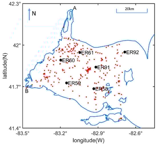
Figure 1.
Map of Lake Erie and data sites. Detail of western basin shoreline showing the Detroit River (A), Maumee River (B), NOAA (red dots), and GLENDA (black dots).
The western basin map was compiled from the Great Lakes Environmental Research Laboratory (GLERL) (Figure 1). The meteorological indicators, including shortwave radiation, cloud cover, air temperature, relative humidity, wind speed, and precipitation, were selected in this study. Solar radiation data were provided by Cleveland Hopkins International Airport, on the south shore of Lake Erie. Precipitation data were obtained from Port Stanley, which is located on the north shore of the central basin of Lake Erie. Cloud cover data were obtained from the Cleveland Burke Lakefront Airport, located on the south shore of the lake. The data were in the form of verbal observations, such as overcast, broken, clear, etc. Each observation was replaced with a corresponding value for the fraction of the sky covered with cloud. Relative humidity data were collected from Erieau and Windsor stations, located on the north shore of the central basin. Wind speed and air temperature data were collected from two sources. Most data were obtained from the National Ocean and Atmospheric Administration’s (NOAA) National Data Buoy Center’s buoy located in the central basin (Station ID: 45005) of Lake Erie and these data were only available during months without ice cover. Data from the Cleveland Burke airport were used for the months with ice cover. For information on the data resources of the Detroit and Maumee Rivers, see Appendix A and Appendix B.
Observed surface water temperature data from 2002 to 2015 were obtained from NOAA. The observed Chl-a concentrations from 2002 to 2015 were retrieved from the Great Lakes Environmental database system (GLENDA), and they were sampled through the water column during spring and in the epilimnion (from 2 to 4 m depths) during summer. The observed bio-volumes () were converted to Chl-a biomass () using the conversion formula: with species-specific values of a and b [36].
2.2. Modeling Methodology
2.2.1. GLM-AED Description
The one-dimensional model GLM-AED (General Lake Model-Aquatic Ecosystem Dynamics module library) is open-source [37], and it has been applied to various water bodies, such as temperate lakes [19] and reservoirs [38]. The advantage of computational requirements makes it a common tool for long-term simulations. The hydrodynamic model GLM assumes there is no horizontal variability and adopts a flexible Lagrangian structure, making it possible to adjust the vertical layer thicknesses dynamically to resolve the water column structure. The module solves the turbulent kinetic energy balance to model the surface heat and momentum budgets. The biogeochemical module AED can simulate nutrients, phytoplankton, and oxygen. In this module, 15 state variables were applied to model Chl-a, including dissolved oxygen (DO), four dissolved inorganic groups (dissolved reactive phosphorus (PO4), nitrate (NO3), ammonium (NH4), and reactive silica [39]), three dissolved organic groups (dissolved organic nitrogen (DON), dissolved organic phosphorus (DOP), and dissolved organic carbon (DOC)), and three particulate detrital organic groups (particulate organic nitrogen (PON), particulate organic phosphorus (POP), and particulate organic carbon (POC)), diatoms (DIAT), chlorophytes (CHLOR), cryptophytes (CRYPT), and cyanobacteria (CYANO). Given the difficulties in simulating the changes in the associated population dynamics, we neglected to model dreissenid mussels and zooplankton, subsuming the related mortality and nutrient cycling into the respiration parameter [40].
GLM-AED was initialized on 1 May 2002. The mean daily meteorological forcing data included air temperature, wind speed, relative humidity, precipitation, shortwave solar radiation, and cloud cover. Mean daily boundary conditions included flow rates and water quality state variables for the Detroit River and Maumee River (flow, temperature, and the water quality state variables). The boundary of outflow was specified as the central basin, and the flow rate was calculated based on water balance from the flow rates of the Detroit River and Maumee River, evaporation, and the observed water levels [41,42]. The model was calibrated to the observed surface water temperature and Chl-a concentrations from 2002 to 2015.
2.2.2. ANN Description
The architecture of an artificial neural network (ANN) is typically composed of the input layer, the hidden layer(s), and the output layer [43]. The nodes in the input layer transmit the information to the nodes in the hidden layer by applying an activation function, each value of each node in the input layer is multiplied by its weight to obtain a new value, and then the new value of each node in the hidden layer is multiplied by its weight and pass to the node in the output layer by applying an activation function to get the final output [44]. The weights are assigned during training the ANN to minimize errors between the outputs and the targets [45]. The architecture of the ANN is shown in Figure 2.
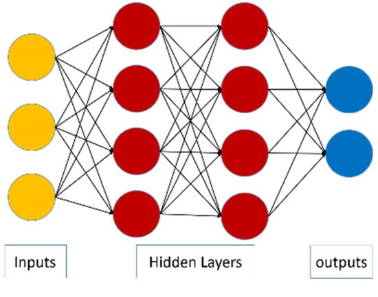
Figure 2.
Schematic view of ANN.
In this study, a multilayer perceptron (MLP) with a backpropagation algorithm was used since it was the most commonly used training methodology [46] and this kind of network has already been widely used for describing non-linear relationships in previous studies [28,29,47]. The inputs in the ANN model were the same as GLM-AED, including meteorological forcing, as well as flow rates, temperature, and 15 state variables of the Detroit and Maumee Rivers, so the number of nodes in the input layer is 40. Particularly, because the salinity of Lake Erie is constant with a value of 0 in GLM-AED, the salinity was not regarded as input in the ANN model. Due to the lack of continuous data for Chl-a concentrations, the simulated Chl-a concentrations from GLM-AED were regarded as the targets during the training process in the ANN model. The number of nodes in the output layer is 1 since there was only one output of Chl-a. The number of nodes in the hidden layers typically satisfies Equation (1) according to the previous study [48]:
where ni, nh, and no represent the number of nodes in the input, hidden, and output layers, respectively. In this study, the number of nodes in the hidden layers was in the range of 14–81. Between the input layer and the hidden layers, as well as the hidden layers and the output layer, the sigmoid activation function was used [49]. The training ranges of the learning rate for weight updates, momentum applied to the weight updates, and batch size representing the preferred number of instances to process were 0.1–0.5, 0.1–0.8, and 10–1000, with steps of 0.1, 0.1, and 5. The database from 2002 to 2015 was divided into two parts, including training and testing sections.
2.2.3. Performance Metrics of the Predictive Tool
RMSE and MAE are commonly applied in model performance evaluation for hydrodynamic and water quality models and statistical models [50,51]. These two performance measures are in the same unit as the model output, and hence, making them easily interpretable for the reader, and they also work well for continuous long-term simulations [50]. In this study, the root mean square error (RMSE) and mean absolute error based on the previous study were used for evaluating model predictive performance [52]:
3. Results and Discussion
3.1. Performance of Predictive Models
The simulations provided by GLM-AED were compared with the observed surface water temperature and Chl-a from 2002 to 2015. The time-series of surface water temperature showed that the model reproduced the annual variations of water temperature, varying between −5 °C in winter and 25 °C in summer (Figure 3). The RMSE and MAE were 2.95 and 2.75 °C, respectively, which were comparable to previous studies with the applications of the one-dimensional model with an RMSE value of 1–6 °C [53] and three-dimensional model with an RMSE value of 1–3 °C [54] to Lake Erie. In Figure 4, both predicted and observed Chl-a peaks occurred in 2011, with high cyanobacteria in summer (optimum temperature of 25 °C) and diatoms in early spring (optimum temperature of 9.8 °C) [55]. The Chl-a RMSE and MAE were 19.61 and 18.23 , respectively. These errors are comparable to previous studies; for example, Trolle et al. (2008) have obtained an RMSE of 10.4–12.76 in Lake Ravn in Denmark with the application of the one-dimensional DYRESM-CAEDYM (Dynamic Reservoir Simulation Model-Computational Aquatic Ecosystem Dynamics Model) [56]. Silva et al. (2014) underestimated about 110 in Río de la Plata with the application of the three-dimensional ELCOM-CAEDYM (Estuary, Lake and Coastal Ocean Model-Computational Aquatic Ecosystem DYnamics Model) [57]. Disparities still occurred between predictions and observations, which may be due to the simplification of the complicated ecological processes; for example, our model GLM-AED assumes there is no horizontal variability (horizontally averaged) [37]. The parameters used in this model during calibration were listed in Appendix C and Appendix D.
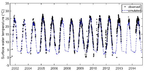
Figure 3.
The simulated and observed surface water temperature comparison at Sta. 45005 (ECCC & NOAA) for 2002–2015.
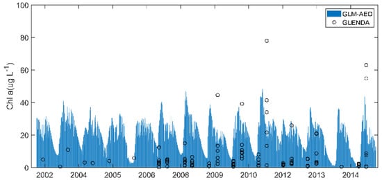
Figure 4.
Comparison between depth-averaged simulations and observed total Chl-a from sampling at GLENDA stations for 2002–2015 (ER 58, 59, 60, 61, 91, 92); The GLENDA data have been converted from biovolume to biomass using the conversions in Reavie et al. (2016).
In the training process of the ANN model, to obtain the smallest errors, the number of the hidden layer was selected as 15. The sigmoid function was used as the activation function between layers. The learning rate, momentum, and batch size were 0.3, 0.2, and 100. With trying different percentages of the database for training, 66% of the total data (2002–2010) and 34% of the total data (2011–2015) were used for training and testing, respectively. Figure 5 showed the scatter density plots for Chl-a concentrations between the predictions from the ANN model (y-axis) and the targets from GLM-AED (x-axis) from 2002 to 2010. The value of R2 was 0.83; thus, compared to the value of approximately 0.73 in the previous study [46], our ANN model can reproduce the target Chl-a concentrations. The RMSE and MAE values during the training process were 3.20 and 2.53 , respectively.
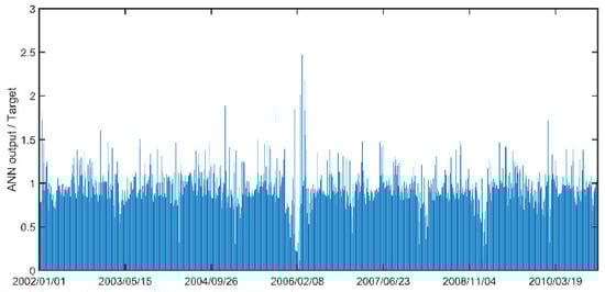
Figure 5.
Performance of ANN in modeling Chl-a concentrations simulated by GLM-AED (Targets) in WLE from 2002 to 2010.
During the testing period, predicted Chl-a concentrations obtained from the ANN model were compared with GLENDA observations from 2011 to 2015, and the RMSE and MAE values were 21.29 and 15.58 , respectively. Compared with the RMSE and MAE values of 23.27 and 19.08 between GLM-AED simulations and GLENDA measurements during 2011 and 2015, the ANN model has a better predictive performance. The predictive performance of ANN and GLM-AED at most stations with RMSE and MAE values in the range of 13.83–21.92 and 9.87–21.49 was better than that at station ER 58 (GLM-AED: RMSE = 60.85, MAE = 41.66; ANN: RMSE = 59.21, MAE = 37.21) and station ER 59 (GLM-AED: RMSE = 48.88, MAE = 32.64; ANN: RMSE = 47.19, MAE = 26.86), which is because stations ER 58 and ER 59 are along the southwest border in the western basin, resulting in the observations at these two stations during summer being larger than the simulations near the Maumee River plume [58], especially in the blooming year 2011 and 2015 [55,59], since one-dimensional GLM-AED represents horizontal homogeneity and the nonlinear relationships in the ANN network prioritizes larger weights for the values with a higher frequency of input database to obtain the minimum statistical errors. Additionally, the computational time of the ANN model was less than two seconds, which was 30 times faster than GLM-AED.
3.2. The Application of ANN to Predict Water Quality under Future Climate Change and Nutrient Management
Making long-term predictions can avoid the effects of short-term variations, such as thermal stratification, heat content, etc. on phytoplankton abundance [60,61], so here, we used the established ANN model to predict future 10-year Chl-a concentrations in WLE from 2021 to 2031.
3.2.1. Future Climate Change and Nutrient Management
For future meteorological data, we downloaded the outputs of CMCC-CM2, one of the CMCC (Euro-Mediterranean Centre on Climate Change)-coupled climate models, which is mainly based on the Community Earth System Model project operated at the National Centre for Atmospheric Research (NCAR) in the USA from CMIP6 (Coupled Model Intercomparison Project) [62]. CMCC-CM2 is the evolution of CMCC-CM [63] applied in CMIP5 [64], and it is composed of the Community Atmosphere Model, the NEMO ocean engine, the Community sea-Ice CodE, and the Community Land Model [65]. The downloaded daily meteorological data included cloud cover, relative humidity, precipitation, shortwave radiation, wind speed, and air temperature, consistent with the inputs in the established ANN and GLM-AED models.
For the Maumee River, the future flow rates (Q) were predicted by rational method, we first calculated base flow (QB) based on the historical flow rates from 2002 to 2015, and then obtained the future flow rates based on the relationship between peak runoff (Q-QB) and precipitation. To achieve a ‘Mild’ bloom for western Lake Erie, reducing the Maumee River’s annual and spring TP loads by 39% and 37% compared to the average loads for 2007–2012 of 2630 and 1275 metric tons [66] was recommended. For dissolved reactive phosphorus (DRP), the Task Force recommended an annual and spring loading reduction of 46% and 41% in the average loads from 2007–2012 of 593 and 256 MT [67]. This corresponds with the understanding that DRP comprised approximately 20% of TP in WLE tributaries with annual and spring DRP targets of 320 and 150 MT (https://legacyfiles.ijc.org/tinymce/uploaded/Draft%20LEEP-Aug29Final.pdf (accessed on 20 August 2013). The POP, DOP, CHLOR, DIAT, CYANO, and CRYPT concentrations were calculated by applying the same formulas described in Appendix B. For the Detroit River, since it is typically under control, the annual P loads are approximately constant with a value of 1080 MT, and the fluctuations in flow rates can be neglected, we used the base flow from 2002 to 2015 as the future flow rates. Additionally, the POP, DOP, CHLOR, DIAT, CYANO, and CRYPT concentrations were calculated by using the same formulas in Appendix A. Since nitrogen and carbon are not critical for CYANO growth, we used the data in 2015 as the future data in these two rivers.
3.2.2. Prediction of Future Water Quality
Under future climate change and nutrient management scenarios, the predicted average annual Chl-a concentrations were in the range of 15–16 . CYANO is the major component of total Chl-a [68], with the optimal temperature for growth above 25 °C [69]. In the future climate scenario, the temperature is 0.27–7.84 °C, which is much lower than the 25 °C that occurred in the summer during 2002 and 2015, so the predicted Chl-a concentrations are lower than the peak values during 2002 and 2015 in Figure 4. Phosphorus is also important for Chl-a growth [70]. In the future nutrient management scenario, phosphorus loads from Detroit and Maumee River are decreased, resulting in lower Chl-a concentrations than those during 2002 and 2015.
Based on the guideline values for recreational utility proposed by the World Health Organization in 2003 [71], shown in Table 1, the moderate-risk category is identified as related >50 of Chl-a. The probability of adverse health effects of future 10-year water quality in WLE would be moderate. To eliminate the adverse health effects, more intense water resource management would be necessary for the future; for example, making more intense phosphorus load reduction strategies for Maumee River than the targets. Additionally, applying agricultural best management practices (BMP) on the Maumee watershed, such as cover crops and filter strips. In our future work, we will predict the water quality of Lake Erie with the application of BMP on the Maumee watershed with the ANN approach. Additionally, we could predict physical features of Lake Erie, such as water temperature, by applying the ANN approach. There are also some limitations in future work, such as the lack of continuous data required for the establishment of ANN.

Table 1.
WHO Recreational Guidance for Chlorophyll a.
4. Conclusions
In this study, the process-based model GLM-AED and the statistical model ANN were established to predict water quality conditions in western Lake Erie. Based on the same inputs as in GLM-AED and the simulated Chl-a concentrations from calibrated GLM-AED during 2002 and 2010, we trained the ANN model, and then we compared the predicted Chl-a concentrations from GLM-AED and ANN with GLENDA observations during 2011 and 2015. The smaller RMSE and MAE values between ANN predictions and observations showed ANN has higher accuracy than GLM-AED. Lastly, the established ANN model was used to predict the future 10-year water quality of WLE, indicating that moderate adverse health effects would occur in the next decade. Particularly, with the lack of inputs from 2016 to 2020, we can still apply trained ANN to predict future water quality conditions, while it is impossible to apply GLM-AED with a lack of continuous input data. Furthermore, the specialized knowledge requirements in the ANN model application are less than the process-based GLM-AED model. Therefore, the ANN model in our study could be a potential tool replacing process-based models for informing long-term future water quality changes in WLE.
Author Contributions
Conceptualization, Q.W. and S.W.; methodology, Q.W. and S.W.; software, Q.W. and S.W.; validation, Q.W. and S.W.; formal analysis, Q.W. and S.W.; investigation, Q.W.; resources, Q.W.; data curation, Q.W.; writing—original draft preparation, Q.W.; writing—review and editing, S.W.; visualization, Q.W.; supervision, S.W.; project administration, S.W.; funding acquisition, S.W. Both authors have read and agreed to the published version of the manuscript.
Funding
This research is partially supported by the Natural Sciences and Engineering Research Council of Canada.
Institutional Review Board Statement
Not applicable.
Informed Consent Statement
Not applicable.
Data Availability Statement
Not applicable.
Conflicts of Interest
The authors declare no conflict of interest.
Appendix A
Table A1.
Summary of Water Quality Data Sources of the Detroit River.
Table A1.
Summary of Water Quality Data Sources of the Detroit River.
| Parameter | Estimated Method |
|---|---|
| Flow | Daily data obtained from Nanette Noorbakhsh (U.S. Army Corps of Engineers) (emails) |
| Temperature | Average of previous three-day air temperature |
| DO | 100% Sat. O2 Conc. = 14.59–0.3955 T + 0.0072 T2–0.0000619 T3 |
| Si | Linear interpolated based on the data obtained from Environmental Monitoring and Reporting Branch_Drinking Water Surveillance Program (emails) |
| NH4 | Linear interpolated based on the data obtained from U.S EPA STORET & Environmental Monitoring and Reporting Branch_Drinking Water Surveillance Program (emails) |
| NO2 & NO3 | Linear interpolated based on the data obtained from U.S EPA STORET & Environmental Monitoring and Reporting Branch_Drinking Water Surveillance Program (emails) |
| PO4 | PO4 = percentage of PO4 (estimated based on Scavia_2014) × TP (TP loading = 1080 MTA/year based on Dolan_2005) |
| PON | Linear interpolated based on the data obtained from U.S EPA STORET & Environmental Monitoring and Reporting Branch_Drinking Water Surveillance Program (emails) |
| DON | Linear interpolated based on the data obtained from U.S EPA STORET & Environmental Monitoring and Reporting Branch_Drinking Water Surveillance Program (emails) |
| POP | POP = 0.6(TP-PO4) |
| DOP | DOP = 0.4(TP-PO4) |
| POC | 0.2 mg L−1 based on 2008 data from Dr. Leon Boegman |
| DOC | Linear interpolated based on the data obtained from Environmental Monitoring and Reporting Branch_Drinking Water Surveillance Program (emails) |
| Chlorophyte | Multiplying the ratio of chlorophyte to TP concentration (Winter_2014) by TP concentration (dividing TP loads by flow rates) |
| Diatom | Multiplying the ratio of diatom to TP concentration (Winter_2014) by TP concentration (dividing TP loads by flow rates) |
| Cyanobacteria | Multiplying the ratio of cyanobacteria to TP concentration (Winter_2014) by TP concentration (dividing TP loads by flow rates) |
| Cryptophyte | Multiplying the ratio of cryptophyte to TP concentration (Winter_2014) by TP concentration (dividing TP loads by flow rates) |
Appendix B
Table A2.
Summary of Water Quality Data Sources of the Maumee River.
Table A2.
Summary of Water Quality Data Sources of the Maumee River.
| Parameter | Estimated Method |
|---|---|
| Flow | Downloaded from Heidelberg college |
| Temperature | Average of previous three-day air temperature |
| DO | 100% Sat. O2 Conc. = 14.59–0.3955 T + 0.0072 T2–0.0000619 T3 |
| Si | SiO2 = 3.2 mg L−1 = 114 mmol/m3 based on 2008 data from Dr. Boegman |
| NH4 | NH4 = 0.08 × TKN (0.08 is obtained based on 2008 data from Dr. Boegman) |
| NO2 & NO3 | Downloaded from Heidelberg college |
| PO4 | Downloaded from Heidelberg college |
| PON | PON = 0.25 × TKN (0.25 is obtained based on 2008 data from Dr. Boegman) |
| DON | PON = 0.25 × TKN (0.25 is obtained based on 2008 data from Dr. Boegman) |
| POP | POP = 0.6(TP-PO4) [TP & PO4 both downloaded from Heidelberg college ] |
| DOP | DOP = 0.4(TP-PO4) [TP & PO4 both downloaded from Heidelberg college ] |
| POC | POC = 0.5 mg L−1 based on 2008 data from Dr. Boegman |
| DOC | DOC = 3 mg L−1 based on 2008 data from Dr. Boegman |
| Chlorophyte | Multiplying the ratios of chlorophyte to TP concentration (different ratio values for different months displayed in Bridgeman_2012) by TP concentration (Heidelberg college) |
| Diatom | Multiplying the ratios of daitom to TP concentration (different ratio values for different months displayed in Bridgeman_2012) by TP concentration (Heidelberg college) |
| Cyanobacteria | Multiplying the ratios of cyanobacteria to TP concentration (different ratio values for different months displayed in Bridgeman_2012) by TP concentration (Heidelberg college) |
| Cryptophyte | Multiplying the ratios of cryptophyte to TP concentration (different ratio values for different months displayed in Bridgeman_2012) by TP concentration (Heidelberg college) |
Appendix C
Table A3.
Adjusted hydrodynamic and chemical parameters in GLM-AED.
Table A3.
Adjusted hydrodynamic and chemical parameters in GLM-AED.
| Parameter | Description | Units | Default Value | Assigned Value |
|---|---|---|---|---|
| Kw | Extinction coefficient for PAR radiation | /m | 0.9 | 0.76 |
| wind_factor | Scaling factor that is used to multiply the wind speed data | – | 1.0 | 0.9 |
| lw_factor | Scaling factor that is used to multiply the longwave data | mmol/m3 | 1.0 | 0.8 |
| cloud_mode | Switch to configure the atmospheric longwave emissivity sub-model | mmol/m2/day | 4 | 1 |
| theta_sed_frp | Temperature multiplier for temperature dependence of sediment phosphate flux | – | 1.08 | 1.1 |
| Fsed_frp | Maximum flux of oxygen across the sediment water interface into the sediment | mmol/m2/day | 0.08 | 0.2 |
Appendix D
Table A4.
Adjusted phytoplankton parameters in AED.
Table A4.
Adjusted phytoplankton parameters in AED.
| Parameter | Description | Unit | CHLOR | DIAT | CYANO | CRYPT | ||||
|---|---|---|---|---|---|---|---|---|---|---|
| Default Value | Assigned Value | Default Value | Assigned Value | Default Value | Assigned Value | Default Value | Assigned Value | |||
| Pmax | Maximum phytoplankton growth rate of 20 °C | 1/d | 1.1 | 1.394 | 1.1 | 2.38 | 1.1 | 1.8 | 1.1 | 1.386 |
| vT | Arrhenius temp scaling coefficient for growth | - | 1.05 | 1.05 | 1.05 | 1.04 | 1.05 | 1.048 | 1.05 | 1.05 |
| Tstd | Standard temperature | °C | 15 | 20 | 15 | 7 | 15 | 21 | 15 | 18 |
| Topt | Optimum temperature | °C | 24 | 24 | 24 | 9.8 | 24 | 25 | 24 | 21 |
| Tmax | Maximum temperature | °C | 35 | 35 | 35 | 18.5 | 35 | 37 | 35 | 29 |
| kr | Phytoplankton respiration/metabolic loss rate of 20 °C | 1/d | 0.07 | 0.031 | 0.07 | 0.035 | 0.07 | 0.04 | 0.07 | 0.0285 |
| vr | Arrhenius temperature scaling for phytoplankton respiration | - | 1.06 | 1.06 | 1.06 | 1.06 | 1.06 | 1.06 | 1.06 | 1.06 |
References
- Huisman, J.; Codd, G.A.; Paerl, H.W.; Ibelings, B.W.; Verspagen, J.M.; Visser, P.M. Cyanobacterial blooms. Nat. Rev. Microbiol. 2018, 16, 471–483. [Google Scholar] [CrossRef]
- Paerl, H.W.; Havens, K.E.; Xu, H.; Zhu, G.; McCarthy, M.J.; Newell, S.E.; Scott, J.T.; Hall, N.S.; Otten, T.G.; Qin, B. Mitigating eutrophication and toxic cyanobacterial blooms in large lakes: The evolution of a dual nutrient (N and P) reduction paradigm. Hydrobiologia 2020, 847, 4359–4375. [Google Scholar] [CrossRef]
- Luo, J.; Li, X.; Ma, R.; Li, F.; Duan, H.; Hu, W.; Qin, B.; Huang, W. Applying remote sensing techniques to monitoring seasonal and interannual changes of aquatic vegetation in Taihu Lake, China. Ecol. Indic. 2016, 60, 503–513. [Google Scholar] [CrossRef]
- Ochumba, P.B.; Kibaara, D.I. Observations on blue-green algal blooms in the open waters of Lake Victoria, Kenya. Afr. J. Ecol. 1989, 27, 23–34. [Google Scholar] [CrossRef]
- Tijdens, M.; Hoogveld, H.L.; Kamst-van Agterveld, M.P.; Simis, S.G.; Baudoux, A.-C.; Laanbroek, H.J.; Gons, H.J. Population dynamics and diversity of viruses, bacteria and phytoplankton in a shallow eutrophic lake. Microb. Ecol. 2008, 56, 29–42. [Google Scholar] [CrossRef] [Green Version]
- Wang, M.; Shi, W.; Tang, J. Water property monitoring and assessment for China’s inland Lake Taihu from MODIS-Aqua measurements. Remote Sens. Environ. 2011, 115, 841–854. [Google Scholar] [CrossRef]
- Bolsenga, S.J.; Herdendorf, C.E. Lake Erie and Lake St. Clair Handbook; Wayne State University Press: Detroit, MI, USA, 1993. [Google Scholar]
- Davis, C.C. Plants in Lakes Erie and Ontario, and changes of their numbers and kinds. Bull. Buffalo Soc. Nat. Sci. 1969, 25, 18–44. [Google Scholar]
- Scavia, D.; Allan, J.D.; Arend, K.K.; Bartell, S.; Beletsky, D.; Bosch, N.S.; Brandt, S.B.; Briland, R.D.; Daloğlu, I.; DePinto, J.V. Assessing and addressing the re-eutrophication of Lake Erie: Central basin hypoxia. J. Great Lakes Res. 2014, 40, 226–246. [Google Scholar] [CrossRef]
- Scavia, D.; DePinto, J.; Auer, M.; Bertani, I.; Bocaniov, S.; Chapra, S.; Leon, L.; McCrimmon, C.; Obenour, D.; Peterson, G. Great Lakes Water Quality Agreement Nutrient Annex Objectives and Targets Task Team Ensemble Multi-Modeling Report; Great Lakes National Program Office, USEPA: Chicago, IL, USA, 2016. [Google Scholar]
- Sweeney, R.A. Dead” Sea of North America?—Lake Erie in the 1960 s and’70 s. J. Great Lakes Res. 1993, 19, 198–199. [Google Scholar] [CrossRef]
- Makarewicz, J.C.; Bertram, P. Evidence for the restoration of the Lake Erie ecosystem. Bioscience 1991, 41, 216–223. [Google Scholar] [CrossRef] [Green Version]
- Makarewicz, J.C. Phytoplankton biomass and species composition in Lake Erie, 1970 to 1987. J. Great Lakes Res. 1993, 19, 258–274. [Google Scholar] [CrossRef]
- Kane, D.D.; Conroy, J.D.; Richards, R.P.; Baker, D.B.; Culver, D.A. Re-eutrophication of Lake Erie: Correlations between tributary nutrient loads and phytoplankton biomass. J. Great Lakes Res. 2014, 40, 496–501. [Google Scholar] [CrossRef]
- Millie, D.F.; Fahnenstiel, G.L.; Bressie, J.D.; Pigg, R.J.; Rediske, R.R.; Klarer, D.M.; Tester, P.A.; Litaker, R.W. Late-summer phytoplankton in western Lake Erie (Laurentian Great Lakes): Bloom distributions, toxicity, and environmental influences. Aquat. Ecol. 2009, 43, 915–934. [Google Scholar] [CrossRef] [Green Version]
- Zhang, H.; Boegman, L.; Scavia, D.; Culver, D.A. Spatial distributions of external and internal phosphorus loads in Lake Erie and their impacts on phytoplankton and water quality. J. Great Lakes Res. 2016, 42, 1212–1227. [Google Scholar] [CrossRef]
- Higgins, S.N.; Malkin, S.Y.; Todd Howell, E.; Guildford, S.J.; Campbell, L.; Hiriart-Baer, V.; Hecky, R.E. An ecological review of Cladophora glomerata (Chlorophyta) in the Laurentian Great Lakes 1. J. Phycol. 2008, 44, 839–854. [Google Scholar] [CrossRef]
- Rousso, B.Z.; Bertone, E.; Stewart, R.; Hamilton, D.P. A systematic literature review of forecasting and predictive models for cyanobacteria blooms in freshwater lakes. Water Res. 2020, 115959. [Google Scholar] [CrossRef] [PubMed]
- Snortheim, C.A.; Hanson, P.C.; McMahon, K.D.; Read, J.S.; Carey, C.C.; Dugan, H.A. Meteorological drivers of hypolimnetic anoxia in a eutrophic, north temperate lake. Ecol. Modell. 2017, 343, 39–53. [Google Scholar] [CrossRef] [Green Version]
- Zhang, H.; Culver, D.A.; Boegman, L. A two-dimensional ecological model of Lake Erie: Application to estimate dreissenid impacts on large lake plankton populations. Ecol. Modell. 2008, 214, 219–241. [Google Scholar] [CrossRef]
- Leon, L.F.; Smith, R.E.; Hipsey, M.R.; Bocaniov, S.A.; Higgins, S.N.; Hecky, R.E.; Antenucci, J.P.; Imberger, J.A.; Guildford, S.J. Application of a 3D hydrodynamic–biological model for seasonal and spatial dynamics of water quality and phytoplankton in Lake Erie. J. Great Lakes Res. 2011, 37, 41–53. [Google Scholar] [CrossRef]
- Zhou, S.; Xu, L.; Hao, L.; Xiao, H.; Yao, Y.; Qi, L.; Yao, Y. A review on low-dimensional physics-based models of systemic arteries: Application to estimation of central aortic pressure. Biomed. Eng. Online 2019, 18, 41. [Google Scholar] [CrossRef] [PubMed] [Green Version]
- Solomatine, D.; See, L.M.; Abrahart, R. Data-driven modelling: Concepts, approaches and experiences. In Practical Hydroinformatics; Springer: Berlin/Heidelberg, Germany, 2009; pp. 17–30. [Google Scholar]
- Solomatine, D.P.; Ostfeld, A. Data-driven modelling: Some past experiences and new approaches. J. Hydroinform. 2008, 10, 3–22. [Google Scholar] [CrossRef] [Green Version]
- Wang, Q.; Wang, S. Machine Learning-Based Water Level Prediction in Lake Erie. Water 2020, 12, 2654. [Google Scholar] [CrossRef]
- Choubin, B.; Malekian, A.; Samadi, S.; Khalighi-Sigaroodi, S.; Sajedi-Hosseini, F. An ensemble forecast of semi-arid rainfall using large-scale climate predictors. Meteorol. Appl. 2017, 24, 376–386. [Google Scholar] [CrossRef] [Green Version]
- Lee, K.Y.; Chung, N.; Hwang, S. Application of an artificial neural network (ANN) model for predicting mosquito abundances in urban areas. Ecol. Inform. 2016, 36, 172–180. [Google Scholar] [CrossRef] [Green Version]
- Gebler, D.; Szoszkiewicz, K.; Pietruczuk, K. Modeling of the river ecological status with macrophytes using artificial neural networks. Limnologica 2017, 65, 46–54. [Google Scholar] [CrossRef]
- Rocha, J.C.; Peres, C.K.; Buzzo, J.L.L.; de Souza, V.; Krause, E.A.; Bispo, P.C.; Frei, F.; Costa, L.S.; Branco, C.C. Modeling the species richness and abundance of lotic macroalgae based on habitat characteristics by artificial neural networks: A potentially useful tool for stream biomonitoring programs. J. Appl. Phycol. 2017, 29, 2145–2153. [Google Scholar] [CrossRef]
- Olaya-Marín, E.J.; Martínez-Capel, F.; Vezza, P. A comparison of artificial neural networks and random forests to predict native fish species richness in Mediterranean rivers. Knowl. Manag. Aquat. Ecosyst. 2013, 409, 07. [Google Scholar] [CrossRef] [Green Version]
- Segurado, P.; Almeida, C.; Neves, R.; Ferreira, M.T.; Branco, P. Understanding multiple stressors in a Mediterranean basin: Combined effects of land use, water scarcity and nutrient enrichment. Sci. Total Environ. 2018, 624, 1221–1233. [Google Scholar] [CrossRef] [PubMed]
- U.S. Environmental Protection Agency. State Development of Numeric Criteria for Nitrogen and Phosphorus Pollution; US Environmental Protection Agency: Washington, DC, USA, 2015.
- Tyson, J.; Davies, D.; Mackey, S. Influence of riverine inflows on western Lake Erie: Implications for fisheries management. In Proceedings of the 12th Biennial Coastal Zone Conference, Cleveland, OH, USA, 15–19 July 2001. [Google Scholar]
- USEPA. Recommended Phosphorus Loading Targets for Lake Erie. Annex 4 Objectives and Targets Task Team Final Report to the Nutrients Annex Subcommittee. 11 May 2015. 2015. Available online: https://www.epa.gov/sites/default/files/2015-06/documents/report-recommended-phosphorus-loading-targets-lake-erie-201505.pdf (accessed on 5 June 2021).
- Matisoff, G.; Kaltenberg, E.M.; Steely, R.L.; Hummel, S.K.; Seo, J.; Gibbons, K.J.; Bridgeman, T.B.; Seo, Y.; Behbahani, M.; James, W.F. Internal loading of phosphorus in western Lake Erie. J. Great Lakes Res. 2016, 42, 775–788. [Google Scholar] [CrossRef]
- Reavie, E.D.; Cai, M.; Twiss, M.R.; Carrick, H.J.; Davis, T.W.; Johengen, T.H.; Gossiaux, D.; Smith, D.E.; Palladino, D.; Burtner, A. Winter–spring diatom production in Lake Erie is an important driver of summer hypoxia. J. Great Lakes Res. 2016, 42, 608–618. [Google Scholar] [CrossRef]
- Hipsey, M.R.; Bruce, L.C.; Boon, C.; Busch, B.; Carey, C.C.; Hamilton, D.P.; Hanson, P.C.; Read, J.S.; De Sousa, E.; Weber, M. A General Lake Model (GLM 3.0) for Linking with High-Frequency Sensor Data from the Global Lake Ecological Observatory Network (GLEON). Geosci. Model Dev. 2019, 12, 473–523. [Google Scholar] [CrossRef] [Green Version]
- Weber, M.; Rinke, K.; Hipsey, M.; Boehrer, B. Optimizing withdrawal from drinking water reservoirs to reduce downstream temperature pollution and reservoir hypoxia. J. Environ. Manag. 2017, 197, 96–105. [Google Scholar] [CrossRef]
- Hodges, B.; Dallimore, C.; Estuary, L.J.C.F.W.R. Coastal Ocean Model: ELCOM Science Manual v2.2; University of Western Australia: Perth, Australia, 2015. [Google Scholar]
- Hipsey, M.; Bruce, L.; Hamilton, D. Aquatic Ecodynamics (AED) Model Library Science Manual; The University of Western Australia Technical Manual: Perth, Australia, 2013; Volume 34. [Google Scholar]
- Gibson, J.; Prowse, T.; Peters, D. Hydroclimatic controls on water balance and water level variability in Great Slave Lake. Hydrol. Process. 2006, 20, 4155–4172. [Google Scholar] [CrossRef]
- Kebede, S.; Travi, Y.; Alemayehu, T.; Marc, V. Water balance of Lake Tana and its sensitivity to fluctuations in rainfall, Blue Nile basin, Ethiopia. J. Hydrol. 2006, 316, 233–247. [Google Scholar] [CrossRef]
- Khalil, B.; Ouarda, T.; St-Hilaire, A. Estimation of water quality characteristics at ungauged sites using artificial neural networks and canonical correlation analysis. J. Hydrol. 2011, 405, 277–287. [Google Scholar] [CrossRef]
- Wu, W.; Dandy, G.C.; Maier, H.R. Protocol for developing ANN models and its application to the assessment of the quality of the ANN model development process in drinking water quality modelling. Environ. Model. Softw. 2014, 54, 108–127. [Google Scholar] [CrossRef]
- Motamarri, S.; Boccelli, D.L. Development of a neural-based forecasting tool to classify recreational water quality using fecal indicator organisms. Water Res. 2012, 46, 4508–4520. [Google Scholar] [CrossRef] [PubMed]
- García-Alba, J.; Bárcena, J.F.; Ugarteburu, C.; García, A. Artificial neural networks as emulators of process-based models to analyse bathing water quality in estuaries. Water Res. 2019, 150, 283–295. [Google Scholar] [CrossRef] [PubMed]
- Park, Y.-S.; Lek, S. Artificial Neural Networks: Multilayer Perceptron for Ecological Modeling. In Developments in Environmental Modelling; Elsevier: Amsterdam, The Netherlands, 2016; Volume 28, pp. 123–140. [Google Scholar]
- Fletcher, D.; Goss, E. Forecasting with neural networks: An application using bankruptcy data. Inf. Manag. 1993, 24, 159–167. [Google Scholar] [CrossRef]
- Jiang, Y.; Nan, Z.; Yang, S. Risk assessment of water quality using Monte Carlo simulation and artificial neural network method. J. Environ. Manag. 2013, 122, 130–136. [Google Scholar] [CrossRef] [PubMed]
- Moriasi, D.N.; Gitau, M.W.; Pai, N.; Daggupati, P. Hydrologic and water quality models: Performance measures and evaluation criteria. Trans. ASABE 2015, 58, 1763–1785. [Google Scholar]
- Jacovides, C.; Kontoyiannis, H. Statistical procedures for the evaluation of evapotranspiration computing models. Agric. Water Manag. 1995, 27, 365–371. [Google Scholar] [CrossRef]
- Zhang, Y.-F.; Fitch, P.; Thorburn, P.J. Predicting the Trend of Dissolved Oxygen Based on the kPCA-RNN Model. Water 2020, 12, 585. [Google Scholar] [CrossRef] [Green Version]
- Boegman, L.; Sleep, S. Feasibility of bubble plume destratification of central Lake Erie. J. Hydraul. Eng. 2012, 138, 985–989. [Google Scholar] [CrossRef]
- Liu, W.; Bocaniov, S.A.; Lamb, K.G.; Smith, R.E. Three dimensional modeling of the effects of changes in meteorological forcing on the thermal structure of Lake Erie. J. Great Lakes Res. 2014, 40, 827–840. [Google Scholar] [CrossRef]
- Michalak, A.M.; Anderson, E.J.; Beletsky, D.; Boland, S.; Bosch, N.S.; Bridgeman, T.B.; Chaffin, J.D.; Cho, K.; Confesor, R.; Daloğlu, I. Record-setting algal bloom in Lake Erie caused by agricultural and meteorological trends consistent with expected future conditions. Proc. Natl. Acad. Sci. USA 2013, 201216006. [Google Scholar] [CrossRef] [PubMed] [Green Version]
- Trolle, D.; Skovgaard, H.; Jeppesen, E. The Water Framework Directive: Setting the phosphorus loading target for a deep lake in Denmark using the 1D lake ecosystem model DYRESM–CAEDYM. Ecol. Modell. 2008, 219, 138–152. [Google Scholar] [CrossRef]
- Silva, C.P.; Marti, C.L.; Imberger, J. Physical and biological controls of algal blooms in the Río de la Plata. Environ. Fluid Mech. 2014, 14, 1199–1228. [Google Scholar] [CrossRef]
- Wynne, T.T.; Stumpf, R.P. Spatial and temporal patterns in the seasonal distribution of toxic cyanobacteria in western Lake Erie from 2002–2014. Toxins 2015, 7, 1649–1663. [Google Scholar] [CrossRef] [Green Version]
- Manning, N.F.; Wang, Y.-C.; Long, C.M.; Bertani, I.; Sayers, M.J.; Bosse, K.R.; Shuchman, R.A.; Scavia, D. Extending the forecast model: Predicting Western Lake Erie harmful algal blooms at multiple spatial scales. J. Great Lakes Res. 2019, 45, 587–595. [Google Scholar] [CrossRef]
- Soranno, P.; Carpenter, S.; Lathrop, R. Internal phosphorus loading in Lake Mendota: Response to external loads and weather. Can. J. Fish. Aquat. Sci. 1997, 54, 1883–1893. [Google Scholar] [CrossRef]
- Tolotti, M.; Thies, H.; Nickus, U.; Psenner, R. Temperature modulated effects of nutrients on phytoplankton changes in a mountain lake. In Phytoplankton Responses to Human Impacts at Different Scales; Springer: Berlin/Heidelberg, Germany, 2012; pp. 61–75. [Google Scholar]
- Eyring, V.; Bony, S.; Meehl, G.A.; Senior, C.A.; Stevens, B.; Stouffer, R.J.; Taylor, K.E. Overview of the Coupled Model Intercomparison Project Phase 6 (CMIP6) experimental design and organization. Geosci. Model Dev. 2016, 9, 1937–1958. [Google Scholar] [CrossRef] [Green Version]
- Scoccimarro, E.; Gualdi, S.; Bellucci, A.; Sanna, A.; Giuseppe Fogli, P.; Manzini, E.; Vichi, M.; Oddo, P.; Navarra, A. Effects of tropical cyclones on ocean heat transport in a high-resolution coupled general circulation model. J. Clim. 2011, 24, 4368–4384. [Google Scholar] [CrossRef] [Green Version]
- Taylor, K.E.; Stouffer, R.J.; Meehl, G.A. An overview of CMIP5 and the experiment design. Bull. Am. Meteorol. Soc. 2012, 93, 485–498. [Google Scholar] [CrossRef] [Green Version]
- Cherchi, A.; Fogli, P.G.; Lovato, T.; Peano, D.; Iovino, D.; Gualdi, S.; Masina, S.; Scoccimarro, E.; Materia, S.; Bellucci, A. Global Mean Climate and Main Patterns of Variability in the CMCC-CM2 Coupled Model. Adv. Model. Earth Syst. 2019, 11, 185–209. [Google Scholar] [CrossRef] [Green Version]
- Imteaz, M.A.; Shanableh, A.; Asaeda, T. Technology. Modelling multi-species algal bloom in a lake and inter-algal competitions. Water Sci. 2009, 60, 2599–2611. [Google Scholar] [CrossRef]
- IJC. Ohio Lake Erie Phosphorus Task Force II Final Report; The Commission: New York, NY, USA, 2013. [Google Scholar]
- Barnard, M.A.; Chaffin, J.D.; Plaas, H.E.; Boyer, G.L.; Wei, B.; Wilhelm, S.W.; Rossignol, K.L.; Braddy, J.S.; Bullerjahn, G.S.; Bridgeman, T.B. Roles of Nutrient Limitation on Western Lake Erie CyanoHAB Toxin Production. Toxins 2021, 13, 47. [Google Scholar] [CrossRef] [PubMed]
- Paerl, H.W.; Huisman, J. Blooms like it hot. Science 2008, 320, 57–58. [Google Scholar] [CrossRef] [PubMed] [Green Version]
- Davis, T.W.; Berry, D.L.; Boyer, G.L.; Gobler, C.J. The effects of temperature and nutrients on the growth and dynamics of toxic and non-toxic strains of Microcystis during cyanobacteria blooms. Harmful Algae 2009, 8, 715–725. [Google Scholar] [CrossRef]
- U.S. Environmental Protection Agency. Human Health Recreational Ambient Water Quality Criteria or Swimming Advisories for Microcystins and Cylindrospermopsin (Draft); Office of Water, US Environmental Protection Agency: Washington, DC, USA, 2016.
Publisher’s Note: MDPI stays neutral with regard to jurisdictional claims in published maps and institutional affiliations. |
© 2021 by the authors. Licensee MDPI, Basel, Switzerland. This article is an open access article distributed under the terms and conditions of the Creative Commons Attribution (CC BY) license (https://creativecommons.org/licenses/by/4.0/).