Development of Sensing Algorithms for Object Tracking and Predictive Safety Evaluation of Autonomous Excavators

Abstract

This article presents the sensing and safety algorithms for autonomous excavators operating on construction sites. Safety is a key concern for autonomous construction to reduce collisions and machinery damage. Taking this point into consideration, our study deals with LiDAR data processing that allows for object detection, motion tracking/prediction, and track management, as well as safety evaluation in terms of potential collision risk. In the safety algorithm developed in this study, potential collision risks can be evaluated based on information from excavator working areas, predicted states of detected objects, and calculated safety indices. Experiments were performed using a modified mini hydraulic excavator with Velodyne VLP-16 LiDAR. Experimental validations prove that the developed algorithms are capable of tracking objects, predicting their future states, and assessing the degree of collision risks with respect to distance and time. Hence, the proposed algorithms can be applied to diverse autonomous machines for safety enhancement.

1. Introduction

Excavation is a major task that is performed in the construction sector. It is the process of earthmoving, such as creating building foundations, land grading, pile driving, highway maintenance, etc. Therefore, excavators are considered essential equipment for any construction. With the increasing number of fatal accidents on construction sites, researchers have conducted numerous studies to raise the issue of safety concerns. The construction sites for excavation are dynamic as they include interactions between different objects such as machines and workers, which can increase the chance of potential collisions due to poor visibility, blind spots, and operator carelessness. Thus, there has been a need for more efficient and advanced safety management to tackle such high-risk accidents.

To fully achieve autonomous operations, advanced safety systems are required to protect the workers and construction infrastructure by gathering information from machine dynamics (proprioceptive) and the external environment (exteroceptive) [1]. Various safety management systems have been proposed for construction equipment to detect dangerous proximities, alert operators and workers about these, and identify blind spots by using sensing data obtained from RF (radio frequency) ID techniques, GPS (global positioning system), cameras, and laser scanners [2].

During the past decade, RFID (radio frequency identification) has been the most widely used sensor for safety management, followed by wireless, camera-based, and UWB (ultra-wide-band) sensors [3]. The RTLS (real-time location system) developed by Lee et al. [4], was intended to enhance worker safety using RFID tags. The implementation of this method requires tags to be linked with the target objects and the leaving-out of objects without tags. However, the study lacks in providing a strategy to prevent collisions. Another RFID-based method was proposed by [5] that utilizes RFID tags for identifying and tracking material locations on construction sites. This approach allows for automatic reading of tags by a supervisor. However, the reader requires a specific range of optimal speed to move to achieve higher accuracy. Besides, it requires the installation of multiple labels and receivers, limiting its practicality.

A computer vision-based methodology was proposed by Seo et al. [6] for construction safety and health monitoring. However, the study lacks in determining unsafe conditions and acts for construction sites. At the same time, magnetic-field proximity detection and alarming techniques were proposed by Teizer [7]. Since their experiments were carried out under limited test conditions (i.e., a flat and unobstructed outdoor surface only with one type of vehicle (loader)), further testing is required to apply the developed safety system in the construction sector.

Neito et al. [8] developed a safety system for preventing collisions between workers and machines based on an integration of wireless networks, GPS, and 3D graphics. However, the GPS can lose its accuracy in small and indoor places. Ref. [9] developed the motion capture and recognition framework for safety management, which helps in achieving behavior-based monitoring for unsafe actions. In this study, the framework can collect site videos and motion templates, extract a 3D skeleton from the videos, and detect unsafe actions using skeleton and motion templates. 3D sensing devices such as stereo-vision and depth cameras have been widely utilized to provide distance information from the given 3D spatial information. However, these sensing devices have a limited detection range and sensitivity to lighting, and thus they are not ideally suited for construction safety management.

Kim et al. [10] considered the swing velocity and braking time of swing motion to propose collision avoidance algorithms. A wearable device using augmented reality was proposed by [11] to identify the hazard’s orientation and distance to workers. Since the alarms are based on the worker’s vision, hazards out of the view may not be detected.

An object detection algorithm using a VLP-16 LiDAR was developed by Alireza et al. [12], which used the voxel-based plane algorithm. The pedestrian detection approach was presented by [13] through analyzing the temporal changes of grids in an occupancy map. However, variations of the size of the detected object size in the map may influence the performance of the tracking filter negatively. Although the study has the above limitation and the considered application is not construction equipment, it provides a useful reference in tracking pedestrians that can be equivalent to workers around construction machines.

Fuerstenberg [14] proposed a laser scanner-based method to detect and track pedestrians. The limitation of this methodology is that its classification criteria do not cover all the objects and may not be suitable for tracking vehicles or cyclists. The method of utilizing video frames was proposed by [15] to detect workers and mobile machines, including construction equipment, and to predict their motions by applying a Kalman filter. The limitation of this study is that the proposed tracking filter works with linear states only. A multi-object tracking and management system was proposed in [16], which integrates the unscented Kalman filter (UKF) with joint probabilistic data association (JPDA) and the interacting multiple model filter (IMM). A safety system that can generate warnings to avoid collisions in the excavator was presented by [17], using 2D laser scanners and new safety indices. However, the use of 2D laser scanners restricts the vertical position of the detected objects. Another restriction of this method is that this type of laser scanner allows 270 degree-FOV (field-of-view) and hence, two scanners are needed to meet the full coverage of 360 degrees. The fusion of two laser scanners makes the system expensive and complicated due to the integration of their data.

The majority of prior studies in the area of safety management focused on proximity-detection and utilization of current states of the detected objects that may not be comprehensive in capturing potential safety risks. For example, the proximity between construction equipment and workers may not be used to indicate potential unsafe conditions if a manipulator or vehicle remains stationary (i.e., does not move) or moves rapidly despite sufficient safe margins. Therefore, quantitative and predictive metrics are highly necessary to assess unsafe conditions and potential risks in fully automated excavators.

To tackle the above issue, this study proposes 3D Lidar-based safety algorithms for autonomous excavators that can effectively detect, track, and predict object motion around the excavator, and then evaluate the severity of collision risks using the defined risk metric.

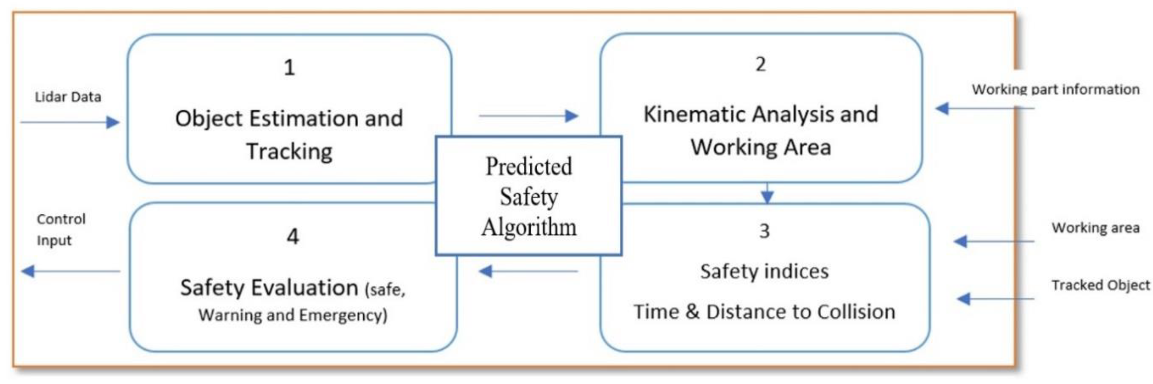
Section 1 describes the introduction and literature review of state-of-the-art methodologies. Section 2 briefly explains a framework of the proposed methodologies that covers object tracking and safety evaluation. Section 3 presents the sensory data processing and safety index calculations. Section 4 provides experimental results and analysis, and the paper is concluded in Section 5.

2. Framework of Object Tracking and Safety Evaluation

The primary goal of this research is to develop a safety module with 3D Lidar to evaluate the severity of potential risks for an autonomous excavator with respect to time and distance by predicting the motions of the detected objects. Figure 1 presents the framework of this study to achieve our objectives. The framework comprises four components that include object detection and tracking (C1), calculation of excavation working area through kinematic analysis (C2), calculation of potential collision severity with respect to time and distance (C3), and safety evaluation (C4).

The first component deals with the estimation and tracking of object positions and velocities through adopting the IMM (interacting multiple model) coupled with a UKF (unscented Kalman filter) and JPDA (joint probabilistic data association). This algorithm facilitates object tracking in a robust manner and the track management can automatically assign track IDs to each detected object [16]. The reason why the IMM-UKF-JPDA approach was selected was to handle the various motion models of different moving objects along with non-linear states. The second part of this work is to calculate the actual and predicted working areas of a modified mini hydraulic excavator by applying a kinematic analysis. Using the position states of the detected objects and working areas and applying the defined safety indices, the time and distance to a collision are estimated as the next step.

Lastly, the collision risks at the current moment were categorized into safe, warning, and emergency based on the computed safety index values. The aforementioned algorithms were developed in the MATLAB environment. Detailed explanations on each step are provided in the following section.

3. Data Processing and Kinematic Analysis

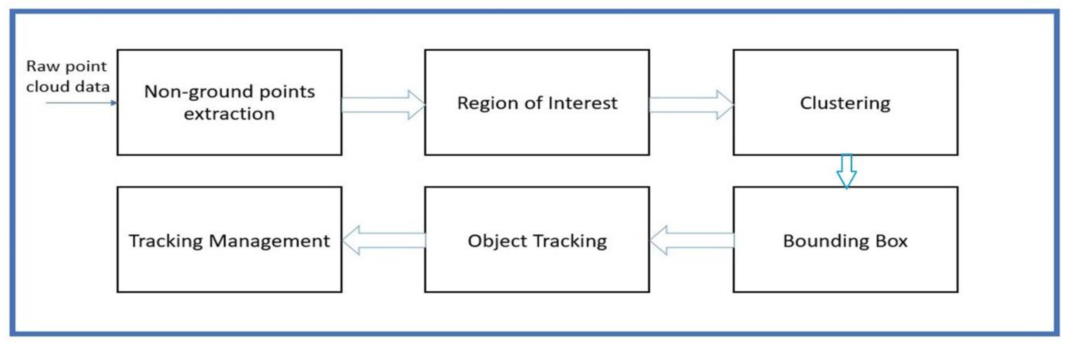
The extraction and processing of sensor data are described in this section, as shown in Figure 2. The VLP-16 LiDAR [18] (VLP-16, Velodyne Lidar, San Jose, CA, US, 2020) was selected as the sensor used for this research as it provides a horizontal detection range of 360 degrees and a vertical range of 30 degrees, respectively. It also generates approximately 300,000 points per second, which allows for fast and high-resolution detection. In addition, the point cloud of each Lidar includes the information of the x, y, and z coordinates that can be used to identify the position of the detected objects. In the study, MATLAB (R2020a, MathWorks, Natick, MA, US, 2020) software was used to store, process, and visualize the point cloud data. The data processing for object tracking and track management was taken through the steps discussed below.

3.1. Extraction of Ground Point Cloud

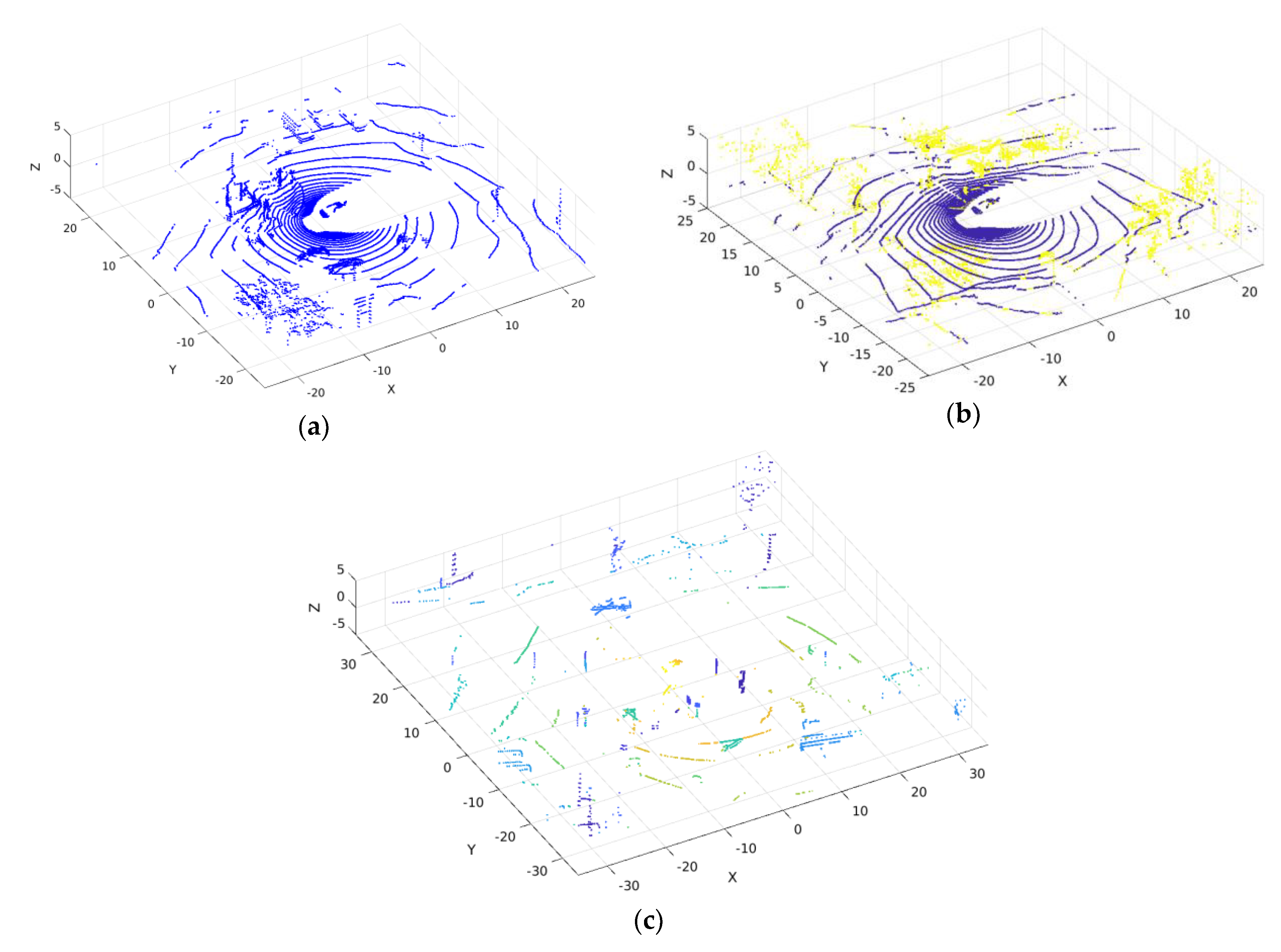
The raw point cloud data represents many points containing ground and non-ground points (Figure 3a). Since our focus is on the detection of moving objects around the excavator, the point clouds representing a ground place (earth surface) firstly need to be eliminated from the point cloud. This is because the moving objects belong to the non-ground points and the ground plane can act as unwanted points during the object detection. Therefore, the extraction of these unwanted points is an essential step, and it can also help reduce the computation load by removing them from the large quantity of unprocessed raw data of LiDAR measurements.

In this research, the point cloud data representing the ground plane were extracted by adopting the MSAC (M-estimator sample and consensus) algorithm as a variant of RANSAC (random sample consensus) [19]. This is a repetitive method to estimate a model from a given dataset containing outliers. To extract the ground points, a plane model was fitted to the raw points cloud by the MSAC algorithm. The RANSAC algorithm can determine the number of outliers by selecting a subset of data and fitting a model to it.

The point clouds representing non-ground points are shown in Figure 3b. After detecting the non-ground points, the next step was to cluster the non-ground points and detect the obstacles (Figure 3c), which is discussed in the next section.

3.2. Obstacle Points

After the removal of non-ground points, the remaining point clouds were formed into clusters. However, these forming clusters are still computationally high, as the LiDAR has a long detection range, thus a region of interest (ROI) was restricted by the defined radius to solve this problem. The point cloud points inside the ROI were considered obstacle points [20]. Clustering was carried out with the obstacle points.

3.3. Clustering and Object Detection

The Euclidean distance required for the clustering process was set to 0.4 m (minimum) ~2 m (maximum) that correspond to the averages of a human (worker) chest width and vehicle size, respectively. Then, the only objects detected within this range were considered for clustering. In this way, the objects that are smaller than a human and bigger than a vehicle were ignored. As the next step, a bounding box was assigned to fit into a single cluster that indicates a detected object. The bounding box generates the center point of each detected object in terms of x, y, and z coordinates. This center point was used for a tracking filter to estimate and predict the object states.

3.4. Object Tracking and Management

To track multiple objects around the excavator, we integrated several filters to design our tracking filter composed of IMM (interacting-multiple-model), UKF (unscented Kalman filter), and JPDA (joint probabilistic data association filter) techniques. The reason for choosing the integrated filters was to handle multiple models representing different motion behaviors (IMM), estimate their non-linear states (UKF), and provide a tracking management system that allows for multitarget tracking in clutter at the stage of the data association (JPDA). The IMM-UKF-JPDA approach is computationally effective for recursive state estimation and the mode probabilities of targets. For the implementation of this filter, we consider model set $\mathbb{M}={\left\{M_j\right\}}_{j=1}^r$ with r = 2 meaning that the M₁, constant velocity (CV), and M₂, constant turn (CT) models are considered. These two models share a common state vector $x={\left[p_x,v_x,p_y,v_y,p_z,v_z,\theta ,\omega ,l,w,h\right]}^T$ consisting of bounding box center points in the $x,y,\mathrm{and}z$ directions $\left(p_x,p_y,and{p}_z\right),$ their corresponding velocities ($v_x,v_y,and{v}_z$), and the yaw angle $\left(\theta \right)$, turn rate ($\omega ),$ and the length ($l)$, width ($w)$, and height ($h)$ of a bounding box. The discrete time–state equation for the CV model is given as:

$$x_{k+1}=\left[\begin{array}{c}{p}_{x,k}+v_{x,k}Tsin{\theta }_k\\ v_{x,k}\\ p_{y,k}+v_{y,k}Tcos{\theta }_k\\ v_{y,k}\\ p_{z,k}\\ v_{z,k}\\ {\theta }_k\\ 0\\ l_k\\ w_k\\ h_k\end{array}\right]+u_k+W_{1,k}.$$

(1)

and the state for the CT model is:

$$x_{k+1}=\left[\begin{array}{c}{p}_{x,k}+\frac{v_{x,k}}{{\omega }_k}(cos{\theta }_k-cos({\omega }_{k}T+{\theta }_k))\\ v_{x,k}\\ p_{y,k}+\frac{v_{y,k}}{{\omega }_k}(sin({\omega }_{k}T+{\theta }_k)-sin{\theta }_k)\\ v_{y,k}\\ p_{z,k}\\ v_{z,k}\\ {\theta }_k+T{\omega }_k\\ {\omega }_k\\ l_k\\ w_k\\ h_k\end{array}\right]+u_k+W_{2,k}.$$

(2)

where $T$ is the sampling time, u_k is the control input of the excavator, and both models include a white Gaussian noise $W_{1,k},\mathrm{and}{W}_{2,k}$ having a mean at zero and the covariance matrices $Q_{1,k}\mathrm{and}{Q}_{2,k}$, respectively. Such models are common for maneuvering multi-object tracking and are extensions of the models found in [21]. Among the two models, the common measurement model is given as:

$$z_k=\left[\begin{array}{l}10000000000\\ 00000000000\\ 00100000000\\ 00000000000\\ 00001000000\\ 00000000000\\ 00000000000\\ 00000000000\\ 00000000000\\ 00000000000\\ 00000000000\end{array}\right]x_k+V_k.$$

(3)

with the measurement noise $V_k$ having the covariance matrix $R_k$.

The next step is to estimate the probability to identify the measurements according to the CV and CT models. The progress of the system among the models is operated on the Markovian model transition probability matrix.

$$\mathsf{\Pi }=\left(\begin{array}{ccc}{p}_{11}& \cdots & p_{r1}\\ ⋮& \ddots & ⋮\\ p_{1r}& \cdots & p_{rr}\end{array}\right)ϵ{ℝ}^{r\times r}.$$

(4)

where $p_{i,j}$ represents the probability of mode transition. Several studies have addressed the integration of the above filter, but this paper follows the five-step process introduced in [21,22]. These steps include (1) interaction, (2) state prediction and measurement validation, (3) data association and tracking management, (4) mode probability update, and (5) combination. Each step can be explained in mathematical representations as follows.

3.4.1. Interaction

In the interaction step, the initial state and covariance of the model filter are probabilistically mixed with the state and covariance of the previous time step.

$$\begin{gathered} {\widehat{x}}_{j,k-1}^{*}={\displaystyle \sum }_{i=1}^r{\mu }_{\left(i|j\right),k-1}{\widehat{x}}_{j,k-1}, \\ {\widehat{P}}_{j,k-1}^{*}={\displaystyle \sum }_{i=1}^r{\mu }_{\left(i|j\right),k-1}[P_{j,k-1}+\left({\widehat{x}}_{j,k-1}-{\widehat{x}}_{j,k-1}^{*}\right){\left({\widehat{x}}_{j,k-1}-{\widehat{x}}_{j,k-1}^{*}\right)}^T]. \end{gathered}$$

(5)

The conditional mode probabilities denoted by ${\mu }_{\left(i|j\right),k-1}$ indicate that the system’s transition from mode i (previous time step) to mode j (current time step), and can be calculated as:

$${\mu }_{\left(i|j\right),k-1}=\frac{P_{ij}{\mu }_{i,k-1}}{{{\displaystyle \sum }}_{i=1}^r{\overline{\mu }}_{i,k-1}}.$$

(6)

The conditional mode probabilities are dependent on the priori mode probabilities of the current frame denoted by ${\mu }_k^{-}$= ${\left({\mu }_{1,k}^{-},\dots ,{\mu }_{r,k}^{-}\right)}^T.$ As seen in Equation (6), the conditional mode probabilities of the current frame can be expressed using the prediction previous frame’s probabilities, and elements of the matrix from Equation (4).

3.4.2. State Prediction and Measurement Validation

The next step is to predict the current states using the stochastic non-linear model. To deal with nonlinearities, UKF is implemented to predict the states and covariances.

$$\begin{gathered} {\mathcal{X}}_{k-1}=[{\widehat{x}}_{k-1}^{\star }\gamma \sqrt{P_{k-1}^{\star }}\oplus {\widehat{x}}_{k-1}^{\star }-\gamma \sqrt{P_{k-1}^{\star }}\oplus {\widehat{x}}_{k-1}^{\star }], \\ {\mathcal{X}}_{i,k}^{\star }=f\left({\mathcal{X}}_{i,k-1},u_{k-1}\right),i=0,\dots ,2n, \end{gathered}$$

(7)

$$\begin{gathered} {\widehat{x}}_k^{-}={\displaystyle \sum }_{i=0}^{2n}{w}_i^m{\mathcal{X}}_{i,k}^{\star }. \\ {P}_k^{-}={\displaystyle \sum }_{i=0}^{2n}{w}_i^c\left({\mathcal{X}}_{i,k}^{\star }-{\widehat{x}}_k^{-}\right){\left({\mathcal{X}}_{i,k}^{\star }-{\widehat{x}}_k^{-}\right)}^T+Q_{k-1}, \\ {\mathcal{X}}_k=[{\widehat{x}}_k^{-}\gamma \sqrt{P_k^{-}}\oplus {\widehat{x}}_k^{-}-\gamma \sqrt{P_k^{-}}\oplus {\widehat{x}}_k^{-}], \\ {\mathcal{K}}_{i,k}=h\left({\mathcal{X}}_{i,k},u_k\right),i=0,\dots ,2n, \\ {\widehat{z}}_k^{-}={\displaystyle \sum }_{i=0}^{2n}{w}_i^m{\mathcal{K}}_{i,k} \end{gathered}$$

(8)

$$S_k={\displaystyle \sum }_{i=0}^{2n}{w}_i^c\left({\mathcal{K}}_{i,k}-{\widehat{z}}_k^{-}\right){\left({\mathcal{K}}_{i,k}-{\widehat{z}}_k^{-}\right)}^T+R_k.$$

(9)

Sigma points, ${\mathcal{X}}_i$ with $i=0,\dots ,2n$ are selected with a square root decomposition of the mixed initial covariance of each filter. Each sigma point has scalar weights $w_i^m$ and $w_i^c$ that are associated, and can be calculated as:

$$w_0^m=\frac{\lambda }{n+1},w_0^c=\frac{\lambda }{n+1}+\left(1-{\alpha }_U^2+{\beta }_U\right).$$

(10)

$$w_i^m=w_i^c=\frac{\lambda }{2\left(n+\lambda \right)},i=1,\dots ,2n,\lambda ={\alpha }_U^2\left(n+{\kappa }_U\right)-n.$$

(11)

$$\gamma =\sqrt{n+\lambda }.$$

(12)

where ${\alpha }_U^{},{\beta }_U,\lambda$, and $\gamma$ are the scalar parameters. The sigma points are propagated with the system function, f. As seen in Equation (7), the sigma points are propagated using the transition function f, and the weighted sigma points are used to calculate the predicted state (${\widehat{x}}_k^{-}$) and covariance ($P_k^{-}$). Similarly, the sigma points are projected by the observation function h in Equation (8) and then the weighted sigma points are involved in generating the predicted measurement (${\widehat{z}}_k^{-}$) and predicted measurement covariance ($S_k$).

A measurement is regarded valid if it falls within the following elliptical validation gate $\mathcal{G}\left({\gamma }_G\right)$. The validation gate of an object $q$ is the same for all the models in $\mathbb{M}$.

$$\begin{array}{c}\mathcal{G}\left({\gamma }_G\right)=\left\{y_k=z_k:{\left(z_k-{\widehat{z}}_{i_q,k}^{-}\right)}^T{S}_{i_{q}k}^{-1}\left(z_k-{\widehat{z}}_{i_q,k}^{-}\right)\le {\gamma }_G\right\}\\ i_q:=\mathrm{argma}{x}_{i\in ℳ}\det \left(S_k^i\right)\end{array}$$

(13)

where $i_q$ is the index of the model in $\mathbb{M}$, ${\gamma }_G$ is the gate threshold, and $y_k$ is the set of validated measurements.

3.4.3. Tracking Management and Data Association

Data association is the step of labeling each detected object with a unique ID and associating the tracking information obtained from a LiDAR sensor that includes the estimation/prediction of the detected object’s position/velocity, with each label. The data association in the tracking filter was dealt with through JPDA [23], which follows the procedure of initialization, confirmation, correction, prediction, and deletion of tracks. Among various data association algorithms, JPDA enables the calculation of all possible target association probability of each observation (see Equations (14)–(17)).

The ‘tentative’ label was given to a newly detected track through the data association process; it was labeled as ‘confirmed’ if a specific track was sufficiently detected to record; the identical ID was assigned if the same track as the current one was detected. The logic flow [24] of JPDA starts with the division of detections from multiple sensors into multiple groups (however, a single LiDAR was used in this study). For each sensor, the distances from detections to existing tracks and a validation matrix were calculated by turns. After the calculation of the validation matrix, tracks and detections were separated into clusters.

The following steps outline how to update each cluster:

• S1: Generation of feasible joint events.
• S2: Calculation of the posteriori probability of each joint event.
• S3: Calculation of the marginal probability of each detection–track pair.
• S4: Reporting of weak detections that are within the validation gate of at least one track.
• S5: Unassigned and weak detections get new tracks.
• S6: Tracks are deleted based on the defined number of scans without detection.
• S7: All tracks are predicted to the latest time value.

To formulate JPDA, we assume to have $x_t^1,\dots ,x_t^N$ and $z_t^1,\dots ,z_t^M$ as the states of $N$ objects and $M$ measurements at time $t$, respectively. Here, the state vector $x_t^j$ means the position and velocity for the $j^{th}$ detected object and the measurements are the cluttered and noisy detected positions observed by a sensor.

The probability of the data association, $p_t\left(d_i^j\right)$ which represents the measurement index i ϵ[M]₀ ≜ {0, 1, …, M}, is defined as follows [24].

$$p_t\left(d_i^j\right)\propto \{\begin{array}{c}\left(1-p_D\right)\beta \mathrm{if}i=0\\ p_D·Ɲ\left(z_t^i;{\widehat{x}}_t^j,{\sum }_S\right)\mathrm{otherwise}.\end{array}$$

(14)

where $p_D$ denotes the detection probability, $\beta$ represents the density of the false detection, ${\widehat{x}}_t^j$ is the prediction state of the object, ${\sum }_S$ is the innovation covariance matrix of the Kalman filter, and $Ɲ$ is the normal distribution. $p_t\left(d_i^j\right)$ is assumed to be a linear Gaussian model and its 0 value means missed or dummy detection.

The joint data association space, Θ, defined in Equation (15) comprises all possible combinations of measurement-to-object assignments in order that each measurement is assigned to at most one object (A1) and each object is uniquely assigned to a measurement (A2).

$$\begin{gathered} \mathsf{\Theta }=\{\theta ={\left(d_i^j\right)}_{i\in {\left[M\right]}_0,j\in \left[\mathrm{N}\right\}}|d_i^j\in \left\{0,1\right\} \\ \wedge {\displaystyle \sum }_{j=1}^N{d}_i^j\le 1,{\forall }_i\in \left[M\right]\mathrm{for}A1 \\ \wedge {{\displaystyle \sum }}_{j=0}^M{d}_i^j=1,{\forall }_j\in \left[N\right]\mathrm{for}A2\}. \end{gathered}$$

(15)

where $\left|\mathsf{\Theta }\right|=:n_h$ is the total number of joint assignments and $\theta$ represents the binary vector that is one possible solution to the data association problem. $\theta \in \mathsf{\Theta }\subseteq {\mathrm{B}}^{N\times \left(M+1\right)}$.

Then, the marginalized JPDA probability, $q_t\left(d_i^j\right)$ over $\mathsf{\Theta }$ can be calculated as

$$q_t\left(d_i^j\right)={\displaystyle \sum }_{\theta \in {\mathsf{\Theta }}_i^j}p\left(\theta \right).$$

(16)

where

$$p\left(\theta \right)={\displaystyle \prod }_{\begin{array}{c}{\forall }_r\in {\left[M\right]}_0\\ {\forall }_k\in \left[N\right]\end{array}}{\left(p_t\left(d_r^k\right)\right)}^{d_r^k}.$$

(17)

As the last step, the normalized $q_t\left(d_i^j\right)$ is used to update the state of the $j^{th}$ detected object.

3.4.4. Mode Probability Update

The mode probabilities are updated in this step using the best-fitting measurements and the uniform mixture model likelihoods ${\lambda }_{j,k}.$

$${\mu }_{q,k}=\frac{{\mu }_{q,k}^{-}{\lambda }_{q,k}}{{\sum }_{i=1}^r{\mu }_{i,k}^{-}{\lambda }_{i,k}}.$$

(18)

where ${\lambda }_{q,k}\stackrel{\mathrm{asm}}{\cong }\mathcal{N}\left({\tilde{z}}_{q,k};0,S_{q,k}\right)$

3.4.5. Combination

In the last step, the updated states of each filter are used to generate the final states and covariances using the model probabilities of tracks as follows.

$${\hat{x}}_{(q,k)}={\displaystyle \sum _i^{}{x}_{i,q,k}{\mu }_{i,q,k}}$$

(19)

$$P_{(q,k)}={\displaystyle \sum _i^{}[P_{i,q,k}+({\hat{x}}_{q,k}-x_{i,q,k}){({\hat{x}}_{q,k}-x_{i,q,k})}^T]{\mu }_{i,q,k}}$$

(20)

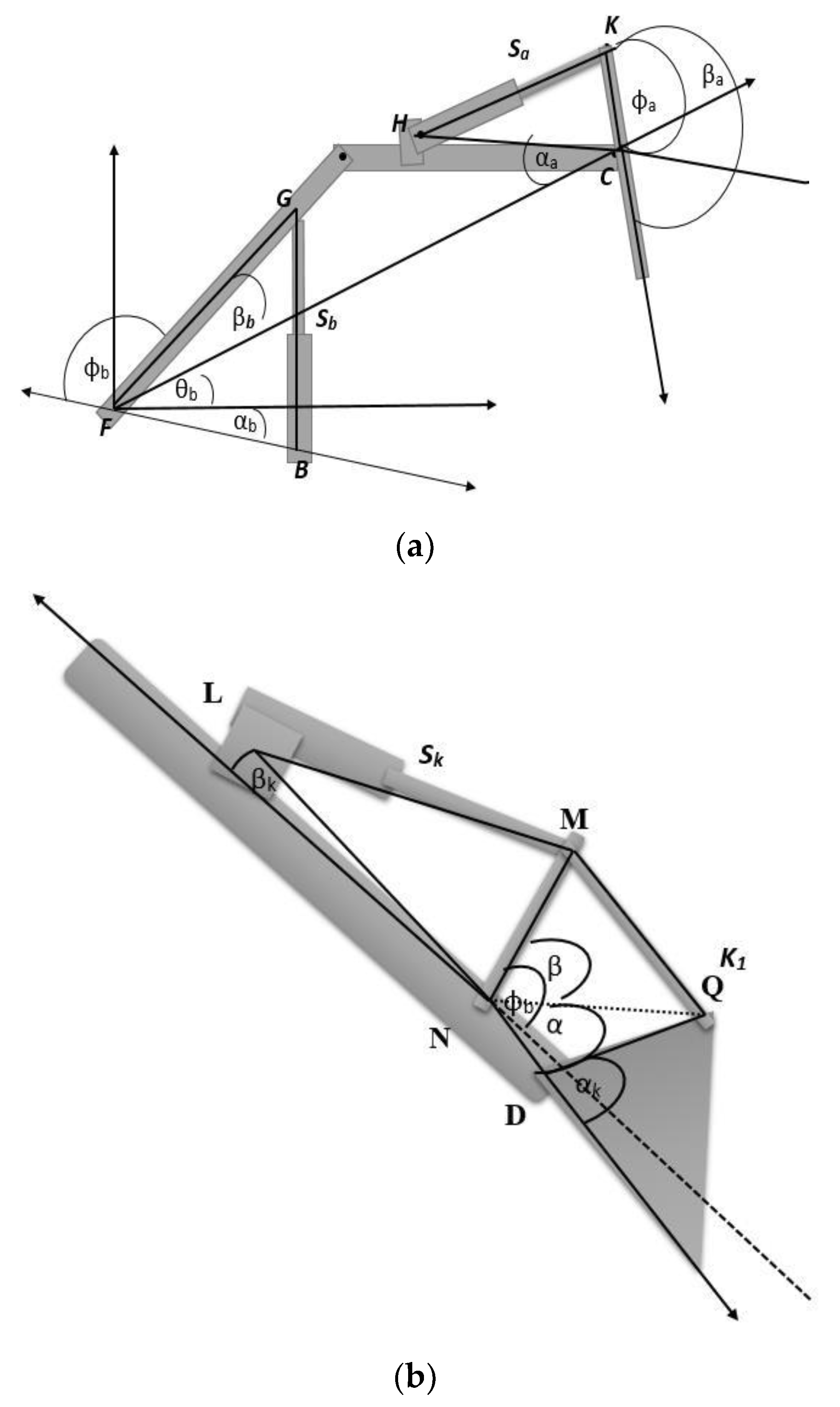
3.5. Calculation of the Excavator’s Working Area

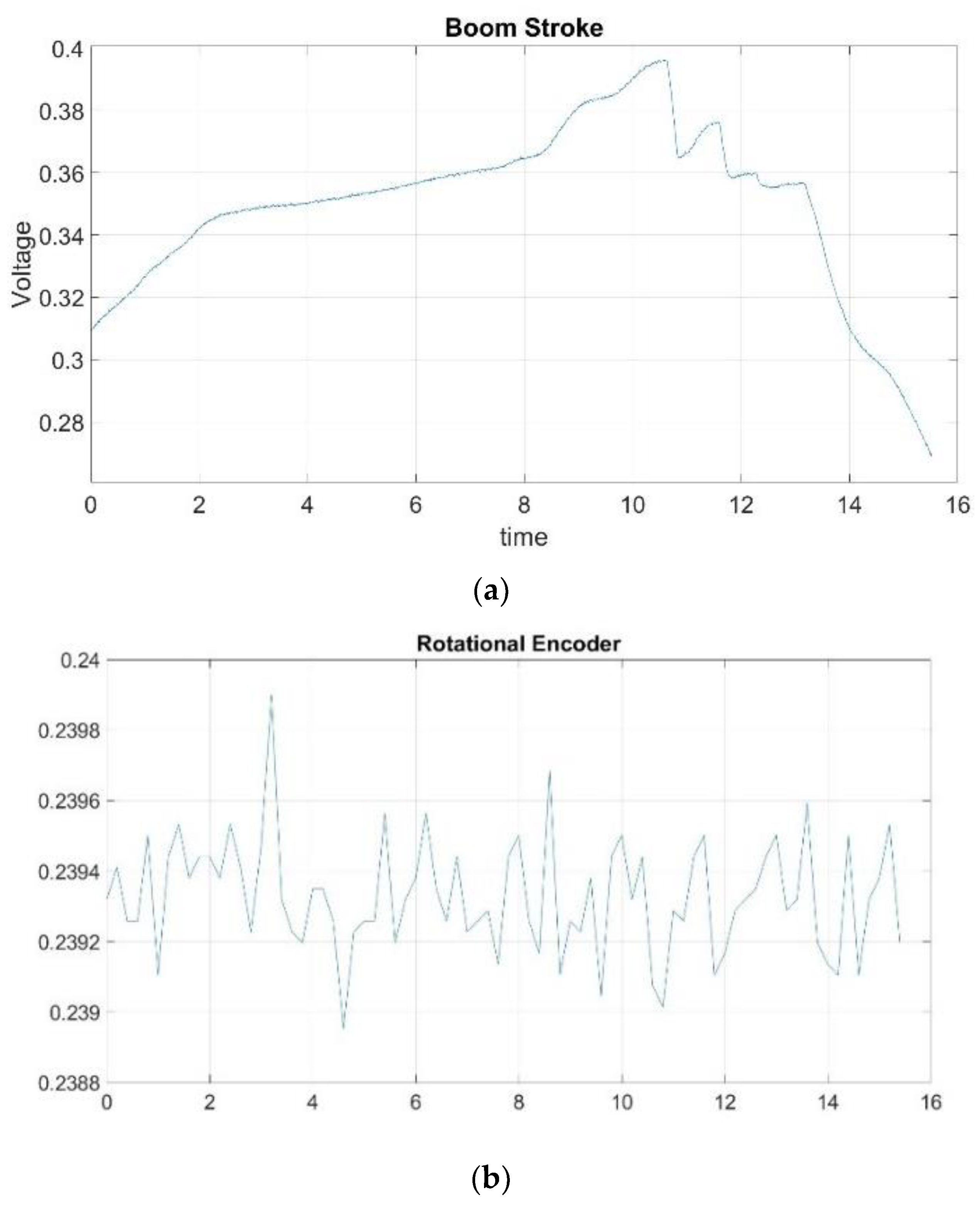
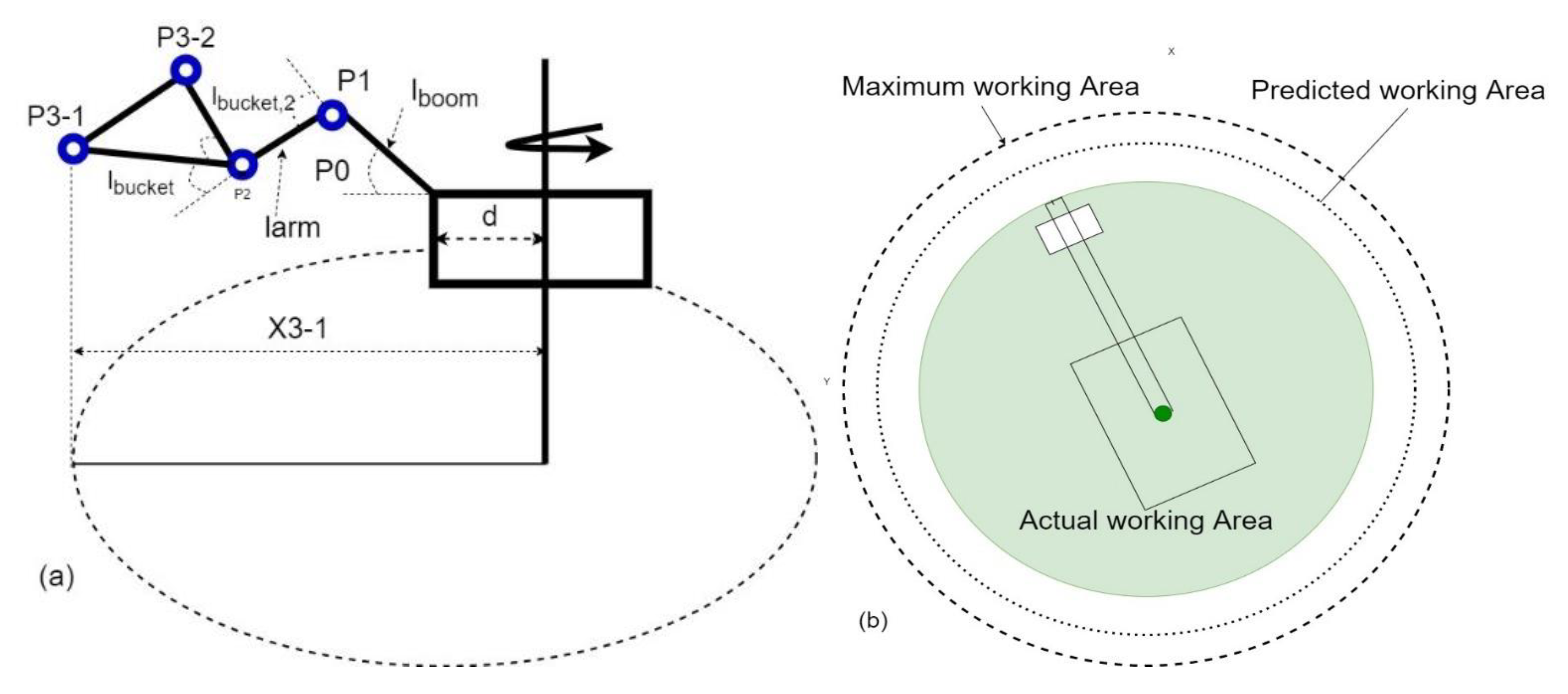
Figure 4 illustrates the positions of the boom, arm, and bucket links. Using the measurements with the stroke sensors and rotational encoder, the position of each link and the rotation of the main body were identified. Stroke sensors and the encoder were mounted on the links of the excavator and its bottom as mentioned in Section 5. Figure 5 presents the measurement data from each sensor. Using the information of the measured stroke and Equations (21)–(23), the angle of each link can be computed. Then, the application of a kinematic analysis with the angles of links enables the calculation of the predicted and actual working areas (see Figure 6).

$${\theta }_b=\pi -{\beta }_b-{\alpha }_b-{\varnothing }_b.$$

(21)

$${\theta }_a=2\pi -{\beta }_a-{\alpha }_a-{\varnothing }_a.$$

(22)

$${\theta }_{bkt}=3\pi -\mu -{\alpha }_k.$$

(23)

where $\mu =\alpha +\beta$.

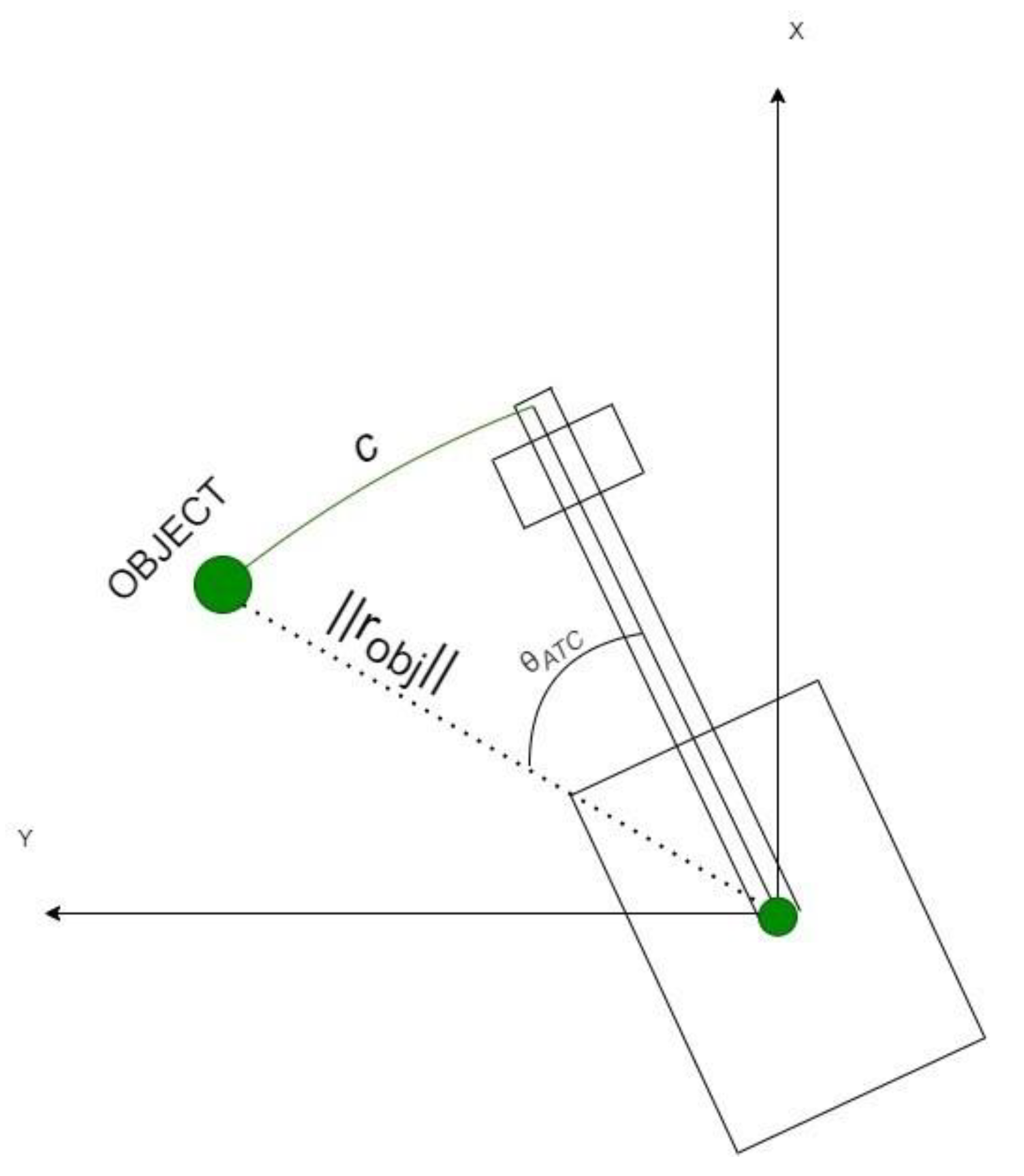
In Figure 6, $P_1$ denotes the arm joint, $P_2$ represents the bucket joint, $P_{3-2}$ is the midpoint of the bucket, and $P_{3-1}$ shows the bucket tip, $d$ shows the distance between the body center (origin of the defined coordinate system) and the boom link. The maximum working area can be achieved by the full extension of the links that can be denoted by $x_{3-1}$ (in this case, bucket tip position from the origin).

$$∆{\theta }_i=\left({\dot{\theta }}_{workingpart}+3\sigma \right)i∆t.$$

(24)

$$\left[\begin{array}{c}∆x_1\\ ∆x_2\\ ∆x_{3-1}\\ ∆x_{3-2}\end{array}\right]=\left[\begin{array}{c}{A}_{11}{A}_{12}{A}_{13}{A}_{14}\\ A_{21}{A}_{22}{A}_{23}{A}_{24}\\ A_{31}{A}_{32}{A}_{33}{A}_{34}\\ A_{41}{A}_{42}{A}_{43}{A}_{44}\end{array}\right]\left[\begin{array}{c}∆\theta boom\\ ∆\theta arm\\ ∆\theta bucket\end{array}\right].$$

(25)

where,

$$\begin{array}{l}{A}_{11}=-l_{boom}sin\left({\theta }_{boom}\right).\\ A_{21}=-l_{boom}sin\left({\theta }_{boom}\right)-l_{arm}sin\left({\theta }_{boom}+{\theta }_{arm}\right).\\ A_{22}=-l_{arm}sin\left({\theta }_{boom}+{\theta }_{arm}\right).\\ A_{21}=-l_{boom}sin\left({\theta }_{boom}\right)-l_{arm}sin\left({\theta }_{boom}+{\theta }_{arm}\right).\\ A_{31}=-l_{boom}sin\left({\theta }_{boom}\right)-l_{arm}sin\left({\theta }_{boom}+{\theta }_{arm}\right)-l_{bucket}sin\left({\theta }_{boom}+{\theta }_{arm}+{\theta }_{bucket}\right).\\ A_{32}=-l_{arm}sin\left({\theta }_{boom}+{\theta }_{arm}\right)-l_{bucket}sin\left({\theta }_{boom}+{\theta }_{arm}+{\theta }_{bucket}\right).\\ A_{33}=-l_{bucket}sin\left({\theta }_{boom}+{\theta }_{arm}+{\theta }_{bucket}\right).\\ A_{41}=-l_{boom}sin\left({\theta }_{boom}\right)-l_{arm}sin\left({\theta }_{boom}+{\theta }_{arm}\right)-l_{bucket,2}sin\left({\theta }_{boom}+{\theta }_{arm}+{\theta }_{bucket}+{\theta }_{bucket,in}\right).\\ A_{42}=-l_{arm}sin\left({\theta }_{boom}+{\theta }_{arm}\right)-l_{bucket,2}sin\left({\theta }_{boom}+{\theta }_{arm}+{\theta }_{bucket}+{\theta }_{bucket,in}\right).\\ A_{43}=-l_{bucket,2}sin\left({\theta }_{boom}+{\theta }_{arm}+{\theta }_{bucket}+{\theta }_{bucket,in}\right).\\ A_{12}=A_{13}=A_{23}=0.\end{array}$$

$$\left[\begin{array}{c}{x}_1\\ x_2\\ x_{3-1}\\ x_{3-2}\end{array}\right]=\left[\begin{array}{c}{l}_{boom}cos\left({\theta }_{boom}\right)+d\\ l_{boom}cos\left({\theta }_{boom}\right)+l_{arm}cos\left({\theta }_{boom}+{\theta }_{arm}\right)+d\\ l_{boom}cos\left({\theta }_{boom}\right)+l_{arm}cos\left({\theta }_{boom}+{\theta }_{arm}\right)+l_{bucket}cos\left({\theta }_{boom}+{\theta }_{arm}+{\theta }_{bucket}\right)+d\\ l_{boom}cos\left({\theta }_{boom}\right)+l_{arm}cos\left({\theta }_{boom}+{\theta }_{arm}\right)+l_{bucket,2}cos\left({\theta }_{boom}+{\theta }_{arm}+{\theta }_{bucket}+{\theta }_{bucket,in}\right)+d\end{array}\right]$$

(26)

$$x_{pre,p,i}=x_p+{\displaystyle \sum }_{j=1}^i∆x_{p,j}.$$

(27)

where $x_{pre,p,i}$ is the maximum value among the predicted longitudinal displacements, $x_p$ is the current longitudinal displacement, $p$ = 1, 2, 3-1, and 3-2 are the current main points of the excavator, and $i$ denotes the prediction step (1,2, …, N); $∆x_{p,j}={\mathrm{A}}_{Jacobian}∆{\theta }_i.$ The predicted angle of each part was calculated using Equation (24), which follows the Gaussian distribution, having a zero mean and a standard deviation of the noise in angular velocity. The maximum possible value of noise is $3\sigma$. $∆t$ is the discrete-time increment. i is the prediction step.

By using Equations (24) and (25), the x (horizontal position) of the point p (P₁~P_3-2) is calculated as shown in Equation (26). The predicted horizontal displacements, $x_{pre,p,i}$ can be generated using Equation (27). The maximum radius for the predicted working area is chosen from the maximum value among the predicted displacements.

Figure 6 illustrates the horizontal position of p (left subfigure) and the predicted and maximum working areas (right subfigure). One notes that the maximum working area is defined as the maximum working limit, and therefore it does not change since it can be measured by extending the three links fully. The actual working area is determined by calculating the maximum values among all x components.

4. Safety Indices and Predictive Safety Evaluation

As the required safety indices for the predictive safety evaluation, time to collision ($TTC)$ is defined as the time required for an object to collide with the excavator. The warning index, $x,$ is the normalized parameter to evaluate excavator safety in terms of distance information. To calculate the safety indices, the angle to collision, clearance, and distance between an object and the excavator should be calculated first. The safety indices are calculated based on the excavator’s current states and the object’s predicted states.

4.1. Time to Collision (TTC)

TTC is computed using the current swing acceleration and maximum swing velocity. The following equations were used to calculate TTC.

$$\left|\left|r_{obs}\right|\right|=\sqrt{x_{obj}{}^2+y_{obj}{}^2}.$$

(28)

$${\theta }_{ATC}=ta{n}^{-1}\left(\frac{y_{obj}}{x_{obj}}\right)-{\phi }_{sw}.$$

(29)

$$c=\left|\left|r_{obs}\right|\right|{\theta }_{ATC}-B_c.$$

(30)

$$\mathrm{If}{\theta }_{ATC}<0,TT{C}^{2nd}\le t_m,$$

$$TTC=\frac{{\theta }_{ATC}}{\dot{{\theta }_{sw,k}}-\dot{{\theta }_{obj,k}}}.$$

(31)

$$\mathrm{If}{\theta }_{ATC}\ge 0,t_m\le TT{C}^{2nd},$$

$$TTC=\frac{{\theta }_{ATC}+\pi }{\dot{{\theta }_{sw,k}}-\dot{{\theta }_{obj,k}}}.$$

(32)

where $r_{obj}$ in Figure 7 denotes the object’s distance to the coordinate origin, the object’s estimated coordinates are denoted by $x_{ob}\mathrm{and}{y}_{obj}$, ${\phi }_{sw}$ is the swing angle of the excavator,${\theta }_{ATC}$ shows the angle to a collision, $B_c$ is the bucket clearance, $t_m$ denotes the predicted time to reach maximum velocity, $\dot{{\theta }_{sw,k}}$ is the swing velocity, $\dot{{\theta }_{obj,k}}$ presents the angular velocity of a detected object, $TT{C}^{2nd}$ is the second-order $TTC$ that represents TTC while considering the current swing acceleration.

4.2. Warning Index (x)

The warning index, x to evaluate the excavator’s working safety is defined in terms of distance [18] and computed as:

$$c_{br}=\frac{\left|\left|r_{obj}\right|\right|\dot{{\theta }_{sw}{}^2}}{2{\alpha }_{decel,max}}.$$

(33)

$$c_{sm}=\left|\left|r_{obj}\right|\right|si{n}^{-1}\left(\frac{r_{obj,current}+u_{sensor}+u_{control}+d_{min}}{\left|\left|r_{obj}\right|\right|}\right).$$

(34)

$$x=\frac{c-c_{sm}}{c_{br}}$$

(35)

where $c_{br}$ is the braking distance, ${\alpha }_{decel,max}$ represents the maximum rotational deceleration of the main body,$c_{sm}$ is the safety clearance,$r_{obj,current}$ is the current object radius, $u_{sensor}$ is the sensor signal noise, $u_{control}$ is the control uncertainty, $d_{min}$ is the minimum clearance. $x$ is the warning index, c is the distance (clearance) between an object and the excavator. A smaller value of x indicates a higher collision risk and the excavator is required to stop its motion when x becomes one in the defined risk metric (i.e., safety level) as shown in Figure 8.

4.3. Safety Levels

For this study, three safety levels, i.e., safe, warning, and emergency braking were considered, as shown in Figure 8. The safety level is a two-dimensional parameter that is based on the calculated values of $TTC$ and $x$. Primarily, the safety level is the time and distance to a collision.

The excavator can continue working without any risk under the safe region. Alarm signals are generated in the warning region for an operator to recognize a hazardous situation. Finally, immediate braking needs to be applied at maximum deceleration to avoid any collision in the emergency region.

5. Experimental Results

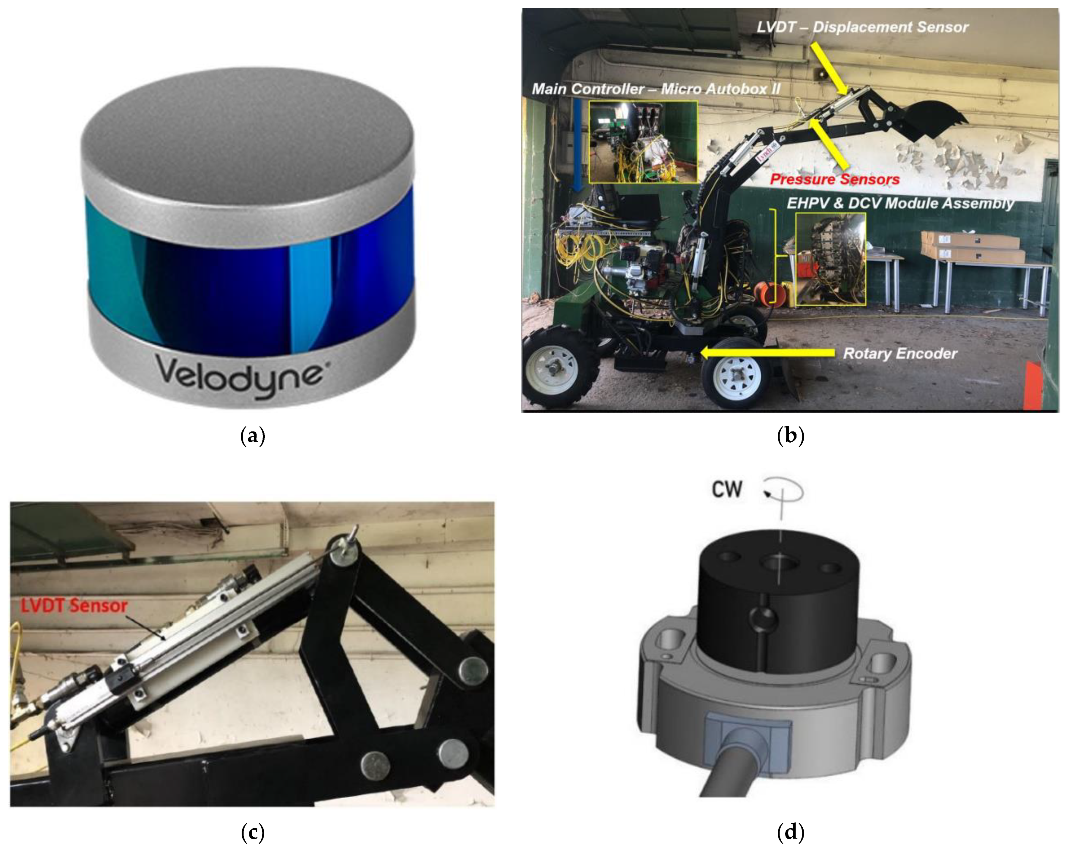
A LiDAR sensor (Velodyne VLP-16) in Figure 9a was used to detect objects around the excavator during experimental tests. Data obtained from the LiDAR was post-processed with MATLAB whose libraries allow us real-time processing.

The algorithms were tested on the autonomous mini excavator at AVEC lab (Ontario Tech University) shown in Figure 9b that was modified from an existing manual type excavator (RMD 500, Yantai Rima Machinery, Yantai, SD, China, 2020) by implementing a HW controller (dSPACE), valve blocks, and several types of sensors.

The developed test platform excavator was comprised of three subsystems, i.e., hydraulic, electronic, and mechanical systems. The hydraulic subsystem consisted of electro-hydraulic proportional valves (EHPVs), directional control valves (DCVs), a hydraulic reservoir, hydraulic actuators, and a hydraulic pump. The electronic subsystem was composed of a power supply, relay box, pressure sensors, LVDT stroke sensors (Figure 9c), and a rotary encoder (Figure 9d). The mechanical subsystem was made up of three links (boom, arm, and bucket) and the main body.

5.1. Experimental Test Scenario

Experiments were carried out in the presence of multiple static objects, as well as moving ones that were walking around the excavator to represent a collision scenario.

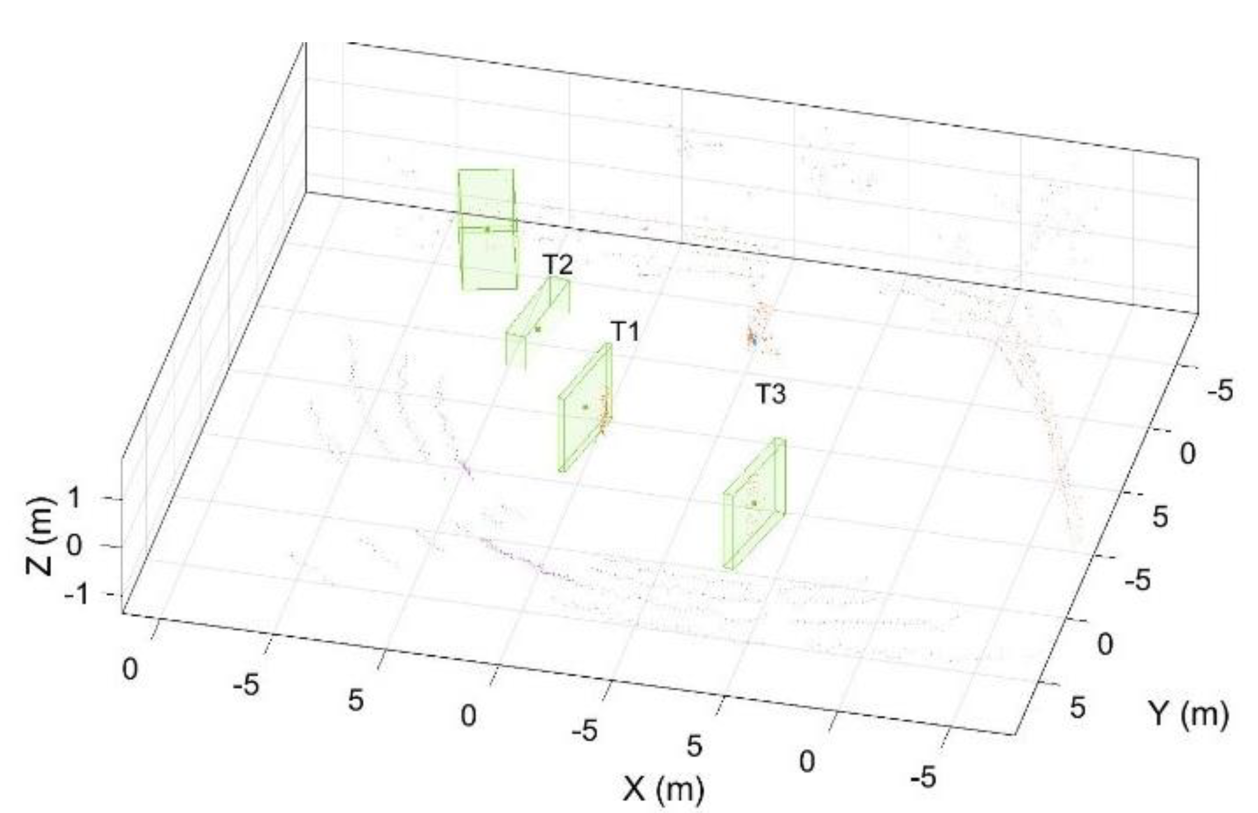
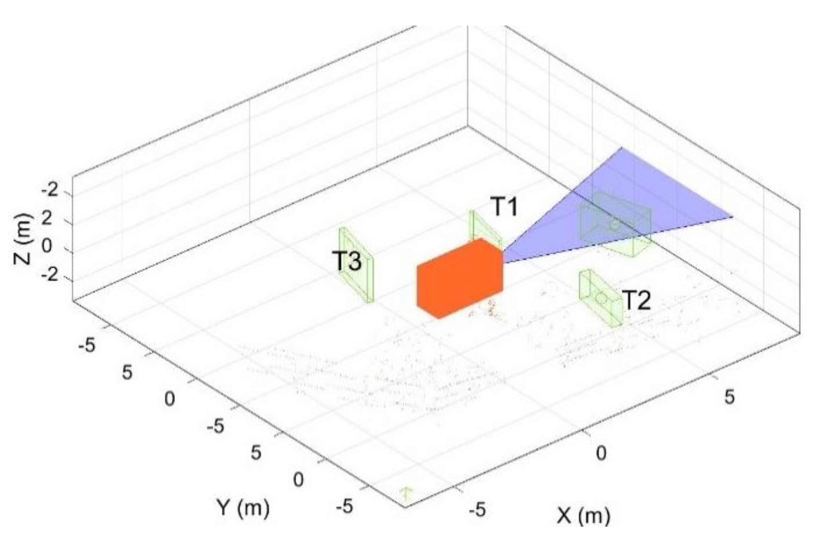
In Figure 10, one monitored static object T2, and two moving objects, T1 and T3, are indicated. The objects present in the ROI carry their unique labels. If an object leaves the ROI, its corresponding label is deleted, and a new label will be assigned upon returning to the ROI. Therefore, some labels in Figure 10 are missing because the objects that had left the ROI did not present in the ROI anymore. As the object enters the ROI and continues to move closer to the excavator, object detection, tracking, and safety evaluation are performed.

Note that some points in Figure 10 are not clustered at the current time frame due to the issue of processing time. Therefore, these points may be in a cluster formed after a few frames.

5.2. Results

Figure 10 shows the raw point cloud data for detected objects. Note that every object has its unique label that helps track management to associate data to each detected object ($T1,T2,$ and $T3$). This could also help in counting the number of objects around the excavator.

Figure 11 presents the operator’s view to see the excavator and moving objects ($T1,T2,$ and $T3$) around it. The box (orange color) and fan shape (purple color) in the figure represent the excavator and the operator’s visible sight, respectively. The bounding boxes denote the objects around the excavator. The track IDs in Figure 10 and Figure 11 are identical to maintain unique labels for the objects.

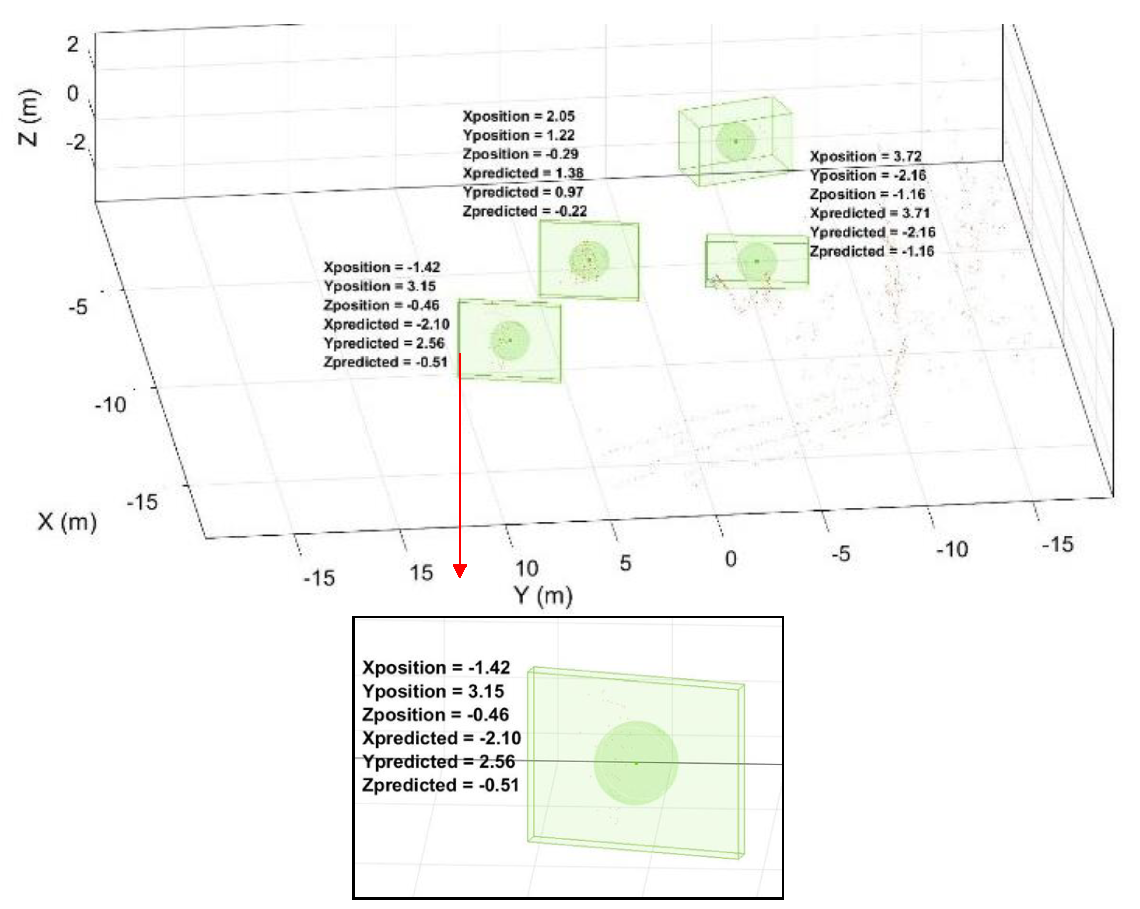
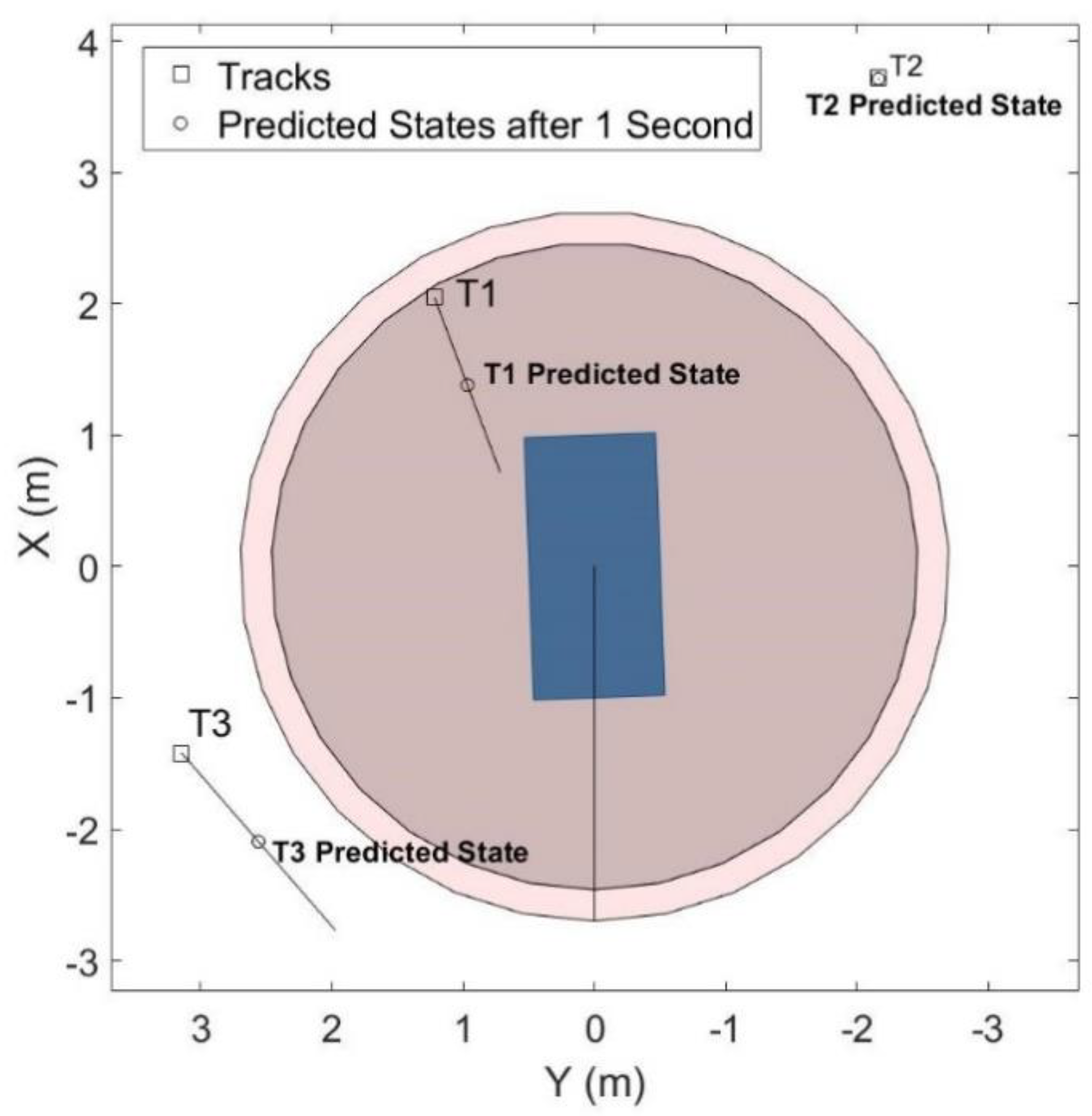
The detailed tracking results are presented in Figure 12 that includes the information of the $x,y$, and $z$ coordinates of each object. These coordinates indicate the current and predicted (1 s ahead) positions of the detected objects. The tracking details were utilized for object tracking and safety evaluation. In Figure 13, the maximum and the actual working areas of the excavator are shown. It also shows the rotation angle of the excavator, the heading angle of tracked moving objects, and their current and predicted states.

The current area of work represented by the inner circle was obtained by conducting the kinematic analysis, while the maximum working area was achieved through a full extension of three links. The safety indices were calculated based on the actual working area. Note that $T2$ is the static object, and thus its predicted and current positions did not change.

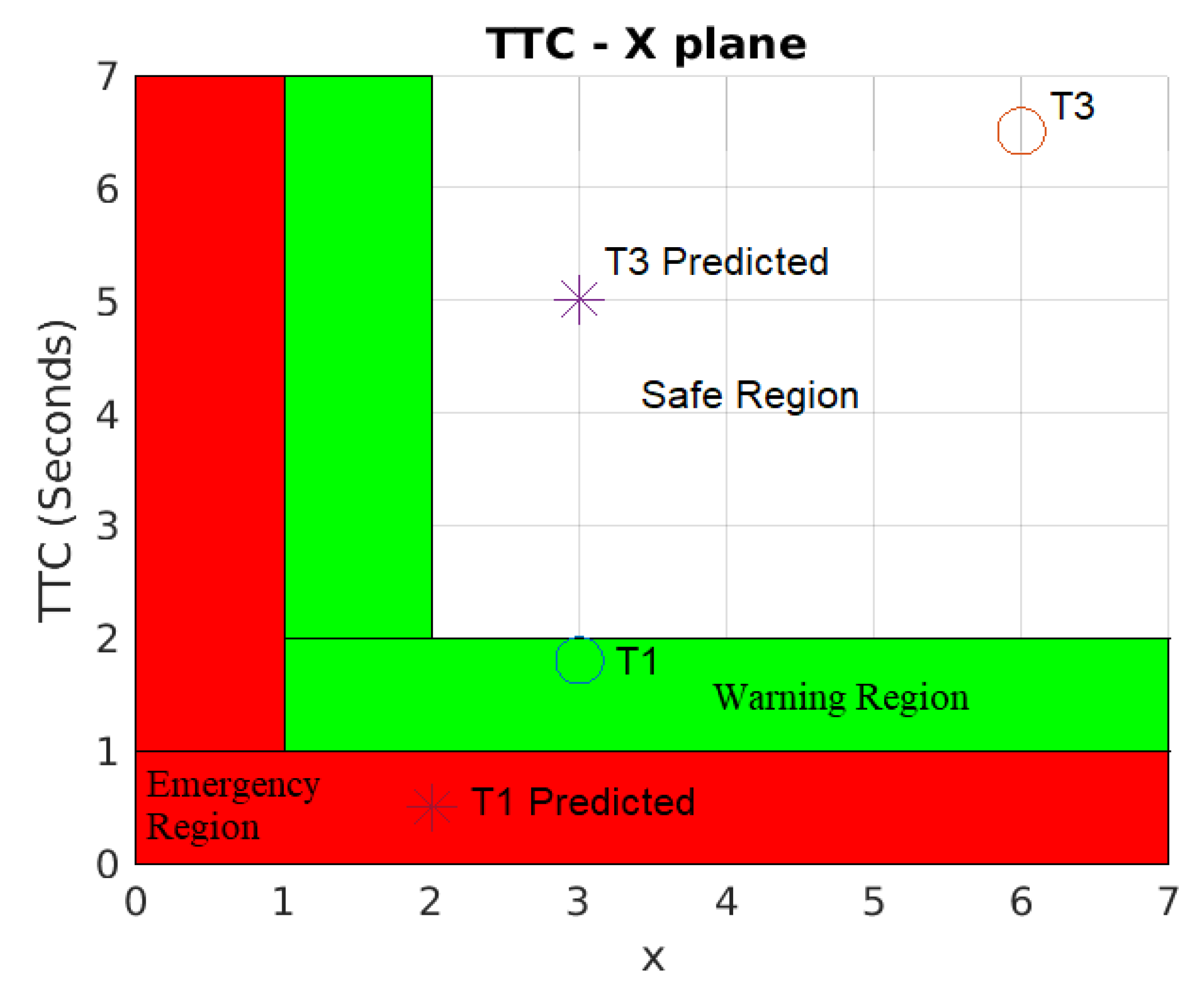
Figure 14 shows the results of the safety evaluation results computed with the safety indices presented in Figure 8. The current states of T1 and T3 with a circle mark are in the warning and safe regions, respectively. However, the predicted state (1 s ahead) of T1 with the × mark indicates that it is entering the emergency region, and thus the chance of collision has highly increased. Therefore, immediate braking should be taken in 1 s to prevent a collision accident for T1 since TTC is less than 1 s. All the detected static objects were far from the maximum working area in the test scenario (i.e., no potential hazard exists in this case), and thus only moving objects are included for the safety evaluation, as seen in Figure 14. Monitoring in Figure 13 and safety evaluation in Figure 14 can work synchronously (see the attached video clip).

Finally, the performance of the developed safety algorithms was evaluated in terms of prediction accuracy using the same experimental data from the test scenario in Figure 13 and Figure 14. For this evaluation, we compared the predicted positions of the moving objects T1 and T3 at each time frame with the actual positions 1 s after prediction. Since the minimum Euclidean distance for clustering (i.e., the minimum size of a bounding box to detect moving objects) was set as 0.4 m (average of a worker’s chest size), this value was determined as a threshold to judge the success or failure of the prediction. Specifically, the prediction is recognized as ‘success’ if the error between the predicted and actual positions at each time frame (0.1 s) per object is smaller than the threshold value.

Table 1. Evaluation of prediction accuracy of the developed safety algorithms.

	T1	T3
No. of time frames with successful predictions	220	250
No. of total time frames	258	298
Successful operation (prediction) rate, %	85.27	83.89
Average error, m	0.29	0.28

includes evaluation results to show a successful operation (prediction) rate for each object achieved by the developed algorithms. During the considered test scenario, the successful operation rate for T1 was 85.27% to indicate that the error is less than the threshold in 220 time frames out of the total, 258. The average error across all the time frames (258) was 0.29 m for T1. However, the successful operation rate for T3 was slightly lower (83.59%) than the case of T1, and its prediction accuracy was more or less increased with the decreased average error of 0.28 m. Therefore, it is noted that the proposed algorithms provide satisfactory performance on position prediction in most of the given time frames.

6. Conclusions

This study proposed sensing algorithms for object tracking and predictive safety evaluation for an autonomous excavator that effectively enables us to avoid potential collision risks between the excavator and the workers around it. Firstly, the proposed method extracted non-ground points from raw point cloud data with 3D LiDAR. The non-ground points were then clustered, and each cluster was fit into a bounding box that was considered as a detected object. The positions and velocities of the detected objects were then estimated and predicted using the integrated tracking filter where the JPDA for multi-target tracking was coupled with UKF and IMM to improve the performance of the tracking management by dealing with the non-linear state estimation and different motion behaviors (i.e., constant velocity and constant turn models), respectively.

The developed algorithm can also monitor the current working areas of the excavator and predict them to conduct safety evaluations. The defined safety indices, $TTC$ and $x$ were computed through the prediction of the motion of the detected objects and calculation of the working areas of the excavator based on kinematic analysis. The severity of potential collision risks was defined using the safety indices.

Validations of the developed algorithms were performed with a modified mini excavator having a VLP-16 3D LiDAR, LVDT stroke sensors, and a rotational encoder. Test results indicate that the proposed predictive safety algorithms can successfully conduct tracking of objects, predict their motion, and provide safety evaluations to prevent a collision accident.

A novel feature of the developed safety strategy is the ability to predict the future states of both multiple objects and an excavator within a prediction horizon (i.e., 1 s in advance) during operations. Since previous studies of construction equipment have focused on monitoring its present state, the predictive attribute of this study, conceptualized through a risk metric with time and distance to potential collisions, is the most significant advance, and it will be used to control autonomous excavation equipment that requires more elaborate and precise safety strategies. As part of the evaluation of the developed safety algorithms, this work provides a unique methodology for defining a threshold for judging success or failure predictions and analyzing the success rates of operations with respect to time frame. Therefore, the study proposes an advanced safety management framework that can be applied to many industrial applications, such as construction equipment in transition to full automation and/or autonomy, in which predictive safety is a prerequisite component.

As the constant velocity and constant turn models were assumed for the prediction of the moving objects in the tracking filter, the application of the variable velocity and random motion models will assist in improving the performance of the safety algorithms in predicting the nonlinear motions of the objects in future work. System dynamics [25,26] can also be considered for an extension of the current work to enhance the predictive capability of the developed algorithms by investigating the interrelations among the factors causing safety incidents, such as worker-machine interaction.

Excavator safety can be improved by pairing the proposed safety algorithms with the development of sophisticated sensing algorithms or platforms that can avoid the restricted FOV and occlusions caused by obstacles in excavation spaces. Finally, a further advantage of state prediction is that the actuators of an autonomous excavator can be controlled in an adaptive manner depending on the degree of potential collision risk, thereby providing maximum productivity and safety over simply stopping the excavator.