
Theoretical Modelling of Ion Exchange Processes in Glass: Advances and Challenges


Quantum Materials and Photonics Research Group, Optics Area, Department of Applied Physics, Faculty of Physics/Faculty of Optics and Optometry, Campus Vida s/n, Universidade de Santiago de Compostela, E-15782 Santiago de Compostela, Galicia, Spain
*
Author to whom correspondence should be addressed.
Appl. Sci. 2021, 11(11), 5070; https://doi.org/10.3390/app11115070
Submission received: 20 April 2021
/
Revised: 19 May 2021
/
Accepted: 24 May 2021
/
Published: 30 May 2021
(This article belongs to the Special Issue Ion-exchange in Glasses and Crystals: from Theory to Applications )
Abstract
:In the last few years, some advances have been made in the theoretical modelling of ion exchange processes in glass. On the one hand, the equations that describe the evolution of the cation concentration were rewritten in a more rigorous manner. This was made into two theoretical frameworks. In the first one, the self-diffusion coefficients were assumed to be constant, whereas, in the second one, a more realistic cation behaviour was considered by taking into account the so-called mixed ion effect. Along with these equations, the boundary conditions for the usual ion exchange processes from molten salts, silver and copper films and metallic cathodes were accordingly established. On the other hand, the modelling of some ion exchange processes that have attracted a great deal of attention in recent years, including glass poling, electro-diffusion of multivalent metals and the formation/dissolution of silver nanoparticles, has been addressed. In such processes, the usual approximations that are made in ion exchange modelling are not always valid. An overview of the progress made and the remaining challenges in the modelling of these unique processes is provided at the end of this review.
1. Introduction
Ion exchange in glass has been used for centuries for the purposes of decoration and colouring. Glass lustre on ceramics with metallic nanoparticles from ion exchange has been known from the early Islamic culture during the 10th Century [1]. However, the scientific and industrial application of this technique dates back 60 years ago when potassium ion exchange (IE) was first applied in the chemical surface tempering of glasses [2,3]. Next, with the introduction of the concept of integrated optics in 1969 [4], ion exchange in glass was proposed as a waveguide fabrication process. Just a few years after this proposal, Izawa and Nakagome published the first work on ion exchange waveguides [5]. This kind of waveguide presents several advantages: fibre compatibility, low propagation losses and low cost. Moreover, ion exchange can be combined with other techniques, such as sol–gel, for the fabrication of passive and active (rare-earth-doped) integrated optical devices [6]. Currently, the main applications of ion exchange are in glass strengthening [7,8,9,10,11] and in the fabrication of photonic components for both guided-wave [12,13,14,15,16,17,18] and bulk optics [19,20,21].
In an IE process, cations (mostly ) close to the glass surface are replaced with other monovalent cations such as , , , , or [22]. Molten salts of such cations are common sources of dopants, although a metallic film deposited on the glass surface can be also a source of cations. The exchange takes place by a purely thermal diffusion process or it can be assisted by an electric field. The new cations can change the electrical permittivity, the stress and even the absorption of the glass, these being changes proportional to the dopant cation concentration. By selective masking of the glass surface, ion exchange can be locally prevented or allowed, giving rise to custom-made elements for specific purposes. The theoretical modelling of the IE processes ran parallel to the development of the technologies. This modelling was fundamental to the design and fabrication of most elements. For instance, in the field of integrated optics, some subjects as fibre compatibility or coupling losses depend strongly on the permittivity distribution and, hence, on the cation concentration. Therefore, the prediction of the cation concentration is of great importance to design devices based on IE technologies.
Here, we present a review of the theoretical modelling of IE processes in glass made up to now, as well as the last advances in this matter that have been reported in recent years. Ion exchange within a glass network is governed by diffusion and drift processes as a response to a concentration gradient and an electric field, respectively [23,24]. This gives rise to a concentration profile of the exchanging ions, which depends on the processing conditions of the substrate: temperature, exchange time, applied electric field, etc. The Nernst–Planck drift-diffusion equation describes this process. It establishes the proportionality among the flux density of each ion species and both the electric field and the concentration gradient. On the other hand, Poisson’s equation and continuity equations for each ion must be fulfilled. This gives rise, in general, to three second-order coupled partial differential equations whose solution provides the evolution of both the cation concentrations and the electric potential. In the derivation of these equations, the charge neutrality approximation is usually assumed, which allows for some important simplifications without a relevant loss of accuracy in the most common cases [25,26]. All of these subjects are addressed in Section 2, where we present the basic model of ion exchange. This model assumes that the self-diffusion coefficients of the exchanged cations are constant for a given temperature. However, experimental measurements [27] showed that these coefficients depend on the cation concentrations. Therefore, this basic model was generalized to non-ideal cation behaviour and concentration-dependent self-diffusion coefficients by considering the so-called mixed ion effect [28,29]. Later, both models were rigorously generalised, and in the derivation of the equations, Faraday’s law was considered instead of Ohm’s law [30]. This leads to a non-standard Laplace equation for an effective electric potential. Accordingly, the boundary conditions for the most common IE processes were established. These conditions, together with the aforementioned partial differential equations, complete the theoretical modelling of the IE problem. On the other hand, some IE processes have attracted a great deal of attention in the last few years due to their remarkable applications. Among these, we must highlight: glass poling, electro-diffusion of multivalent metals and the formation/dissolution of silver nanoparticles. Their modelling has only been partially done so far [31,32,33], because the usual theoretical assumptions (mainly charge neutrality approximation and ideal cation behaviour) are not always valid in such processes. In Section 4, we give an overview of the progress made and the challenges still to be faced on this matter.
2. Basic Model
The simplest problem of ion exchange arise when two species of monovalent cations (A and B) exchange with each other in the same glass region at a given temperature T. Let us consider an infinite one-dimensional medium (x being the spatial coordinate) with a homogeneous concentration of fixed anions (typically -Si- radicals) and non-homogeneous and variable cation concentrations and , t being the time. Moreover, we considered that each cation is initially near its anion, that is they are paired, so . Consequently, space charge density is initially cancelled:
that is local charge neutrality is met. Our goal was to obtain the evolution of cation concentrations given these initial conditions.
2.1. Nernst–Planck and Poisson Equations
The initial non-homogeneity of cation concentrations, and , and their random motion make them diffuse along the glass until their concentrations are homogeneous. This diffusion process is described by Fick’s law:
where is the flux density and the diffusion coefficient of each cation. However, the two interdiffusing cations have usually different diffusion coefficients and, therefore, different mobilities, which produce charge imbalances. These imbalances generate a strong internal electric field (), which tends to balance the charges and restore charge neutrality (Equation (1)). Therefore, Fick’s equation is no longer valid, and a drift term must be added on its right-hand side to take into account the effect of this electric field on the cation motion. This leads to the Nernst–Planck equation [34]:
where e is the proton charge, T the absolute temperature and k Boltzmann’s constant. Note that some authors included, in the drift term of this equation, the Haven ratio. However, as we will see below, this parameter should not be incorporated into the model as a general rule. The occurrence of the above-mentioned electric field can be seen from a quantitative point of view by calculating the total flux density:
which depends on the electric field through mobility u:
However, cancels in the current problem, that is,
because there is no external field applied that generates a net current. This means that the imbalance of the diffusion of the two cations () is compensated by the internal field through the drift term . Note that Equation (4) is a generalization of Ohm’s law. On the other hand, as long as there is no creation or destruction of cations from/to a metallic state, the continuity equation must be fulfilled:
Now, by combining this equation and Equation (3) for, for instance, i=A and substituting, in the resulting equation, the electric field from Equations (4) and (6), we obtained the differential equation that gives the concentration evolution [23] of cation A:
where the charge neutrality (Equation (1)) was applied and a normalized concentration () was used, and we defined the following interdiffusion coefficient:
where . The dependence of u and on predicted by this basic model, for / IE, can be seen in Figure 1a.
A more complex problem is the IE assisted by an external electric field. In such a case, Equation (6) is not met. Therefore, additional equations are necessary to calculate the total flux density () or, alternatively, , which now includes the external field. As for , it must fulfil Poisson’s equation and Faraday’s law of induction:
where is the glass electrical permittivity and is the magnetic field, which will be assumed as time independent since the total current changes very slowly. On the other hand, we also assumed the charge neutrality approximation (Equation (1)). This cannot be done in general, due to the existence of the aforementioned external field; however, in most cases, this is a very good approximation (see the next subsection). Doing this, the addition of continuity Equation (7) leads to:
Now, by finding the electric field in Equation (4):
taking into account Equation (12) and doing the same steps as before, the following electro-diffusion equation is obtained:
which is an extension of Equation (8). On the other hand, Equation (13) can be inserted into (11), leading to:
where we used Equation (9). This equation, Equation (12), and the boundary conditions, which will be presented later, determinate the flux density . From this flux density, Equation (14) will provide the evolution of the concentration of cations. Finally, once and are known, the charge neutrality approximation can be checked. This will be analysed in the following subsection.
Alternatively, the last four equations can be expressed in terms of a scalar function. Indeed, an irrotational vector field is the gradient of a potential function , so:
where the factor was included in order for to have the same units as the electric potential. From this equation and Equation (12), we obtained a non-standard Laplace equation:
which is more convenient for resolution purposes than vector Equations (12) and (15). Note that this effective potential is not the electric potential V, whose minus gradient is the electric field given by Equation (13). However, a relationship between them can be obtained [30] by inserting Equation (16) into Equation (13), that is:
Under typical IE conditions, the difference between V and is no greater than a few tenths of a volt, which is negligible compared to the usual voltages (20–100 V) used in field-assisted IE. Despite this, this difference must not be ignored in the modelling, as significant errors in the calculation of the electric field could be made. Indeed, although both potentials are similar, their gradient is not always.
On the other hand, it is worth mentioning that Equations (12) and (15) are trivially solved in the one-dimensional case, that is is constant. This constant will be established from the experimental setup. If a constant current source is used, this value is set directly. Otherwise, when the external field is generated by a constant voltage source, the value of can be calculated from the voltage applied to the sample and Equations (14) and (16)–(18).
2.2. Charge Neutrality Approximation in Field-Assisted Ion Exchange
In the previous subsection, the charge neutrality was assumed in the field-assisted IE problem, as well as in the thermal-only case. However, this charge neutrality is not always fulfilled, especially when strong external electric fields are used and/or very high concentration gradients exist. In fact, some authors have modelled the silver concentration in channel waveguides by considering explicitly the space charge distribution [35], albeit at the cost of including other assumptions.
An estimation of the validity of the charge neutrality approximation can be made from Equation (13), which can be expressed as:
where we used the charge neutrality approximation and the definition of . Now, we took divergences in this equation in order to compare it with Equation (10) and estimate the error made by this approximation. This is an iterative procedure. First, we used this approximated expression for the electric field. Next, we substituted it into Poisson’s Equation (10) to obtain a more accurate value for , which was introduced in the previous equation, and so on. However, a unique iteration will be enough to obtain an order of magnitude of the charge density [36]. Therefore, if we use Equation (12) and assume that does not depend on and , we obtained:
Now, from this equation, we can obtain some conditions for the validity of the charge neutrality approximation by comparing each term on the right-hand side of this equation with the second term on the left-hand side. Therefore, for the second term on the right-hand side, this comparison provides:
for a BK7 glass with a density of 2.4 g/ and 8.4% by weight of O, which gives ; likewise, typical values for the temperature, T = C, and for the relative permittivity, = 10, were considered. As for the ion exchange, we chose for this assessment a / IE in a soda-lime glass with a diffusion coefficient ratio [37], which leads to = 0.975. Therefore, must fulfil the following condition:
In the worst case, = 1. This condition means a change, in the normalized concentration, from one to zero-point-nine at a distance much greater than 0.36 nm, which in practice is met in almost any IE process. Indeed, most IE processes use glasses with a higher O content or their values are less than the one of / IE. Therefore, this condition is even less restrictive in those cases.
On the other hand, the third term on the right-hand side of Equation (20) is small under the same conditions as the second one. Finally, the first one is small if the second one is and, furthermore, if:
where we took into account [37] that /s, for T = C. That is, in the worst case ( = 1), the current density must fulfil:
This condition is ensured in practice because the highest current densities that have been used in field-assisted IE processes until now are much lower than this value. In fact, Joule heating should be taken into account for currents higher than a few mA/, due to the strong dependence of diffusion coefficients on the temperature [38,39]. Therefore, the charge neutrality approximation is valid in most IE process, even for / and / ion exchanges, which give rise to very steep concentration profiles. In these kinds of profiles, although may be very high, the denominator of Equations (21) and (23) is not close to zero, even for molar fractions close to one. Indeed, we assumed that is constant, but actually, the diffusion coefficients depend on the molar fractions, so that if a cation has a low concentration, it also has a lower diffusion coefficient. In other words, if , then < 0, and is never close to zero. The basic model that we present in this section cannot explain these dependencies on the concentration of the diffusion coefficients, and therefore, this cannot be used to describe the whole range of molar fractions.
2.3. Boundary Conditions
When an external medium is in contact with the glass surface, each type of cation present in the glass and/or in the medium can either cross or not cross the glass/medium interface. This depends on the nature of such a medium. If a cation crosses the interface, a thermodynamic equilibrium is assumed between the crossing cations at both sides. Otherwise, the normal component of its flux density cancels. Therefore, the different boundary conditions for the Equations (14), (16) and (17) are obtained for a mask/air, a silver or copper film and a molten salt mixture, when none, one or both cations, respectively, cross the interface. Moreover, when the external medium is a conductor (metallic film or fused salt), its electric potential can also be chosen and directly affects the boundary condition of the potential through Equation (18).
In Table 1 and Table 2, we summarize the boundary conditions for IE processes from molten salt mixtures and films, as well as under a mask or in air. The equations that govern these processes are also shown. Note that boundary conditions for other common IE processes as annealing or secondary ion exchanges are included in these cases. Indeed, boundary conditions for annealing processes are the same as for “mask/air”, and the ones for secondary ion exchanges are included in the “salt” case, just using a different constant “C”, which depends on the dopant concentration in the salt mixture and temperature through an equilibrium equation [40,41,42,43]. Moreover, the final concentration of the first process is the initial condition for the second one.
We show, in these tables, the two alternative forms presented in Section 2.1. In Table 1, the problem is formalized in terms of the normalized concentration of dopant cations and the total flux density . This is a more straightforward form, which makes it easier to understand the physical problem of ion exchange. However, for resolution purposes, the form given in Table 2 is simpler because it is written in terms of and a scalar function , which can be seen as an effective electric potential [30].
The basic model of this section implicitly assumes an ideal cation behaviour in the glass. Therefore, for the sake of consistency, the same assumption was made in the electrochemical potentials to obtain the theoretical equations for the boundary conditions of Table 1 and Table 2. However, the corresponding condition for in a glass–salt interface, as a function of the salt composition, must contain non-ideal terms on the glass side, as we will show in the next section. Owing to the molten salt being homogeneous, is constant along the surface. Hence, a mixed theory can be a pragmatic approach; similarly, experimental values for can be used to feed the numerical algorithms that model the ion exchange. On the other hand, the boundary conditions for are sometimes irrelevant (thermal diffusion) or they can be approximated to those of V (diffusion assisted with strong fields). As a result, they were often ignored in models and experiments in the context of waveguide fabrication.
2.4. Some Particular Solutions
Two noticeable one-dimensional solutions are obtained for both specific thermal and field-assisted IE processes. In the simplest thermal IE, a glass sheet is immersed in a molten salt, which contains foreign cations. The boundary conditions for and are constant over time and along the glass surface, then . The concentration profile of the dopants scales in depth proportionally to the square root of the diffusion time, but it retains its shape, that is , being the origin of the coordinates at the glass surface [44]. The shape of f depends on and . If either of them is small, the diffusion Equation (14) becomes linear and f tends to a complementary error function (), which has an inflection point at the glass surface and decreases monotonically to zero inside the glass. Otherwise, the diffusion is faster near the surface, where the dopant concentration is high. This causes f to present a bump near the surface, being the inflection point displaced into the glass. f is often approximated by a Gaussian function, although other functions have been proposed [45,46,47].
When a voltage is applied between both surfaces of the glass sheet, a current normal to these surfaces appears. If is kept constant, a stationary solution of Equation (14) exists when the slow cations invade a region containing a higher concentration of fast cations [24]. In that case, the mole fraction profile of the slow cations is a step-like function that moves at a constant speed while maintaining its shape. Therefore, two regions with different concentrations are formed with an abrupt transition between them. The higher the step is, the sharper the front and the greater its velocity because the mobility of slow cations increases with its concentration. The stability results from a competition between diffusion and the non-linearity of the drift term. The former widens the profile, whereas the latter sharpens it because the rear region of the profile moves faster. On the other hand, if V is kept constant, decreases slowly over time, since the resistivity of the sample increases as the doped region becomes thicker. This effect may already be appreciable for doped regions a few microns deep, because the mobility ratio can reach several orders of magnitude [38,48]. In [38], the applied voltage V had to be corrected by 0.93 V to accurately describe the experimental depths because these models did not include the potential . Note that a combination of the boundary conditions of at both glass sides, as well as the difference between and V given by Equation (18) explain such a potential. Finally, it is worth noting that a stable profile is only formed if the slow cation chases the fast one. Otherwise, the profile extends indefinitely.
3. The Mixed Ion Effect
Constant diffusion coefficients were assumed in Section 2. However, they depend on both the temperature T and the molar fraction . In monoalkaline glasses, the temperature dependence follows the Arrhenius law:
This is due to each cation needing to surmount a potential barrier of height equal to Q to move to another potential well. The diffusion coefficient is proportional to the number of cations that overcome this energy in a given instant. This number follows a Maxwell–Boltzmann statistic, which explains the above exponential law. According to the Stuart–Anderson model [49], the potential barrier has both an electrostatic component, corresponding to the energy necessary to separate the cation from its anion, and a mechanical component that describes the glass network distortion necessary for the cation to break through another potential well. Therefore, when two species of cations are present in the glass, it is natural that each one has its own diffusion coefficient. However, surprisingly, the and Q values of each species (, and , ) largely depend on the cation mole fraction, in such a way that each diffusion coefficient is reduced by up to several orders of magnitude as its respective mole fraction is approaching zero [27,50,51]. This reduction is mainly due to an increase of the activation energy of minority cations; furthermore, it is stronger than the difference between the diffusion coefficients of both species in their respective monoalkaline glasses ( and ). Consequently, and are equal for some intermediate mole fractions. We will show that this leads to a maximum value of the interdiffusion coefficient and a minimum value of the direct current (DC) conductivity for this intermediate mole fraction or its neighbourhood. Therefore, the DC conductivity shows an excess of activation energy with respect to the monoalkali glasses (this excess disappears with frequency in AC conductivity). This phenomenon, among others, is included in the so-called double-alkali effect, mixed alkali effect or, later, mixed mobile ion effect or mixed ion effect (MIE), since silver, thallium or copper cations behave similarly to alkali ones in glass [37,52,53,54].
3.1. Brief Review of Theories
The origin of the MIE has been debated for a long time, but no theory has been universally accepted yet. Some theories focus on an interaction among neighbouring cations in such a way that mixed pairs are assumed to be more energetically stable than pairs of cations of the same species [15,55,56,57,58,59]. This assumption is supported by several experimental achievements. Namely, the interdiffusion coefficient presents a thermodynamic term for alkali IE [60,61] and for / exchange [62]; we will show that this term is missing if cations behave as an ideal gas. Furthermore, the surface mole fraction of cations in ion exchanged glasses from molten salts (the salt boundary condition) must be explained on the assumption that a non-ideal cation behaviour both for double-alkali exchange [40,41] and for / exchange [42,43]. On the other hand, mixing enthalpy experiments do not have a clear interpretation. A negative mixing enthalpy (net attraction among dissimilar cations) was found [63,64,65], which correlates linearly with the excess of activation energy for DC conduction. However, the former is about 20 times weaker than the latter. Besides, mixed pairs of cations would be expected to be much more likely than pairs of the same species in the presence of interaction, but nuclear magnetic resonance experiments [66,67,68], as well as neutron and X-ray diffraction [69] show that they are rather randomly distributed. Consequently, other authors attributed the MIE to relaxation processes in the glass structure [70,71,72,73]. In particular, each cation is assumed to modify its neighbourhood after a relaxation time to achieve an energetically favourable site. Therefore, in a monoalkaline glass, all the sites are of the same type. Once a foreign cation enters this glass and modifies a site, it is difficult for it to diffuse because all accessible sites are the wrong type. Even if the cation gains access to one of them, most likely, it will return before the new site relaxes. Moreover, diffusion is assumed to occur through conduction pathways, so a foreign cation can block several indigenous ones. This explanation is compatible with the ideal behaviour of cations, that is with a random distribution.
The theory that we assumed is relevant because, depending on it, the resulting diffusion equation is slightly different, as we will show below.
3.2. The Cation Flux Density
Let us consider the electrochemical potential () of each cation species that has a chemical term depending on the thermodynamic activity () of that species and an electric term proportional to the cation charge (e) and the electric potential (V):
The flux density of each cation species is proportional to both the gradient of its electrochemical potential and its concentration. This leads to the Nernst–Planck equation:
where the ’s are the thermodynamic factors:
As mentioned above, some authors include the Haven ratio in the drift term of Equation (27). However, the Haven ratio should only be used to obtain from the experimental values of the diffusion coefficient of radioactive tracers: [74]. The difference between them arises, for example, if the diffusion mechanism is the indirect interstitial one. In this case, a cation located in one interstice replaces a nearby regular site cation, which jumps to another interstitial site. Consequently, the total mass (or charge) displacement described by is different from that of a single cation, which is measured by the tracer. Moreover, the tracer is also affected by the thermodynamic factor, then a comparison between the mobility of a species and the corresponding tracer diffusion coefficient can result in an apparent Haven ratio [61].
If the MIE is fully due to the relaxations of the glass structure, the cation behaviour being ideal, the activity will be equal to the mole fraction, so . On the contrary, if the cation interaction is the only thing responsible for the MIE, we will obtain , being the thermodynamic activity coefficient (). Let us deduce that result. We divided all cations A into two sets, the ones that are hopping from one site to another in a given instant () and the rest of them, which are fixed (). Although the former are much scarcer, both sets are in thermal equilibrium in any given small region in the glass; therefore:
Now, we made two assumptions. First, we supposed that mobile cations behave ideally with respect to each other due their low concentration ():
Note that this could fail in the case of cooperative movement, that is, when two or more nearby cations change their site simultaneously. Second, we assumed that the reference potential of mobile cations () is independent of ; therefore, . In addition to using Equation (27), the cation flux density can also be calculated from mobile cations, being proportional to both the gradient of their electrochemical potential and their concentration:
where is a temperature-dependent multiplicative coefficient and the factor was introduced in order for to have units of a diffusion coefficient. By combining Equations (26), (28) and (29), we can find as:
and replace it in Equation (30). The resulting flux density is:
which agrees with Equation (27) by identifying:
Obviously, an identical derivation can be done for B cations to obtain .
Surprisingly, it was not necessary to make any assumptions about the particular dependence of on the mole fraction. In short, under these cation interaction assumptions, the dependence of the diffusion coefficient of each species on the mole fraction was directly related to its thermodynamic activity coefficient. For the equations to remain valid, regardless of the MIE explanation, we will continue the derivation from Equation (27), without any assumptions on the thermodynamic term , which can be done in the last step.
3.3. Generalized Equations and Boundary Conditions
By following the same procedure as in the previous section, we replaced with in the expression of , and then, we applied the continuity condition to obtain:
where the whole flux density can be obtained from the scalar potential as:
and in turn satisfies the following non-standard Laplace equation:
In view of Equation (31), we can redefine the interdiffusion coefficient as:
It can be split into a mobility term and a thermodynamic term , which is not in the definition (9) of the basic model. If cations behave ideally, the latter becomes equal to one, and the interdiffusion coefficient is reduced to the mobility term. If cation interactions are relevant, the thermodynamic term enhances the maximum of for intermediate values of , as can be seen in Figure 1b. Similarly, Equation (32) shows that the mobility is:
which, in fact, is the same as Equation (5), but now, the ’s are mole fraction dependent. This results in a minimum conductivity value for a mole fraction close to that at which the interdiffusion coefficient reaches its maximum. In contrast, the basic model leads to monotonic u and functions.
In order to impose the boundary conditions on , we need to relate it with the electric potential v. This can be done by the procedure followed in the above section, but the resulting expression is not so simple:
If the MIE is caused by cation interactions (), this expression can be integrated for any particular dependency of the activities on the mole fraction:
On the contrary, if cations behave ideally and relaxation processes are responsible for the MIE, then Equation (36) becomes:
and the integration can only be performed once the dependencies of the diffusion coefficients on the mole fraction are known.
The starting point to impose the boundary conditions are the same as in Section 2, that is equal electrochemical potentials at both sides of the glass surface for cation species that can cross it and zero flux through it otherwise. However, the particular functions for the electrochemical potentials and flux densities must be chosen from the model of the glass behaviour.
3.4. Changes in the Solutions with Respect to the Basic Model
The main difference, with respect to the basic model, which is observed after the numerical solution of Equation (31), comes from the presence of a maximum in the interdiffusion coefficient for intermediate molar fractions (Figure 1b). Therefore, new qualitative shapes of the profiles are seen when almost all indigenous cations are replaced by the foreign ones.
In Figure 2, we show a simulation of molar fraction profiles of potassium cations in a / thermal exchange for several boundary conditions (). The profile for the lowest value of was similar to an erfc function. For intermediate values (0.4 and 0.6), the profiles showed a bump between the glass surface and the tail, near which there was an inflection point. Both characteristics were similar to those predicted by the basic model. Nevertheless, a second inflection point (or equivalently, a high slope at the surface) appeared for the highest values of the boundary condition. Because the interdiffusion was, in the present model, lower near the surface, the slope of the profile must increase to provide cations at a sufficient rate for the intermediate regions, where they diffuse faster. An approximate analytical profile was proposed to describe all of these cases [75]. In this work, the authors checked the quality of that profile through the measurement of the effective indices of ion exchange waveguides. They obtained an average deviation of 3 between measured and calculated effective indices, which corresponded to a deviation of ≈ between concentration profiles. Similar results have been obtained by numerically solving the diffusion equation that governs the IE process [22]. Moreover, this author even monitored such a process as a function of the diffusion time.
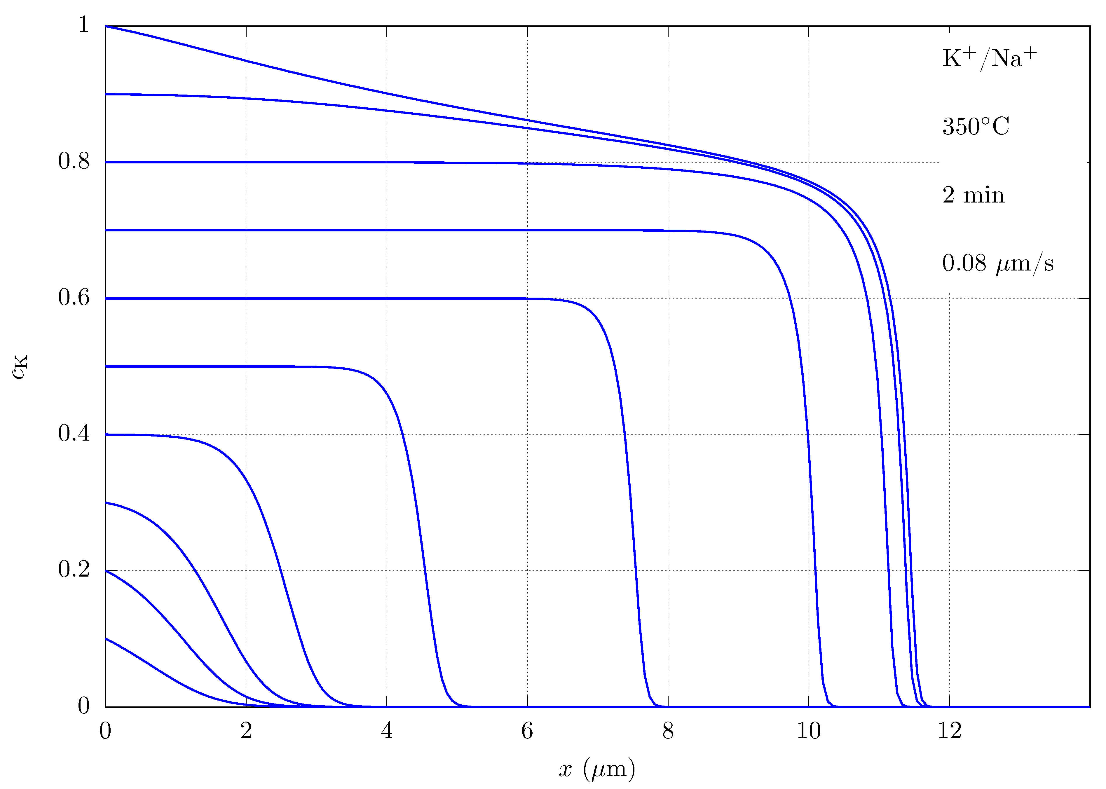
A simulation for field-assisted IE can be seen in Figure 3. For the lowest boundary conditions ( = 0.1–0.3), the exchange was dominated by the diffusive term, and the stable profile was not formed yet. For intermediate values of (0.4–0.8), the stable profile was clearly formed, since the rear region of the profile was flat. Moreover, we can see that the velocity of the front and its slope increased with the boundary condition. Again, these characteristics agreed with the prediction of the basic model. Finally, for = 0.9–1, a new effect appeared. The speed and the slope of the front saturated, while its rear part was no longer flat because the potassium cations were faster here than the sodium ones. Both regimes can be observed in experimental studies [76,77].
4. Future Challenges
Some of the previous assumptions in the modelling of ion exchange in glass are not always valid. For example, the interdiffusion coefficient is reduced during the ion exchange of dopants, which generates compressive stress. This is probably due to a constriction of the interstitial sites [78,79,80]. Another issue is the generalization of the charge neutrality approximation to processes involving the simultaneous diffusion of three species (for example sodium, silver and potassium). Some of such processes were proposed in the past to improve the shape of narrow-channel waveguides [81,82] or, more recently, to obtain both antimicrobial and strengthening properties [10]. In [82], a simplified model was presented by considering that potassium cations are immobile. Unfortunately, little progress has been made in all of these issues in the last few years. Note that modelling of these processes in the MIE framework would require considerable experimental studies to obtain the interdiffusion coefficients. Nevertheless, there are some processes that also require more complete models, but that have recently attracted a great deal of attention due to their remarkable applications. Among them, we highlight: glass poling, electro-diffusion of multivalent metals and the formation/dissolution of silver nanoparticles.
4.1. Glass Poling
Glass poling is the distribution of the electric charges of the glass. This may result in a permanent electric field inside the glass, which can give rise to relevant non-linear effects on light propagation. Applications of glass poling include grating fabrication [83], second-harmonic generation [84] or the fabrication of optical waveguides with profiled electrodes [85]. Glass poling was initially applied to silica glass [86], which contains residual amounts of cations (). It is realized by subjecting the sample to a strong potential difference U (typically, a few kV) at a temperature of about 250–C and, usually, not allowing charged species to enter the glass (“blocking anode”) [87]. Therefore, the field rearranges the cations until a new equilibrium is achieved when the original field inside the glass is cancelled by charges located near the glass surface. That is, the applied field creates a layer, under the anode, a few micrometers thick and depleted of cations. Obviously, charge neutrality is not fulfilled here. Instead, the one-dimensional form of Equations (3) and (10) of the basic model shows that the layer thickness d, in equilibrium, is given by:
This layer is charged and has a high electrical resistivity since its anions are fixed to the glass network. Furthermore, because the field is cancelled in the glass bulk, the applied voltage drops across the depleted layer. Therefore, a very strong field arises, which is independent of the thickness of the substrate. Besides, potentials above ∼1 kV generate structural changes in the layer [88]. Then, if the sample is sharply cooled to room temperature, the distribution of charges becomes frozen. Electric fields inside the silica glass can reach ∼ V/m, which induces a non-linear coefficient (2) ∼ 1 pm/V [89]. However, this process is idealized. In practice, other cations are often involved due to the high applied voltages. One of the possible cations is hydronium () from air water vapour that forms a naturally hydrated layer in the glass. In this situation, called poling with a non-blocking anode, Equation (37) is no longer valid. Instead, a stable profile, such as described in Section 2.4, is formed because hydronium moves slower than sodium. In this case, a partially depleted region is still formed before the electric field increases enough to move the hydronium cations significantly [90]. The charge and the electric field are expected to be at their greatest values when the hydronium layer begins to form. Subsequently, a part of the applied voltage U drops across the hydronium layer [91]. In glasses with high alkali content, the situation is somewhat different, since air cannot provide hydronium at a sufficient rate. Moreover, as is large, d is small (see Equation (37)), and the electric field can become high enough to move other cations such as or [31,92]. Another situation of interest occurs when a BK7 glass, which contains sodium and potassium, is poled. Initially, only sodium cations are removed from the glass surface, as they move faster. Then, the field increases in the charged layer until potassium cations start to move and accumulates behind the sodium ones, filling the empty sites that the latter have just left. Simultaneously, a fully depleted surface layer is formed [92]. Poling of double-alkali glasses, with a non-blocking anode, was also simulated with similar conclusions [93]. One interesting result, which is obtained in high-alkali glasses, is the formation of a waveguide next to the depleted layer, this having non-linear properties. In all the previously cited works about the simulation of glass poling, the authors assumed diffusion coefficients constant, which is only an approximation. The diffusion coefficient in monoalkali glasses depends notably on the alkali content. Therefore, it is expected that the diffusion coefficient in the depleted layer is also different from bulk glass. Therefore, more experimental research on glass poling is still necessary to make clear, on the one hand, the conditions under which the charge neutrality approximation is valid and, on the other hand, whether the MIE or other effects are relevant enough to be considered in the modelling.
4.2. Electro-Diffusion of Multivalent Metals
Monovalent cations as / and / are by far the most used cations in IE processes in glass. However, some successful attempts at doping glass with multivalent cations have also been realized, mainly with transition metals, but also with rare-earths. For example, Gonella et al. obtained , and diffusion profiles in silicate glasses [94,95]; and Cattaruzza et al. introduced cations inside soda-lime glasses [96]. These authors used field-assisted configurations with electric fields up to 400 V/mm, as thermal-assisted IE is not very effective with multivalent ion species. This allowed for penetrations of cations of up to ∼1 m from deposited films. The main utility of glass doping with multivalent transition metals arises from the possibility of converting the glass into an active media. Therefore, optical amplification or waveguide lasers have been demonstrated in erbium-doped glasses [97], and -doped materials have been proposed as both laser gain materials and saturable absorbers for passive Q-switching in IR lasers [98].
The ion exchange with multivalent cations gives rise to concentration-dependent structural changes in the glass matrix. This is due to the local coordination rearrangements, which are produced at the ion sites [99]. In addition, the amount of metal that penetrates into the glass matrix, as well as the shape of the concentration profiles depend strongly on the process parameters. Therefore, the model presented in Section 3, which includes the MIE, should be used in the modelling of such processes. Likewise, when the multivalent cations are introduced into the glass, a region depleted of cations, similar to that observed in poled glasses, is formed. Therefore, the approaches used in the modelling of glass poling could be applied to the present processes. However, little work has been done in these directions, and a comprehensive model of electro-diffusion of multivalent metals is still lacking.
4.3. Formation/Dissolution of Silver Nanoparticles
Metal nanocluster formation following ion exchange can arise if both suitable dopant cations and post-exchange processing techniques are used. Among all dopants, silver stands out for its great diffusivity in glass and its high tendency to form metal clusters [33]. As for the post-exchange techniques, heat treatments (annealing) under different atmospheres [100,101] and (pulsed) laser irradiation [102] are commonly applied. The formation of metal structures can be regarded as a drawback and an advantage. For example, in light waveguiding, metal inhomogeneities must be avoided because they cause a high light absorption. On the contrary, some investigations have found these structures useful for sensing applications, through the surface enhancement of Raman scattering (SERS) [103], for fabricating photonic crystals [104] or, in general, for plasmonic optics [105,106].
Modelling of the formation and dissolution of silver nanoparticles is a very challenging task because the two complex processes compete dynamically. On the one hand, annealing or irradiation promotes silver aggregation and the formation of nanometre-sized clusters while, at the same time, the diffusion and dissolution of silver cations are produced. Therefore, at least three species must be included in the modelling: both exchanging cations and metallic silver. Moreover, this process is often done in gaseous atmospheres, which provide other cations that diffuse into the glass, increasing the number of species to be included in the model. On the other hand, this kind of process is strongly dependent on the cation concentration, so that the MIE should be considered. Finally, not enough experimental studies have been realized until now to characterize the great variety of mechanisms involved in these processes. Some theoretical descriptions of nanoparticle formation under specific post-exchange processing techniques (purely thermal annealing [107] and annealing in hydrogen atmosphere [108]) have been given. Both authors assumed the charge neutrality approximation that, under these processing techniques, is probably fulfilled. However, they did not assess the introduction of the MIE in their models and if that would lead to a better description of the cluster formation. Considerable work, both theoretical and experimental, must be done before having a complete theoretical model of this promising technique.
5. Conclusions
The improvements made in the last few years in the theoretical modelling of ion exchange in glass have contributed to a better understanding of the physical and chemical mechanisms involved in this process. The basic model that has been used for decades only allows for the accurate description of ion exchange problems where the dopant concentration is low. If higher concentrations are present, a model based on the mixed alkali effect must be considered. However, some aspects of this model are still open, because the physics and chemistry involved are not fully understood. On the other hand, a significant progress has been made in the modelling of some IE processes that have attracted much attention in recent years. These processes include glass poling, electro-diffusion of multivalent metals, and the formation/dissolution of silver nanoparticles. All of them have remarkable applications, both scientific, as well as technological.
Funding
This research was funded by Xunta de Galicia, Consellería de Educación, Universidades e FP, Grant GRC Number ED431C2018/11, and Ministerio de Economía, Industria y Competitividad, Gobierno de España, Grant Number AYA2016-78773-C2-2-P, European Regional Development Fund.
Institutional Review Board Statement
Not applicable.
Informed Consent Statement
Not applicable.
Data Availability Statement
Data used in this article data were extracted from Fleming, J.W., Jr.; Day, D.E. Relation of Alkali Mobility and Mechanical Relaxation in Mixed-Alkali Silicate Glasses. J. Am. Ceram. Soc. 1972, 55, 186–192.
Conflicts of Interest
The authors declare no conflict of interest.
Abbreviations
The following abbreviations are used in this manuscript:
| DC | Direct current |
| IE | Ion exchange |
| MIE | Mixed ion effect |
References
- Mazzoldi, P.; Sada, C. A trip in the history and evolution of ion exchange process. Mater. Sci. Eng. B 2008, 149, 112–117. [Google Scholar] [CrossRef]
- Kistler, S.S. Stresses in Glass Produced by Nonuniform Exchange of Monovalent Ions. J. Am. Ceram. Soc. 1962, 45, 59–68. [Google Scholar] [CrossRef]
- Nordberg, M.E.; Mochel, E.L.; Garfinkel, H.M.; Olcott, J.S. Strengthening by Ion Exchange. J. Am. Ceram. Soc. 1964, 47, 215–219. [Google Scholar] [CrossRef]
- Miller, S.E. Integrated Optics: An Introduction. Bell Syst. Tech. J. 1969, 48, 2059–2069. [Google Scholar] [CrossRef]
- Izawa, T.; Nakagone, H. Optical Waveguides Formed by Electrically Induced Migration of Ions in Glass Plates. Appl. Phys. Lett. 1972, 21, 584–586. [Google Scholar] [CrossRef]
- Almeida, R.M.; Marques, A.C. The potential of ion exchange in sol-gel derived photonic materials and structures. Mater. Sci. Eng. B 2008, 149, 118–122. [Google Scholar] [CrossRef]
- Gy, R. Ion exchange for glass strengthening. Mater. Sci. Eng. B 2008, 149, 159–165. [Google Scholar] [CrossRef]
- Karlsson, S.; Jonson, B.; Stålhandske, C. The technology of chemical glass strengthening—A review. Glass Technol. 2010, 51, 41–54. [Google Scholar]
- Varshneya, A.K. Chemical Strengthening of Glass: Lessons Learned and Yet To Be Learned. Int. J. Appl. Glass Sci. 2010, 1, 131–142. [Google Scholar] [CrossRef]
- Guldiren, D.; Erdem, I.; Aydin, S. Influence of silver and potassium ion exchange on physical and mechanical properties of soda lime glass. J. Non-Cryst. Solids 2016, 441, 1–9. [Google Scholar] [CrossRef]
- Macrelli, G.; Varshneya, A.K.; Mauro, J.C. Ion Exchange in Silicate Glasses: Physics of Ion Concentration, Residual Stress, and Refractive Index Profiles. arXiv 2020, arXiv:2002.08016. [Google Scholar]
- Najafi, S.I. (Ed.) Introduction to Glass Integrated Optics; Artech House: Boston, MA, USA; London, UK, 1992. [Google Scholar]
- Opilski, A.; Rogoziński, R.; Gut, K.; Błahut, M.; Opilski, Z. Present state and perspectives involving application of ion exchange in glass. Opto-Electron. Rev. 2000, 8, 117–127. [Google Scholar]
- Honkanen, S.; West, B.R.; Yliniemi, S.; Madasamy, P.; Morrell, M.; Auxier, J.; Schülzgen, A.; Peyghambarian, N.; Carriere, J.; Frantz, J.; et al. Recent advances in ion exchanged glass waveguides and devices. Phys. Chem. Glas. Eur. J. Glass Sci. Andtechnol. Part B 2006, 47, 110–120. [Google Scholar]
- Quaranta, A.; Cattaruzza, E.; Gonella, F. Modelling the ion exchange process in glass: Phenomenological approaches and perspectives. Mater. Sci. Eng. B 2008, 149, 133–139. [Google Scholar] [CrossRef]
- Tervonen, A.; West, B.R.; Honkanen, S. Ion exchanged glass waveguide technology: A review. Opt. Eng. 2011, 50. [Google Scholar] [CrossRef] [Green Version]
- Brusberg, L.; Schröder, H.; Herbst, C.; Frey, C.; Fiebig, C.; Zakharian, A.; Kuchinsky, S.; Liu, X.; Fortusini, D.; Evans, A. High performance ion exchanged integrated waveguides in thin glass for board-level multimode optical interconnects. In Proceedings of the 2015 European Conference on Optical Communication (ECOC), Valencia, Spain, 27 September–1 October 2015; pp. 1–3. [Google Scholar] [CrossRef]
- Wang, F.; Chen, B.; Pun, E.Y.B.; Lin, H. Alkaline aluminum phosphate glasses for thermal ion exchanged optical waveguide. Opt. Mater. 2015, 42, 484–490. [Google Scholar] [CrossRef]
- Salmio, R.P.; Saarinen, J. Graded-Index Diffractive Elements by Thermal Ion Exchange in Glass. Appl. Phys. Lett. 1995, 66, 917–919. [Google Scholar] [CrossRef]
- Singer, W.; Dobler, B.; Schreiber, H.; Brenner, K.H.; Messerschmidt, B. Refractive-index measurement of gradient-index microlenses by diffraction tomography. Appl. Opt. 1996, 35, 2167–2171. [Google Scholar] [CrossRef] [PubMed]
- Montero-Orille, C.; Moreno, V.; Prieto-Blanco, X.; Mateo, E.F.; Ip, E.; Crespo, J.; Liñares, J. Ion exchanged glass binary phase plates for mode-division multiplexing. Appl. Opt. 2013, 52, 2332–2339. [Google Scholar] [CrossRef] [PubMed]
- Rogoziński, R. Ion Exchange in Glass—The Changes of Glass Refraction. Ion Exch. Technol. 2012, 155–190. [Google Scholar] [CrossRef] [Green Version]
- Helfferich, F.; Plesset, M.S. Ion Exchange Kinetics. A Non Linear Diffusion Problem. J. Chem. Phys. 1958, 28, 418–424. [Google Scholar] [CrossRef] [Green Version]
- Abou-el-Leil, M.; Cooper, A.R. Analysis of Field-Assisted Binary Ion Exchange. J. Am. Ceram. Soc. 1979, 62, 390–395. [Google Scholar] [CrossRef]
- Tervonen, A. A General Model for Fabrication Processes of Channel Waveguides by Ion Exchange. J. Appl. Phys. 1990, 67, 2746–2752. [Google Scholar] [CrossRef]
- Cheng, D.; Saarinen, J.; Saarikoski, H.; Tervonen, A. Simulation of Field-assisted Ion exchange for Glass Channel Waveguide Fabrication: Effect of Nonhomogeneous Time-dependent Electric Conductivity. Opt. Commun. 1997, 134, 233–238. [Google Scholar] [CrossRef]
- Fleming, J.W., Jr.; Day, D.E. Relation of Alkali Mobility and Mechanical Relaxation in Mixed-Alkali Silicate Glasses. J. Am. Ceram. Soc. 1972, 55, 186–192. [Google Scholar] [CrossRef]
- Inman, J.M.; Houde-Walter, S.; McIntyre, B.L.; Liao, Z.M.; Parker, R.S.; Simmons, V. Chemical Structure and the Mixed Mobile Ion Effect in Silver-for-Sodium Ion Exchange in Silicate Glass. J. Non-Cryst. Solids 1996, 194, 85–92. [Google Scholar] [CrossRef]
- Lupascu, A.; Kevorkian, A.; Bondet, T.; Saint-André, F.; Persegol, D.; Levy, M. Modeling Ion Exchange in Glass with Concentration Dependent Diffusion Coefficients and Mobilities. Opt. Eng. 1996, 35, 1603–1610. [Google Scholar] [CrossRef]
- Prieto-Blanco, X. Electro-diffusion equations of monovalent cations in glass under charge neutrality approximation for optical waveguide fabrication. Opt. Mater. 2008, 31, 418–428. [Google Scholar] [CrossRef]
- Petrov, M.I.; Lepen’kin, Y.A.; Lipovskii, A.A. Polarization of glass containing fast and slow ions. J. Appl. Phys. 2012, 112, 043101. [Google Scholar] [CrossRef]
- Okorn, B.; Sancho-Parramon, J.; Oljaca, M.; Janicki, V. Metal doping of dielectric thin layers by electric field assisted film dissolution. J. Non-Cryst. Solids 2021, 554, 120584. [Google Scholar] [CrossRef]
- Gonella, F. Silver doping of glasses. Ceram. Int. 2015, 41, 6693–6701. [Google Scholar] [CrossRef]
- Doremus, R.H. Exchange and Diffusion of Ions in Glass. J. Phys. Chem. 1964, 68, 2212–2218. [Google Scholar] [CrossRef]
- Mrozek, P. Numerical modeling of field-assisted Ag+–Na+ ion exchanged channel waveguides using varied explicit space charge density approach. Opt. Appl. 2019, 49. [Google Scholar] [CrossRef]
- Prieto, X.; Srivastava, R.; Liñares, J.; Montero, C. Prediction of Space-Charge Density and Space-Charge Field in Thermally Ion Exchanged Planar Surface Waveguides. Opt. Mater. 1996, 5, 145–151. [Google Scholar] [CrossRef]
- Day, D.E. Mixed Alkali Glasses—Their Properties and Uses. J. Non-Cryst. Solids 1976, 21, 343–372. [Google Scholar] [CrossRef]
- Batchelor, S.; Oven, R.; Ashworth, D.G. Characterization of Electric Field Assisted Diffused Potasium Ion Planar Optical Waveguides. Electron. Lett. 1996, 32, 2082–2083. [Google Scholar] [CrossRef]
- Zheng, W.; Yang, B.; Hao, Y.; Wang, M.; Jiang, X.; Yang, J. Charge-density flux model for electric-field-assisted ion exchange in glass. Opt. Eng. 2011, 50, 1–9. [Google Scholar] [CrossRef]
- Rothmund, V.; Kornfeld, G. Der Basenanstausch im Permutit, I. Z. Anorg. Allg. Chem. 1918, 103, 129. [Google Scholar] [CrossRef]
- Eisenman, G. Cation selective glass electrodes and their mode of operation. Biophys. J. 1962, 2, 259–323. [Google Scholar] [CrossRef] [Green Version]
- Garfinkel, H.M. Ion Exchange Equilibria between Glass and Molten Salts. J. Phys. Chem. 1968, 72, 4175–4181. [Google Scholar] [CrossRef]
- Chludzinski, P.; Ramaswamy, R.V.; Anderson, T.J. Ion Exchange Between Soda-Lime-Silica Glass and Sodium Nitrate-Silver Nitrate Moten Salts. Phys. Chem. Glas. 1987, 28, 169–173. [Google Scholar]
- Crank, J. The Mathematics of Diffusion, 2nd ed.; Oxford Clarenton Press: Oxford, UK, 1979. [Google Scholar]
- Stewart, G.; Laybourn, P.J. Fabrication of Ion Exchanged Optical Waveguides from Dilute Silver Nitrate Melts. IEEE J. Quantum Electron. 1978, QE-14, 930–934. [Google Scholar] [CrossRef]
- Liñares, J.; Prieto, X.; Montero, C. A Novel Refractive Index Profile for Optical Characterization of Nonlinear Diffusion Processes and Planar Waveguides in Glass. Opt. Mater. 1994, 3, 229–236. [Google Scholar] [CrossRef]
- Prieto, X.; Linares, J.; Montero, C. Perturbative method to modelize ion exchange processes: Application to surface waveguides. In Fiber and Integrated Optics; International Society for Optics and Photonics: Bellingham, WA, USA, 1996; Volume 2954, pp. 62–66. [Google Scholar]
- Prieto, X.; Liñares, J. Increasing Resistivity Effects in Field-Assisted Ion Exchange for Planar Optical Waveguide Fabrication. Opt. Lett. 1996, 21, 1–3. [Google Scholar] [CrossRef]
- Anderson, O.L.; Stuart, D.A. Calculation of Activation Energy of Ionic Conductivity in Silica Glasses by Classical Methods. J. Am. Ceram. Soc. 1954, 37, 573–580. [Google Scholar] [CrossRef]
- McVay, G.L.; Day, D.E. Diffusion and Internal Friction in Na-Rb Silicate Glasses. J. Am. Ceram. Soc. 1970, 53, 508–513. [Google Scholar] [CrossRef]
- Hayami, R.; Terai, R. Diffusion of Alkali Ions in Na2O-Cs2O-SiO2 Glasses. Phys. Chem. Glas. 1972, 13, 102–106. [Google Scholar]
- Isard, J. The mixed alkali effect in glass. J. Non-Cryst. Solids 1969, 1, 235–261. [Google Scholar] [CrossRef]
- Terai, R.; Hayami, R. Ionic Diffusion in Glasses. J. Non-Cryst. Solids 1975, 18, 217–264. [Google Scholar] [CrossRef]
- Ingram, M.D. Ionic conductivity in glass. Phys. Chem. Glas. 1987, 28, 215–234. [Google Scholar]
- Araujo, R.J. Interdiffusion in a One-Dimensional Interacting System. J. Non-Cryst. Solids 1993, 152, 70–74. [Google Scholar] [CrossRef]
- Inman, J.M.; Bentley, J.L.; Houde-Walter, S. Modeling Ion Exchanged Glass Photonics: The Modified Quasi-Chemical Diffusion Coefficient. J. Non-Cryst. Solids 1995, 191, 209–215. [Google Scholar] [CrossRef]
- Tomozawa, M. Structure of mixed alkali glasses. J. Non-Cryst. Solids 1996, 196, 280–284. [Google Scholar] [CrossRef]
- Kahnt, H. Ionic transport in glasses. J. Non-Cryst. Solids 1996, 203, 225–231. [Google Scholar] [CrossRef]
- Ngai, K. The dynamics of ions in glasses: Importance of ion–ion interactions. J. Non-Cryst. Solids 2003, 323, 120–126. [Google Scholar] [CrossRef]
- Terai, R. The Mixed Alkali Effect in the Na2O-Cs2O-SiO2 Glasses. J. Non-Cryst. Solids 1971, 6, 121–135. [Google Scholar] [CrossRef]
- Terai, R.; Wakabayashi, H.; Yamanaka, H. Haven ratio in mixed alkali glass. J. Non-Cryst. Solids 1988, 103, 137–142. [Google Scholar] [CrossRef]
- Messerschmidt, B.; Hsieh, C.H.; McIntyre, B.L.; Houde-Walker, S. Ionic Mobility in an Ion Exchanged Silver-Sodium Boroaluminosilicate Glass for Micro-Optics Applications. J. Non-Cryst. Solids 1997, 217, 264–271. [Google Scholar] [CrossRef]
- Lezzi, P.; Tomozawa, M. Enthalpy of mixing of mixed alkali glasses. J. Non-Cryst. Solids 2010, 356, 1439–1446. [Google Scholar] [CrossRef]
- Lezzi, P.; Tomozawa, M. Effect of alumina on enthalpy of mixing of mixed alkali silicate glasses. J. Non-Cryst. Solids 2011, 357, 2086–2092. [Google Scholar] [CrossRef]
- Kouyate, A.; Ahoussou, A.; Yapi, A.; Diabate, D.; Rogez, J.; Trokourey, A. Influence of alkali mixed effect on the mixing enthalpy in 0.75 B2O3 – 0.25 [xNa2O–(1-x)K2O] glass system. Chin. Chem. Lett. 2008, 19, 1252–1255. [Google Scholar] [CrossRef]
- Florian, P.; Vermillion, K.; Grandinetti, P.; Farnan, I.; Stebbins, J. Cation distribution in mixed alkali disilicate glasses. J. Am. Chem. Soc. 1996, 118, 3493–3497. [Google Scholar] [CrossRef]
- Gee, B.; Eckert, H. Cation Distribution in Mixed-Alkali Silicate Glasses. NMR Studies by 23Na-{7Li} and 23Na-{6Li} Spin Echo Double Resonance. J. Phys. Chem. 1996, 100, 3705–3712. [Google Scholar] [CrossRef]
- Ratai, E.; Chan, J.C.; Eckert, H. Local coordination and spatial distribution of cations in mixed-alkali borate glasses. Phys. Chem. Chem. Phys. 2002, 4, 3198–3208. [Google Scholar] [CrossRef]
- Swenson, J.; Matic, A.; Karlsson, C.; Börjesson, L.; Meneghini, C.; Howells, W. Random ion distribution model: A structural approach to the mixed-alkali effect in glasses. Phys. Rev. B 2001, 63, 132202. [Google Scholar] [CrossRef]
- Maass, P.; Bunde, A.; Ingram, M.D. Ion transport anomalies in glasses. Phys. Rev. Lett. 1992, 68, 3064–3067. [Google Scholar] [CrossRef]
- Bunde, A.; Ingram, M.D.; Maass, P. The Dynamic Structure Model for Ion Transport in Glasses. J. Non-Cryst. Solids 1994, 172–174, 1222–1236. [Google Scholar] [CrossRef]
- Bunde, A.; Funke, K.; Ingram, M.D. A unified site relaxation model for ion mobility in glassy materials. Solid State Ionics 1996, 86, 1311–1317. [Google Scholar] [CrossRef]
- Davidson, J.E.; Ingram, M.D.; Bunde, A.; Funke, K. Ion hopping processes and structural relaxation in glassy materials. J. Non-Cryst. Solids 1996, 203, 246–251. [Google Scholar] [CrossRef]
- Murch, G.E. The Nernst-Einstein equation in high-defect-content solids. Philos. Mag. A 1982, 45, 685–692. [Google Scholar] [CrossRef]
- Prieto-Blanco, X.; Montero, C.; Crespo, J.; Barral, D.; Mouriz, D.; Nistal, M.C.; Mateo, E.F.; Moreno, V.; Liñares, J. Hyperbolic interdiffusion for the double alkali effect on index profiles of ion exchanged glass slab optical elements. In Proceedings of the 3rd Congress of the International Commission for Optics, Santiago de Compostela, Spain, 26–29 August 2014. [Google Scholar]
- Prieto Blanco, X. Interferometric characterization and analysis of silver-exchanged glass waveguides buried by electromigration: Slab, channel and slab-sided channel configurations. J. Opt. A Pure Appl. Opt. 2006, 8, 123. [Google Scholar] [CrossRef]
- Sviridov, S.I. Influence of the composition of a molten salt on the field-assisted diffusion of potassium ions in the 20Na2O·80SiO2 glass. Glass Phys. Chem. 2007, 33, 550–555. [Google Scholar] [CrossRef]
- Nogami, M.; Tomozawa, M. Effect of Stress on Water Diffusion in Silica Glass. J. Am. Ceram. Soc. 1984, 67, 151–154. [Google Scholar] [CrossRef]
- Varshneya, A.K.; Dumais, G.A. Influence of Externally Applied Stresses on Kinetics of Ion Exchange in Glass. J. Am. Ceram. Soc. 1985, 68, C-165–C-166. [Google Scholar] [CrossRef]
- Varshneya, A.K. The physics of chemical strengthening of glass: Room for a new view. J. Non-Cryst. Solids 2010, 356, 2289–2294. [Google Scholar] [CrossRef]
- Cooper, A.R. Method for Fabricating Buried Waveguides. EP 0 380 468 A2. Available online: https://data.epo.org/publication-server/document?iDocId=660504&iFormat=0 (accessed on 24 April 2008).
- Tervonen, A.; Honkanen, S. Model for Waveguide Fabrication in Glass by Two-Step Ion Exchange with Ionic Masking. Opt. Lett. 1988, 13, 71–73. [Google Scholar] [CrossRef] [PubMed]
- Lipovskii, A.A.; Rusan, V.V.; Tagantsev, D.K. Imprinting phase/amplitude patterns in glasses with thermal poling. Solid State Ionics 2010, 181, 849–855. [Google Scholar] [CrossRef]
- Garcia, F.C.; Carvalho, I.C.S.; Hering, E.; Margulis, W.; Lesche, B. Inducing a large second-order optical nonlinearity in soft glasses by poling. Appl. Phys. Lett. 1998, 72, 3252–3254. [Google Scholar] [CrossRef]
- Zhurikhina, V.; Sadrieva, Z.; Lipovskii, A. Single-mode channel optical waveguides formed by the glass poling. Optik 2017, 137, 203–208. [Google Scholar] [CrossRef]
- Myers, R.A.; Mukherjee, N.; Brueck, S.R.J. Large second-order nonlinearity in poled fused silica. Opt. Lett. 1991, 16, 1732–1734. [Google Scholar] [CrossRef]
- Fleming, S.C.; An, H. Poled glasses and poled fibre devices. J. Ceram. Soc. Jpn. 2008, 116, 1007–1023. [Google Scholar] [CrossRef] [Green Version]
- An, H.; Fleming, S. Near-anode phase separation in thermally poled soda lime glass. Appl. Phys. Lett. 2006, 88, 181106. [Google Scholar] [CrossRef]
- Kudlinski, A.; Quiquempois, Y.; Martinelli, G. Modeling of the χ(2) susceptibility time-evolution in thermally poled fused silica. Opt. Express 2005, 13, 8015–8024. [Google Scholar] [CrossRef]
- Petrov, M.I.; Omelchenko, A.V.; Lipovskii, A.A. Electric field and spatial charge formation in glasses and glassy nanocomposites. J. Appl. Phys. 2011, 109, 094108. [Google Scholar] [CrossRef]
- Lipovskii, A.; Omelchenko, A.; Petrov, M. Modeling charge transfer dynamics and electric field distribution in glasses during poling and electrostimulated diffusion. Tech. Phys. Lett. 2010, 36, 1028–1031. [Google Scholar] [CrossRef]
- Brennand, A.L.R.; Wilkinson, J.S. Planar waveguides in multicomponent glasses fabricated by field-driven differential drift of cations. Opt. Lett. 2002, 27, 906–908. [Google Scholar] [CrossRef] [PubMed] [Green Version]
- Oven, R. Analytical model of electric field assisted ion diffusion into glass containing two indigenous mobile species, with application to poling. J. Non-Cryst. Solids 2021, 553, 120476. [Google Scholar] [CrossRef]
- Gonella, F.; Cattaruzza, E.; Quaranta, A.; Ali, S.; Argiolas, N.; Sada, C. Diffusion behavior of transition metals in field-assisted ion exchanged glasses. Solid State Ionics 2006, 177, 3151–3155. [Google Scholar] [CrossRef] [Green Version]
- Cattaruzza, E.; Battaglin, G.; Gonella, F.; Quaranta, A.; Mariotto, G.; Sada, C.; Ali, S. Chromium doping of silicate glasses by field-assisted solid-state ion exchange. J. Non-Cryst. Solids 2011, 357, 1846–1850. [Google Scholar] [CrossRef]
- Cattaruzza, E.; Gonella, F.; Peruzzo, G.; Quaranta, A.; Sada, C.; Trave, E. Field-assisted ion diffusion in dielectric matrices: Er3+ in silicate glass. Mater. Sci. Eng. B 2008, 146, 163–166. [Google Scholar] [CrossRef]
- Kenyon, A. Recent developments in rare-earth doped materials for optoelectronics. Prog. Quantum Electron. 2002, 26, 225–284. [Google Scholar] [CrossRef]
- Kalisky, Y. Cr4+-doped crystals: Their use as lasers and passive Q-switches. Prog. Quantum Electron. 2004, 28, 249–303. [Google Scholar] [CrossRef]
- Thévenin-Annequin, C.; Levy, M.; Pagnier, T. Electrochemical study of the silver-sodium substitution in a borosilicate glass. Solid State Ionics 1995, 80, 175–179. [Google Scholar] [CrossRef]
- Marchi, G.D.; Caccavale, F.; Gonella, F.; Mattei, G.; Mazzoldi, P.; Battaglin, G.; Quaranta, A. Silver nanoclusters formation in ion exchanged waveguides by annealing in hydrogen atmosphere. Appl. Phys. A 1996, 63, 403–407. [Google Scholar] [CrossRef]
- Mohr, C.; Dubiel, M.; Hofmeister, H. Formation of silver particles and periodic precipitate layers in silicate glass induced by thermally assisted hydrogen permeation. J. Phys. Condens. Matter 2000, 13, 525–536. [Google Scholar] [CrossRef] [Green Version]
- Cattaruzza, E.; Mardegan, M.; Trave, E.; Battaglin, G.; Calvelli, P.; Enrichi, F.; Gonella, F. Modifications in silver-doped silicate glasses induced by ns laser beams. Appl. Surf. Sci. 2011, 257, 5434–5438. [Google Scholar] [CrossRef]
- Chen, Y.; Karvonen, L.; Säynätjoki, A.; Ye, C.; Tervonen, A.; Honkanen, S. Ag nanoparticles embedded in glass by two-step ion exchange and their SERS application. Opt. Mater. Express 2011, 1, 164–172. [Google Scholar] [CrossRef]
- Kaganovsky, Y.S.; Antonov, I.; Rosenbluh, M.; Ihlemann, J.; Lipovskii, A. Two- and Three-Dimensional Photonic Crystals Produced by Pulsed Laser Irradiation in Silver-Doped Glass. Functional Nanomaterials for Optoelectronics and other Applications. In Solid State Phenomena; Trans Tech Publications Ltd.: Stafa-Zurich, Switzerland, 2004; Volume 99, pp. 65–72. [Google Scholar] [CrossRef]
- Kumar, P.; Mathpal, M.C.; Tripathi, A.K.; Prakash, J.; Agarwal, A.; Ahmad, M.M.; Swart, H.C. Plasmonic resonance of Ag nanoclusters diffused in soda-lime glasses. Phys. Chem. Chem. Phys. 2015, 17, 8596–8603. [Google Scholar] [CrossRef]
- Warren, S.; Thimsen, E. Plasmonic solar water splitting. Energy Environ. Sci. 2012, 5, 5133–5146. [Google Scholar] [CrossRef]
- Berger, A. Concentration and size depth profile of colloidal silver particles in glass surfaces produced by sodium-silver ion exchange. J. Non-Cryst. Solids 1992, 151, 88–94. [Google Scholar] [CrossRef]
- Redkov, A.; Zhurikhina, V.; Lipovskii, A. Formation and self-arrangement of silver nanoparticles in glass via annealing in hydrogen: The model. J. Non-Cryst. Solids 2013, 376, 152–157. [Google Scholar] [CrossRef]
Figure 1.
Self-diffusion and interdiffusion coefficients, as well as mobility, calculated from experimental data obtained by radiative tracers [27], as a function of the normalized concentration for / IE. The Haven ratio was ignored. (a) Basic model—Equations (5) and (9)—which assumes that the self-diffusion coefficients remain constant with the cation mole fraction. (b) The same functions taking into account the MIE. Quadratic polynomials in were fitted to the logarithms of the experimental self-diffusion coefficients and then used to calculate the rest of the functions through the definitions (35) and (34). Note the difference between and , which are the expected interdiffusion coefficients when the interaction among cations or the ideal mixture is assumed, respectively.
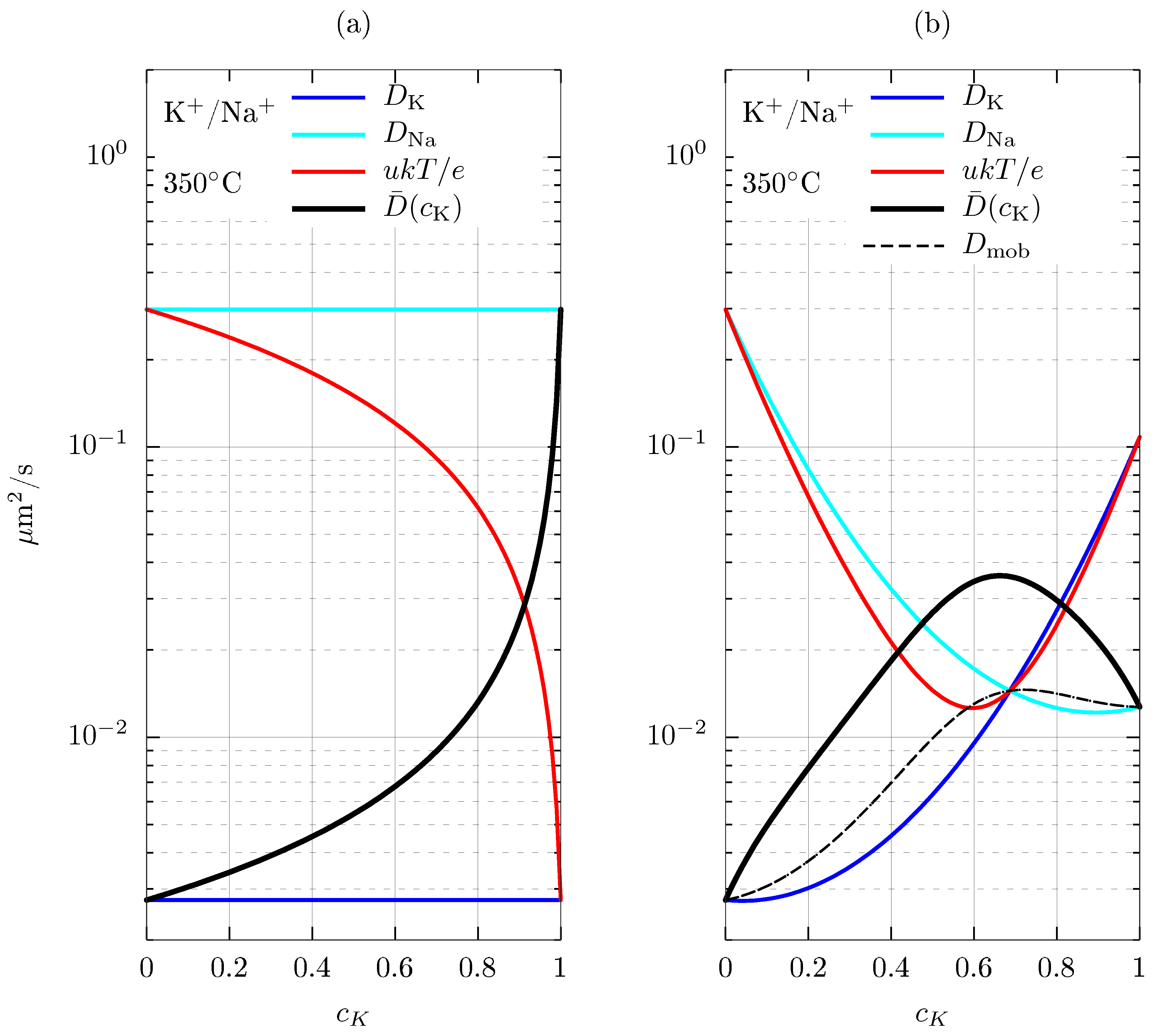
Figure 2.
Simulation of molar fraction profiles as a function of depth for a thermal IE by taking into account the MIE. Equation (31) was solved for and the boundary conditions = 0.2, 0.4, 0.6, 0.8 and 1. The interdiffusion coefficient of Figure 1b was used.
Figure 2.
Simulation of molar fraction profiles as a function of depth for a thermal IE by taking into account the MIE. Equation (31) was solved for and the boundary conditions = 0.2, 0.4, 0.6, 0.8 and 1. The interdiffusion coefficient of Figure 1b was used.
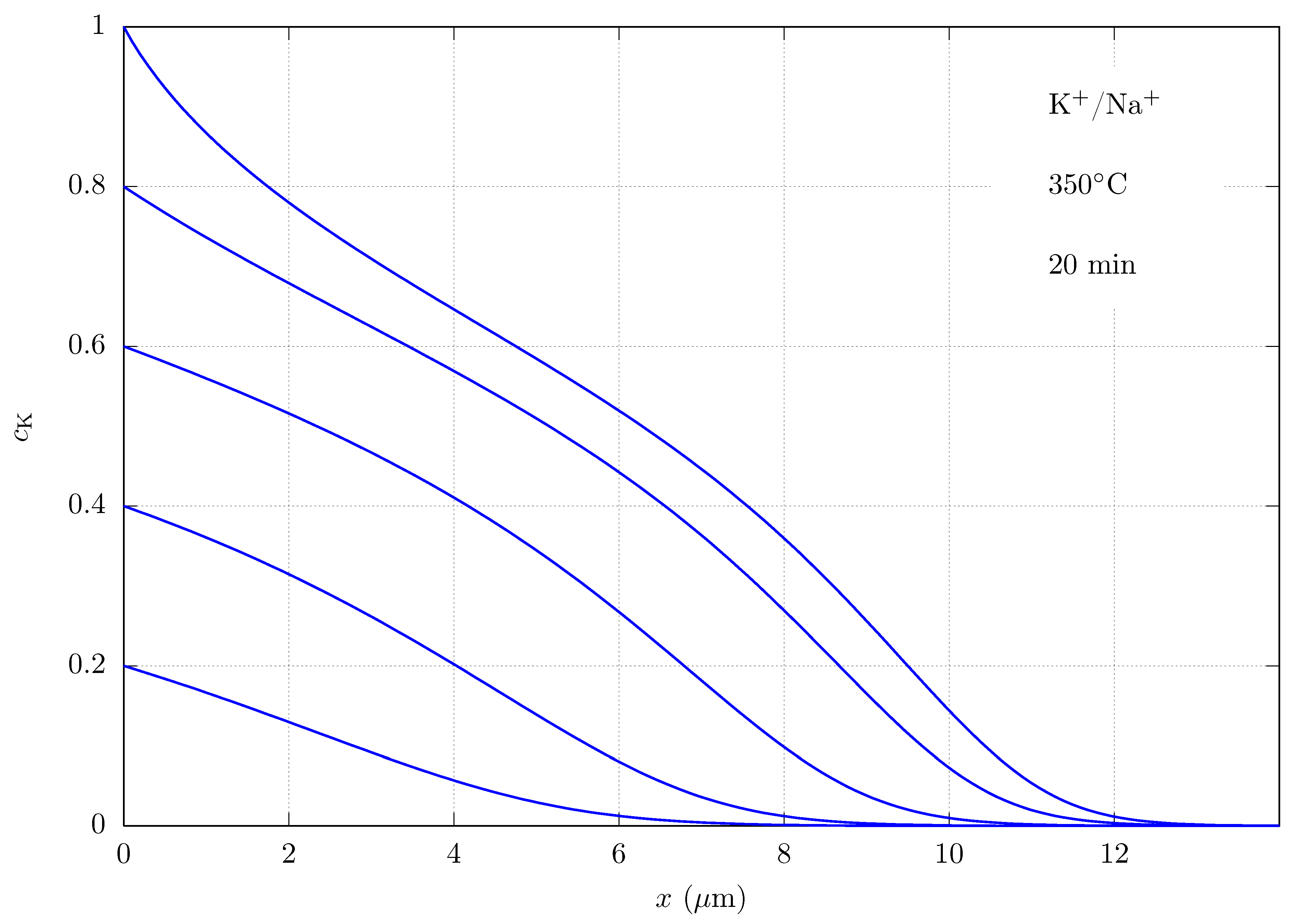
Figure 3.
Simulation similar to that in Figure 2, but for a field-assisted IE with = 80 nm/s.
Figure 3.
Simulation similar to that in Figure 2, but for a field-assisted IE with = 80 nm/s.

Table 1.
Complete formulation of the IE problem (equations and boundary conditions), for the most common IE processes, in terms of the normalized concentration of dopant cations and the total flux density ; is a unit vector perpendicular to the sample surface, and C is a constant, which mainly depends on the dopant concentration in the salt.
| Equations | ||
| Salt | ||
| Film | ||
| Mask/Air | ||
| with | ||
Table 2.
Complete formulation of the IE problem (equations and boundary conditions), for the most common IE processes, in terms of the normalized concentration of dopant cations and an effective electric potential ; is a unit vector perpendicular to the sample surface, and C and F are constants.
Table 2.
Complete formulation of the IE problem (equations and boundary conditions), for the most common IE processes, in terms of the normalized concentration of dopant cations and an effective electric potential ; is a unit vector perpendicular to the sample surface, and C and F are constants.
| Equations | ||
| Salt | ||
| Film | ||
| Mask/Air | ||
| with | ||
Publisher’s Note: MDPI stays neutral with regard to jurisdictional claims in published maps and institutional affiliations. |
© 2021 by the authors. Licensee MDPI, Basel, Switzerland. This article is an open access article distributed under the terms and conditions of the Creative Commons Attribution (CC BY) license (https://creativecommons.org/licenses/by/4.0/).
Share and Cite
MDPI and ACS Style
Prieto-Blanco, X.; Montero-Orille, C. Theoretical Modelling of Ion Exchange Processes in Glass: Advances and Challenges. Appl. Sci. 2021, 11, 5070. https://doi.org/10.3390/app11115070
AMA Style
Prieto-Blanco X, Montero-Orille C. Theoretical Modelling of Ion Exchange Processes in Glass: Advances and Challenges. Applied Sciences. 2021; 11(11):5070. https://doi.org/10.3390/app11115070
Chicago/Turabian StylePrieto-Blanco, Xesús, and Carlos Montero-Orille. 2021. "Theoretical Modelling of Ion Exchange Processes in Glass: Advances and Challenges" Applied Sciences 11, no. 11: 5070. https://doi.org/10.3390/app11115070
Note that from the first issue of 2016, this journal uses article numbers instead of page numbers. See further details here.