
Remaining Useful Life Prediction of Cutting Tools Using an Inverse Gaussian Process Model


Abstract
:1. Introduction
2. Methods
2.1. Performance Degradation Modeling Based on Inverse Gaussian Process
2.2. Remaining Useful Life Evaluation Model
2.3. Parameter Estimation Based on Expectation–Maximization (EM)
3. Example Study
3.1. Simulation
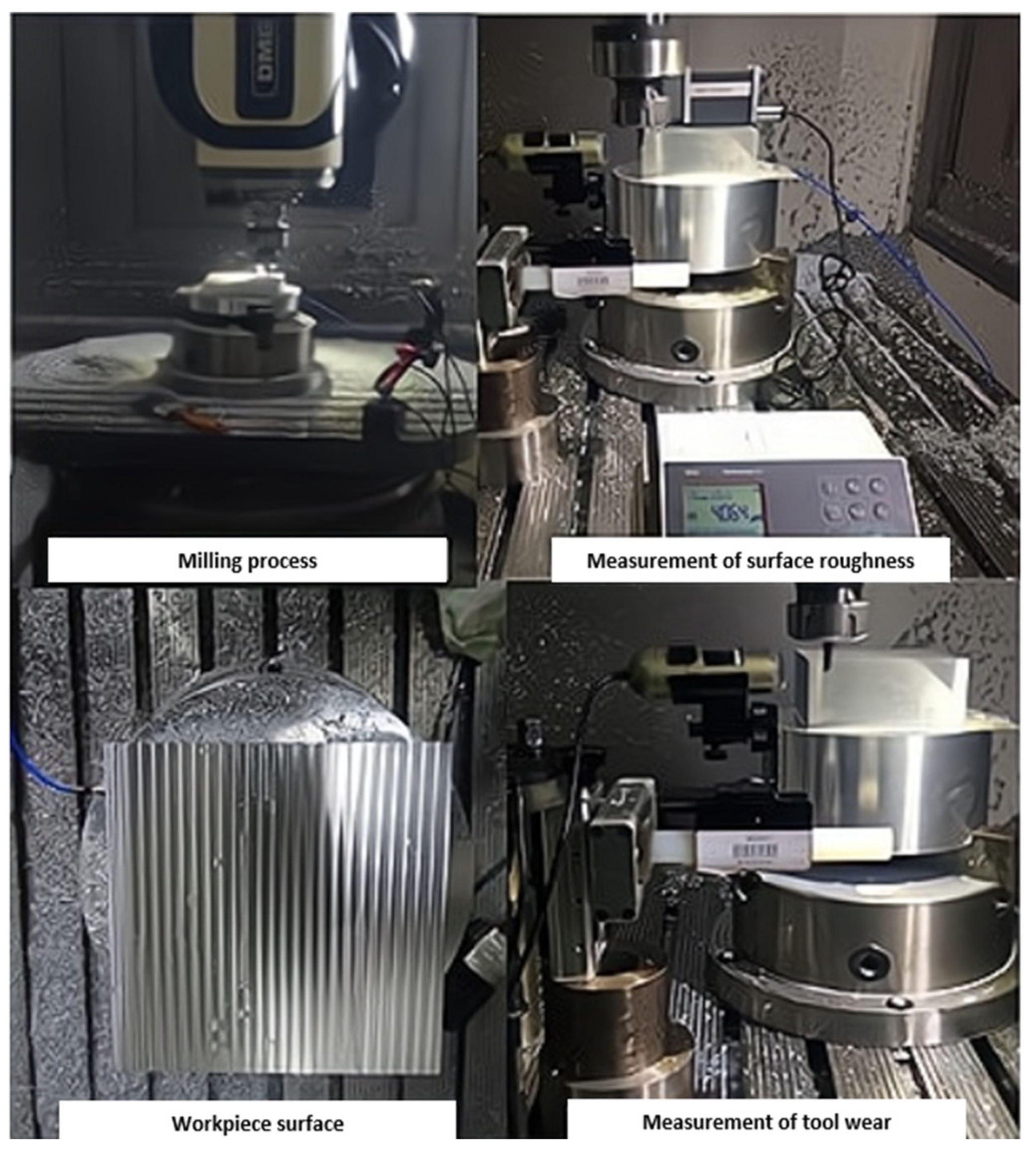
3.2. Experiment
3.3. Comparation of the RUL Predictive Model
4. Conclusions
- 1.
- An IG process model with a variable drift coefficient was used to characterize the degradation of the tool wearing process subjected to individual heterogeneity in dynamic working environments;
- 2.
- The surface roughness requirement was linked to a random threshold for the wearing of the cutting tool, and the RUL prediction method was developed based on the proposed degradation model with a random failure threshold.
- 3.
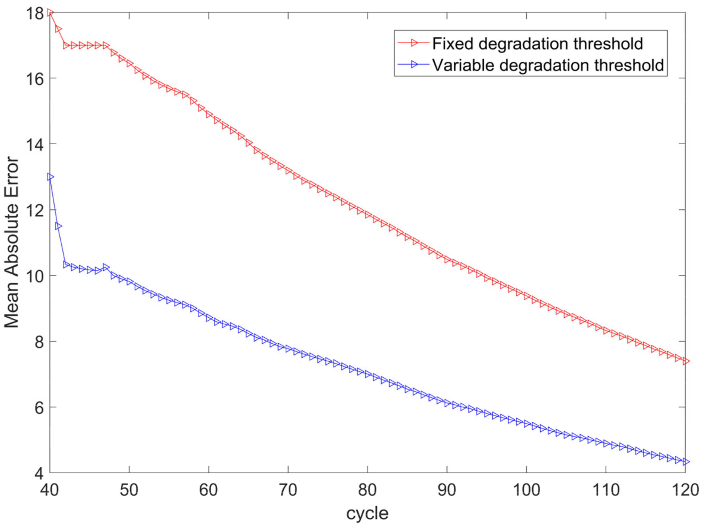
- Finally, the applicability and effectiveness of the proposed method was validated using the wearing data of cutting tools in a milling experiment; the MAE was 4.33.
Author Contributions
Funding
Conflicts of Interest
Abbreviation
| RUL | remaining useful life | |
| IG | inverse Gaussian | |
| EM | expectation-maximization | |
| probability density function | ||
| CDF | cumulative distribution function | |
| Ra | surface roughness | |
| Y(t) | degradation process with a simple IG process model | |
| μ | degeneration rate of Y(t) | |
| λ | fluctuation coefficient of Y(t) | |
| Λ(t) | monotone increasing function of Y(t) | |
| ω | failure threshold | |
| T | failure time | |
| Tr | residual life | |
| FT(t) | CDF of T | |
| fT(t) | PDF of T | |
| P(∙) | probability of an event | |
| E(∙) | expectation operator | |
| N(a, b) | uniform distribution with boundary [a, b] | |
| Φ(∙) | CDF of standard normal distribution | |
| distribution of Parameter 1/μ | ||
| derivative function of Λ(t) | ||
| tk | kth measurement time | |
| Rk | RUL corresponding to the equipment at the current measurement time tk | |
| Y0:k | historical degenerate dataset from start time t0 to time tk. | |
| Λ(t) at the measurement time tk | ||
| Λ(t) at the initial time | ||
| FTr(t) | CDF of Tr | |
| fTr(t) | PDF of Tr | |
| FRk(rk) | CDF of Rk at tk | |
| fRk(rk) | PDF of Rk at tk | |
| degradation value at time tk | ||
| degradation increment | ||
| j | iteration times | |
| θ | estimated parameters θ= (αμ, σμ−2, λ) | |
| is the parameter θ at time tk after j iterations | ||
| posterior distribution of 1/μk at tk | ||
| joint log-likelihood function for observed events, Y0:k and 1/μk | ||
| prior distribution of 1/μk at tk | ||
| complete log-likelihood function of {Y0:k,} | ||
| joint density function for observed events,Y0:k, 1/μ, and θ | ||
| conditional probability density, with the parameter 1/μ and parameter θ are known | ||
| joint density function for observed events,1/μ and θ | ||
| optimal parameters | ||
| MAE | mean absolute error | |
| predicted RUL at the i cycle | ||
| actual RUL at the i cycle | ||
References
- Zhu, K.; Liu, T. Online tool wear monitoring via hidden semi-markov model with dependent durations. IEEE Trans. Ind. Inform. 2018, 14, 69–78. [Google Scholar] [CrossRef]
- Wang, M.; Wang, J. CHMM for tool condition monitoring and remaining useful life prediction. Int. J. Adv. Manuf. Technol. 2012, 59, 463–471. [Google Scholar] [CrossRef]
- Wei, W.; Hu, J.; Zhang, J. Prognostics of machine health condition using an improved ARIMA-based prediction method. In Proceedings of the IEEE Conference on Industrial Electronics and Applications, Harbin, China, 23–25 May 2007; pp. 1062–1067. [Google Scholar] [CrossRef] [Green Version]
- Zheng, X.; Fang, H. An integrated unscented kalman filter and relevance vector regression approach for lithium-ion battery remaining useful life and short-term capacity prediction. Reliab. Eng. Syst. Saf. 2015, 144, 74–82. [Google Scholar] [CrossRef]
- Singleton, R.K.; Strangas, E.G.; Aviyente, S. Extended kalman filtering for remaining-useful-life estimation of bearings. Ind. Electron. IEEE Trans. 2015, 62, 1781–1790. [Google Scholar] [CrossRef]
- Qiang, M.; Lei, X.; Cui, H.; Liang, W.; Pecht, M. Remaining useful life prediction of lithium-ion battery with unscented particle filter technique. Microelectron. Reliab. 2013, 53, 805–810. [Google Scholar] [CrossRef]
- Qian, Y.; Yan, R. Remaining useful life prediction of rolling bearings using an enhanced particle filter. IEEE Trans. Instrum. Meas. 2015, 64, 2696–2707. [Google Scholar] [CrossRef]
- Peng, W.; Gao, R.X. Adaptive resampling-based particle filtering for tool life prediction. J. Manuf. Syst. 2015, 37, 528–534. [Google Scholar] [CrossRef]
- Wang, J.; Peng, W.; Gao, R.X. Enhanced particle filter for tool wear prediction. J. Manuf. Syst. 2015, 36, 35–45. [Google Scholar] [CrossRef]
- Karam, S.; Centobelli, P.; D’addona, D.M.; Teti, R. Online prediction of cutting tool life in turning via cognitive decision making. Procedia CIRP 2016, 41, 927–932. [Google Scholar] [CrossRef]
- Marani, M.; Zeinali, M.; Kouam, J.; Songmene, V.; Mechefske, C.K. Prediction of cutting tool wear during a turning process using artificial intelligence techniques. Int. J. Adv. Manuf. Technol. 2020, 111, 505–515. [Google Scholar] [CrossRef]
- Marani, M.; Zeinali, M.; Songmene, V.; Mechefske, C.K. Tool wear prediction in high-speed turning of a steel alloy using long short-term memory modelling. Measurement 2021, 177, 109329. [Google Scholar] [CrossRef]
- Benkedjouh, T.; Medjaher, K.; Zerhouni, N.; Rechak, S. Health assessment and life prediction of cutting tools based on support vector regression. J. Intell. Manuf. 2015, 26, 213–223. [Google Scholar] [CrossRef] [Green Version]
- Sun, C.; Ma, M.; Zhao, Z.; Tian, S.; Yan, R.; Chen, X. Deep transfer learning based on sparse auto-encoder for remaining useful life prediction of tool in manufacturing. IEEE Trans. Ind. Inform. 2018, 15, 2416–2425. [Google Scholar] [CrossRef]
- Zhu, J.; Chen, N.; Peng, W. Estimation of bearing remaining useful life based on multiscale convolutional neural network. Ind. Electron. IEEE Trans. 2019, 66, 3208–3216. [Google Scholar] [CrossRef]
- Si, X.S.; Wang, W.; Hu, C.H.; Chen, M.-Y.; Zhou, D.-H. A Wiener-process-based degradation model with a recursive filter algorithm for remaining useful life estimation. Mech. Syst. Signal Process. 2013, 35, 219–237. [Google Scholar] [CrossRef]
- Zhai, Q.; Ye, Z.-S. Degradation in common dynamic environments. Technometrics 2018, 60, 461–471. [Google Scholar] [CrossRef]
- Sun, H.; Cao, D.; Zhao, Z.; Kang, X. A hybrid approach to cutting tool remaining useful life prediction based on the wiener process. IEEE Trans. Reliab. 2018, 67, 1294–1303. [Google Scholar] [CrossRef]
- Xu, W.; Wang, W. An adaptive gamma process based model for residual useful life prediction. In Proceedings of the IEEE 2012 Prognostics and System Health Management Conference, Beijing, China, 1–4 May 2012. [Google Scholar] [CrossRef]
- Pan, D.; Liu, J.-B.; Cao, J. Remaining useful life estimation using an inverse Gaussian degradation model. Neurocomputing 2016, 185, 64–72. [Google Scholar] [CrossRef] [Green Version]
- Ma, Z.; Wang, S.; Liao, H.; Zhang, C. Engineering-driven performance degradation analysis of hydraulic piston pump based on the inverse Gaussian process. Qual. Reliab. Eng. 2019, 35, 2278–2296. [Google Scholar] [CrossRef]
- Mikołajczyk, T.; Nowicki, K.; Bustillo, A.; Pimenov, D.Y. Predicting tool life in turning operations using neural networks and image processing. Mech. Syst. Signal Process. 2018, 104, 503–513. [Google Scholar] [CrossRef]
- Guo, J.; Zheng, H.; Li, B.; Guo-Zhong, F. A bayesian approach for degradation analysis with individual differences. IEEE Access 2019, 7, 175033–175040. [Google Scholar] [CrossRef]
- Lu, C.J.; Meeker, W.O. Using degradation measures to estimate a time-to-failure distribution. Technometrics 1993, 35, 161–174. [Google Scholar] [CrossRef]
- Peng, C.Y.; Tseng, S.T. Mis-specification analysis of linear degradation models. IEEE Trans. Reliab. 2009, 58, 444–455. [Google Scholar] [CrossRef]
- Chen, X.; Sun, X.; Si, X.; Li, G. Remaining useful life prediction based on an adaptive inverse gaussian degradation process with measurement errors. IEEE Access. 2020, 8, 3498–3510. [Google Scholar] [CrossRef]
- Ye, Z.-S.; Chen, N. The inverse Gaussian process as a degradation model. Technometrics 2014, 56, 302–311. [Google Scholar] [CrossRef]
- Savsar, M. Effects of degraded operation modes on reliability and performance of manufacturing cells. Int. J. Ind. Syst. Eng. 2012, 11, 189–204. [Google Scholar] [CrossRef]
- Bustillo, A.; Pimenov, D.Y.; Matuszewski, M.; Mikolajczyk, T. Using artificial intelligence models for the prediction of surface wear based on surface isotropy levels. Robot. Comput. Integr. Manuf. 2018, 53, 215–227. [Google Scholar] [CrossRef]
- Debnath, S.; Reddy, M.M. Influence of cutting fluid conditions and cutting parameters on surface roughness and tool wear in turning process using Taguchi method. Measurement 2016, 78, 111–119. [Google Scholar] [CrossRef]
- Kull Neto, H.; Diniz, A.E. Tool life and surface roughness in the milling of curved hardened-steel surfaces. Int. J. Adv. Manuf. Technol. 2016, 87, 2983–2995. [Google Scholar] [CrossRef]
- Nieslony, P.; Krolczyk, G.M. Surface quality and topographic inspection of variable compliance part after precise turning. Appl. Surf. Sci. 2018, 434, 91–101. [Google Scholar] [CrossRef]
- Bulaha, N. Analysis of service properties of cylindrically ground surfaces, using standard ISO 25178-2:2012 surface texture parameters. Environ. Technol. Resour. Proc. Int. Sci. Pr. Conf. 2015, 1, 16–21. [Google Scholar] [CrossRef]
- Zhang, J.Z.; Chen, J.C. The development of an in-process surface roughness adaptive control system in turning operations. J. Intell. Manuf. 2007, 18, 301–311. [Google Scholar] [CrossRef]
- Abellan, J.V.; Subirón, F.R. A review of machining monitoring systems based on artificial intelligence process models. Int. J. Adv. Manuf. Technol. 2010, 47, 237–257. [Google Scholar] [CrossRef]
- Ye, Z.; Chen, L.; Tang, L.; Xie, M. Accelerated degradation test planning using the inverse Gaussian process. IEEE Trans. Reliab. 2014, 63, 750–763. [Google Scholar] [CrossRef]
- Chien, Y.-P. Inverse gaussian processes with random effects and explanatory variables for degradation data. Technometrics 2015, 57, 100–111. [Google Scholar] [CrossRef]
- Peng, W.; Li, Y.F.; Yang, Y.J.; Huang, H.-Z.; Zuo, M.J. Inverse Gaussian process models for degradation analysis: A Bayesian perspective. Reliab. Eng. Syst. Saf. 2014, 130, 175–189. [Google Scholar] [CrossRef]
- Si, X.S.; Zhou, D. A generalized result for degradation model-based reliability estimation. IEEE Trans. Autom. Sci. Eng. 2014, 11, 632–637. [Google Scholar] [CrossRef]
- Zhai, Q.; Ye, Z. RUL prediction of deteriorating products using an adaptive wiener process model. IEEE Trans. Ind. Inform. 2017, 13, 2911–2921. [Google Scholar] [CrossRef]
- Zhang, Z.; Si, X.; Hu, C.; Lei, Y. Degradation data analysis and remaining useful life estimation: A review on wiener-process-based methods. Eur. J. Oper. Res. 2018, 271, 775–796. [Google Scholar] [CrossRef]


| Material | Chemical Composition % | ||||||||||
|---|---|---|---|---|---|---|---|---|---|---|---|
| 7109 | Si | Fe | Cu | Mn | Mg | Cr | Zn | Zr | Co | O | Ti |
| 0.1 | 0.15 | 0.1 | 0.05 | 2.4 | 0.06 | 6.2 | 0.15 | 0.2 | 0.05 | 0.1 | |
| Grade | Helical Angle | Number of Teeth | Diameter | Over Length | Edge Length | Cutting Edge Diameter | Material |
|---|---|---|---|---|---|---|---|
| ZCC.CT (China) | 55° | 3 | 6 mm | 50 mm | 12 mm | 4 mm | Cemented Carbide |
| Model | Prediction Distribution Falls within 1 ± 0.1 of True RUL |
|---|---|
| IG process model | 72% |
| Particle filtering model | 60% |
Publisher’s Note: MDPI stays neutral with regard to jurisdictional claims in published maps and institutional affiliations. |
© 2021 by the authors. Licensee MDPI, Basel, Switzerland. This article is an open access article distributed under the terms and conditions of the Creative Commons Attribution (CC BY) license (https://creativecommons.org/licenses/by/4.0/).
Share and Cite
Huang, Y.; Lu, Z.; Dai, W.; Zhang, W.; Wang, B. Remaining Useful Life Prediction of Cutting Tools Using an Inverse Gaussian Process Model. Appl. Sci. 2021, 11, 5011. https://doi.org/10.3390/app11115011
Huang Y, Lu Z, Dai W, Zhang W, Wang B. Remaining Useful Life Prediction of Cutting Tools Using an Inverse Gaussian Process Model. Applied Sciences. 2021; 11(11):5011. https://doi.org/10.3390/app11115011
Chicago/Turabian StyleHuang, Yuanxing, Zhiyuan Lu, Wei Dai, Weifang Zhang, and Bin Wang. 2021. "Remaining Useful Life Prediction of Cutting Tools Using an Inverse Gaussian Process Model" Applied Sciences 11, no. 11: 5011. https://doi.org/10.3390/app11115011
APA StyleHuang, Y., Lu, Z., Dai, W., Zhang, W., & Wang, B. (2021). Remaining Useful Life Prediction of Cutting Tools Using an Inverse Gaussian Process Model. Applied Sciences, 11(11), 5011. https://doi.org/10.3390/app11115011