Multi-Sensor Fusion Positioning Method Based on Batch Inverse Covariance Intersection and IMM

Abstract

For mass application positioning demands, the current single positioning sensor cannot provide reliable and accurate positioning. Herein, we present batch inverse covariance intersection (BICI) and BICI with interacting multiple model (BICI-IMM) multi-sensor fusion positioning methods, which are based on the batch form of the sequential inverse covariance intersection (SICI) fusion method. Meanwhile, it is proved that the BICI is robust. Compared with SICI, BICI-IMM reduces estimation error variance of the motion model and has less conservativeness. The BICI-IMM algorithm improves the accuracy of local filtering by interacting with multiple models and realizes global fusion estimation based on BICI. The validity of the BICI and BICI-IMM algorithm are demonstrated by two simulations and experiments in the open and semi-open scenes, and its positioning accuracy relations are shown. In addition, it is demonstrated that the BICI-IMM algorithm can improve the positioning accuracy in the actual scenes.

1. Introduction

With the advent of the era of Internet of everything, indoor and outdoor positioning information with high accuracy, high reliability, large capacity and low delay has became indispensable, which is vital for intelligent robots, unmanned driving and other unmanned platforms. The sensor positioning algorithm usually adopts time of arrival (ToA), difference of arrival (TDoA), angle of arrival (AoA), direction of arrival (DoA), frequency difference of arrival (FDoA), time of flight (ToF) and received signal strength indication (RSSI) [1,2,3,4]. The sensor measurement for positioning comes from global navigation satellite systems (GNSS), Wi-Fi [5], RFID [6], Bluetooth [7], vision [8], UWB [9], etc. GNSS has been widely applied in various scenes; unfortunately, it is difficult to position in indoor and canyon environments due to its inherent fragility [10]. Although many other sensors are available, they have are defects such as a small coverage and high cost. Therefore, a single sensor is hard to position with high precision, high reliability and availability in challenging scenarios.

Compared with a single sensor, multiple-sensor fusion can improve coverage, estimation accuracy and reliability because it combines the advantages of each information source. Multi-sensor fusion algorithms usually adopt Kalman filtering, support vector machine (SVM), Bayesian inference, Dempster–Shafer theory of evidence and artificial neural networks (ANN) [11]. The Kalman filter is frequently chosen for real-time fusion positioning in robotic applications because of its high computational efficiency. Multi-sensor fusion methods are mainly divided into centralized and distributed methods, where the difference is whether the original measurements are capable of direct fusion. The former can obtain a global optimal state estimation by expanded measurement equations and covariance matrix, but there are some drawbacks such as its computational complexity, fault tolerance and flexibility. The latter accesses a global optimal estimation from local filters. Distributed fusion methods include diagonal matrix, scalar weighted fusion and minimum covariance determinant (MCD) [12,13], etc., which need covariance among local filters. However, it is difficult to obtain covariance in the actual scene. For the multi-sensor fusion estimation problem with an unknown covariance, Julier and Uhlmann proposed a covariance intersection (CI) method, which uses the conservative error variance upper bound to avoid covariance calculation [14]. The accuracy of fusion positioning algorithms of batch covariance intersection (BCI) [15], sequential covariance intersection (SCI) [16] and parallel covariance intersection (PCI) [17] is limited because of the more conservative CI method. Sijs et al. showed an ellipsoid intersection (EI) algorithm, which used a common error to model the unknown correlation. The estimation accuracy of EI is better than CI [18]. However, EI has a worse robustness of fusion estimation because of its inconsistent estimation [19,20]. Noack et al. changed the parameters of EI to ensure consistency, and proposed an inverse covariance intersection (ICI) method [21]. Based on the ICI method, Chen et al. designed a sequential inverse covariance intersection (SICI) fusion method for packet dropouts, which solved the fusion problem with unknown covariances and had good estimation performance [22]. Tang et al. showed an information geometric fusion method [23], which adopted the information center of local posterior densities and had a high computational burden.

The current research on fusion positioning with an unknown motion model mainly focuses on model uncertainty and has precise noise variance. However, sensor noise variance is time-varying and unknown due to the signal blocking, electromagnetic interference, working temperature, etc., in actual scenes. Moreover, the limited number of models and uncertain noise variance reduce positioning reliability and accuracy in actual scenes. The multiple models’ estimation (MME) algorithm is a research hotspot at present. However, it is hard to realize real-time positioning, because the rapid growth in computational complexity over time. The interacting multiple model (IMM) [24] has the same positioning accuracy and computational complexity as second-order and first-order pseudo Bayesian, respectively. It makes real-time high-precision reliable positioning feasible. Nevertheless, existing IMM filters [25,26] and variants [27,28] require process and measurement variance which cannot be accurately obtained in the actual scene [29].

The BICI-IMM multi-sensor positioning algorithm is presented for unknown covariance among local filters, uncertain time-varying noise variance and unknown motion models in challenging environments. The estimation accuracy is increased by the IMM algorithm. Meanwhile, we deduced the batch form of the ICI method which had less conservativeness. Then, the accuracy of global estimation is improved by BICI. The positioning accuracy of the BICI and BICI-IMM multi-sensor fusion positioning algorithms is demonstrated by simulations and experiments in open and semi-open areas.

2. Local Filter

Considering the multi-sensor fusion positioning discrete system with uncertain time-varying noise variance, this is defined as

$$\begin{array}{cc}\hfill x_{k+1}=& F_k{x}_k+B_k{w}_k\hfill \end{array}$$

(1)

$$\begin{array}{cc}\hfill z_k^h=& C_k^h{x}_k+v_k^h,h=1,2,\cdots ,H\hfill \end{array}$$

(2)

where $k\in \mathbb{R}$ represents discrete time, $x_k\in {\mathbb{R}}^n$ represents the state of fusion positioning system. $F_k$, $B_k$ and $C_k^h$ represent the time-varying state transition matrix, input noise matrix and observation matrix with known appropriate dimensions, respectively. H is the number of sensors. $z_k^h$ represents the measurement of h-th sensor at time k. $w_k$ and $v_k^h$ are model and observation noise of the h-th sensor, respectively. $w_k$ and $v_k^h$ have unknown noise variance ${\overline{Q}}_k=E\left(w_k{w}_k^T\right)$ and ${\overline{R}}_k^h=E\left(v_k^h{\left(v_k^h\right)}^T\right)$, respectively, and the conservative upper bound of ${\overline{Q}}_k$ and ${\overline{R}}_k^h$ are $Q_k$ and $R_k^h$, respectively.

$${\overline{Q}}_k\le Q_k,{\overline{R}}_k^h\le R_k^h,h=1,2,\cdots ,H\forall k\in \mathbb{R}.$$

(3)

Based on the minimax estimation [30,31] and linear unbiased minimum variance rule, the local filters under time-varying noise variance one-step predictors are given by [31]

$${\widehat{x}}_k^h={\psi }_k^h{x}_{k-1}^h+K_k^h{z}_k^h,h=1,2,\cdots ,H$$

(4)

where the filtering gains $K_k^h$ are

$$K_k^h=P_{k|k-1}^h{\left(C_k^h\right)}^T{[C_k^h{P}_{k|k-1}^h{\left(C_k^h\right)}^T+R_k^h]}^{-1}$$

(5)

the estimation error covariance matrices are

$$\begin{array}{cc}\hfill P_{k+1|k}^h=& C_k^h{P}_{k|k-1}^h{\left(C_k^h\right)}^T+B_k{Q}_k{B}_k^T\hfill \end{array}$$

(6)

$$\begin{array}{cc}\hfill P_{k|k}^h=& [I-K_k^h{C}_k^h]P_{k|k-1}^h\hfill \end{array}$$

(7)

where ${\psi }_k^h=[I-K_k^h{C}_k^h]F_k$, I represents the identity matrix. The local estimation variance matrix satisfies the Lyapunov equation to ensure the robustness [32]

$$\begin{array}{cc}\hfill P_{k+1|k+1}^h=& {\psi }_{k+1}^h{P}_{k|k}^h{\left({\psi }_{k+1}^h\right)}^T+[I-K_{k+1}^h{C}_{k+1}^h]B_k{Q}_k{B}_k^T{[I-K_{k+1}^h{C}_{k+1}^h]}^T\hfill \\ \hfill & +K_{k+1}^h{R}_{k+1}^h{\left(K_{k+1}^h\right)}^T.\hfill \end{array}$$

(8)

The key issue of multi-sensor fusion positioning algorithm with an unknown motion model, unknown covariance and uncertain time-varying noise variance is how to realize the track fusion efficiency of local filters and design an accurate smoother.

3. Fusion Algorithms Considering Accuracy and Robustness

Different from [33], the multi-sensor fusion positioning method with unknown covariance is more practical, because covariance is inessential. The fusion method with unknown covariance is mainly based on the CI method, which is a conservative global estimation method for local filters. Although it can guarantee a robust estimation, the accuracy of positioning is poor.

Inspired by SCI and BCI, we deduced the batch form of the ICI fusion positioning algorithm. Then the BICI fusion positioning algorithm is proposed and the robustness is certified. Meanwhile, the robustness of SICI is also verified. The BICI and SICI algorithms are divided into two phases: local filtering and global fusion. In the local filtering phase, the local optimal result ${\widehat{x}}_k^{\left(h\right)}$ and variance $P_k^h$ of each sensor are obtained by a local filter in Section 2. Then, the global fusion is employed for the local result ${\widehat{x}}_k^{\left(h\right)}$ and $P_k^h$, which is described in detail as follows.

3.1. SICI Fusion Algorithm

The SICI multi-sensor fusion algorithm is realized by the ($H-$1) two-sensor ICI method. The structure of the SICI fusion algorithm is displayed in Figure 1 as follows.

The SICI multi-sensor fusion estimator is given by [22]

$$\begin{array}{cc}\hfill {\widehat{x}}_k^{SICI\left(h\right)}=& K_k^{SICI\left(h\right)}{\widehat{x}}_k^{SICI(h-1)}+\left(I-K_k^{SICI\left(h\right)}\right){\widehat{x}}_k^{(h+1)}\hfill \\ \hfill {\left(P_{k|k}^{SICI\left(h\right)}\right)}^{-1}=& {\left(P_{k|k}^{SICI(h-1)}\right)}^{-1}+{\left(P_{k|k}^{(h+1)}\right)}^{-1}\hfill \end{array}$$

(9)

$$\begin{array}{cc}\hfill & -{\left({\omega }_h{P}_{k|k}^{SICI(h-1)}+(1-{\omega }_h)P_{k|k}^{(h+1)}\right)}^{-1}\hfill \end{array}$$

(10)

$${\widehat{x}}_k^{SICI}={\widehat{x}}_k^{SICI(H-1)}$$

(11)

where ${\widehat{x}}_k^{(h+1)}$ are local filters. The initial values are

$${\widehat{x}}_k^{SICI\left(0\right)}={\widehat{x}}_k^{\left(1\right)},{\left(P_{k|k}^{SICI\left(0\right)}\right)}^{-1}={\left(P_{k|k}^{\left(1\right)}\right)}^{-1}$$

(12)

where the filtering gains $K_k^{SICI\left(h\right)}$ are obtained by

$$K_k^{SICI\left(h\right)}=P_{k|k}^{SICI\left(h\right)}\left({\left(P_{k|k}^{SICI(h-1)}\right)}^{-1}-{\omega }_h{\left({\omega }_h{P}_{k|k}^{SICI(h-1)}+(1-{\omega }_h)P_{k|k}^{(h+1)}\right)}^{-1}\right)$$

(13)

the optimal ${\omega }_h$ minimizes trace of covariance matrix $P_{k|k}^{SICI\left(h\right)}$ as

$$objective:\underset{0\le {\omega }_h\le 1}{min}tr\left(P_{k|k}^{SICI\left(h\right)}\right)$$

(14)

where $tr(·)$ represents the matrix traces. It is necessary to solve the $H-1$ one-dimensional optimization problems in one filtering cycle for SICI. The optimization problem can be solved by the MATLAB $fminbnd$ function [16].

Theorem 1.

SICI fusion algorithm ${\widehat{x}}_k^{SICI}$ can be represented as the batch form of a weighted mean

$${\widehat{x}}_k^{SICI}=\sum _h{\theta }_h^{\left(H\right)}{\widehat{x}}_k^h$$

(15)

$$\sum _h{\theta }_h^{\left(H\right)}=I$$

(16)

where ${\widehat{x}}_k^h$ are local filters. Weighting coefficients ${\theta }_h^{\left(H\right)}$ can be obtained recursively as

$${\theta }_h^{\left(l\right)}=K_{l-1}{\theta }_h^{(l-1)},h=1,2,\cdots ,l-1$$

(17)

$${\theta }_h^{\left(l\right)}=I-K_{l-1},l=2,3,\cdots ,H$$

(18)

with initial values are

$${\theta }_1^{\left(2\right)}=K_1,{\theta }_2^{\left(2\right)}=I-K_1$$

(19)

where $K_{l-1}$ and ${\omega }_{l-1}$ can be calculated from Equations (13) and (14), respectively.

Proof of Theorem 1.

We chose mathematical induction to prove the Theorem 1.

Step 1: For $H=2$, according to Equations (9)–(12), we can obtain

$${\widehat{x}}_k^{SICI\left(2\right)}=K_1{\widehat{x}}_k^{\left(1\right)}+(I-K_1){\widehat{x}}_k^{\left(2\right)}.$$

(20)

Therefore, when the number of sensors is 2, Theorem 1 holds.

Step 2: Assuming that Theorem 1 holds when the number of sensors is $H-1$, then

$${\widehat{x}}_k^{SICI(H-1)}=\sum _{h=1}^{H-1}{\theta }_h^{(H-1)}{\widehat{x}}_k^h.$$

(21)

We have to prove that Theorem 1 holds when the number of sensors is H. The fusion of the ${\widehat{x}}_k^{SICI(H-1)}$ and ${\widehat{x}}_k^{\left(H\right)}$ can be determined by

$$\begin{array}{cc}\hfill {\widehat{x}}_k^{SICI}=& K_{H-1}{\widehat{x}}_k^{SICI(H-1)}+(I-K_{H-1}){\widehat{x}}_k^H\hfill \\ \hfill =& K_{H-1}\sum _{h=1}^{H-1}{\theta }_h^{(H-1)}{\widehat{x}}_k^h+(I-K_{H-1}){\widehat{x}}_k^H\hfill \\ \hfill =& \sum _{h=1}^{H-1}{\theta }_h^{\left(H\right)}{\widehat{x}}_k^h+{\theta }_h^{\left(H\right)}{\widehat{x}}_k^H\hfill \\ \hfill =& \sum _{h=1}^H{\theta }_h^{\left(H\right)}{\widehat{x}}_k^h.\hfill \end{array}$$

(22)

It can be seen that when the number of sensors is H, Theorem 1 still holds. The proof is completed. □

3.2. BICI Fusion Algorithm

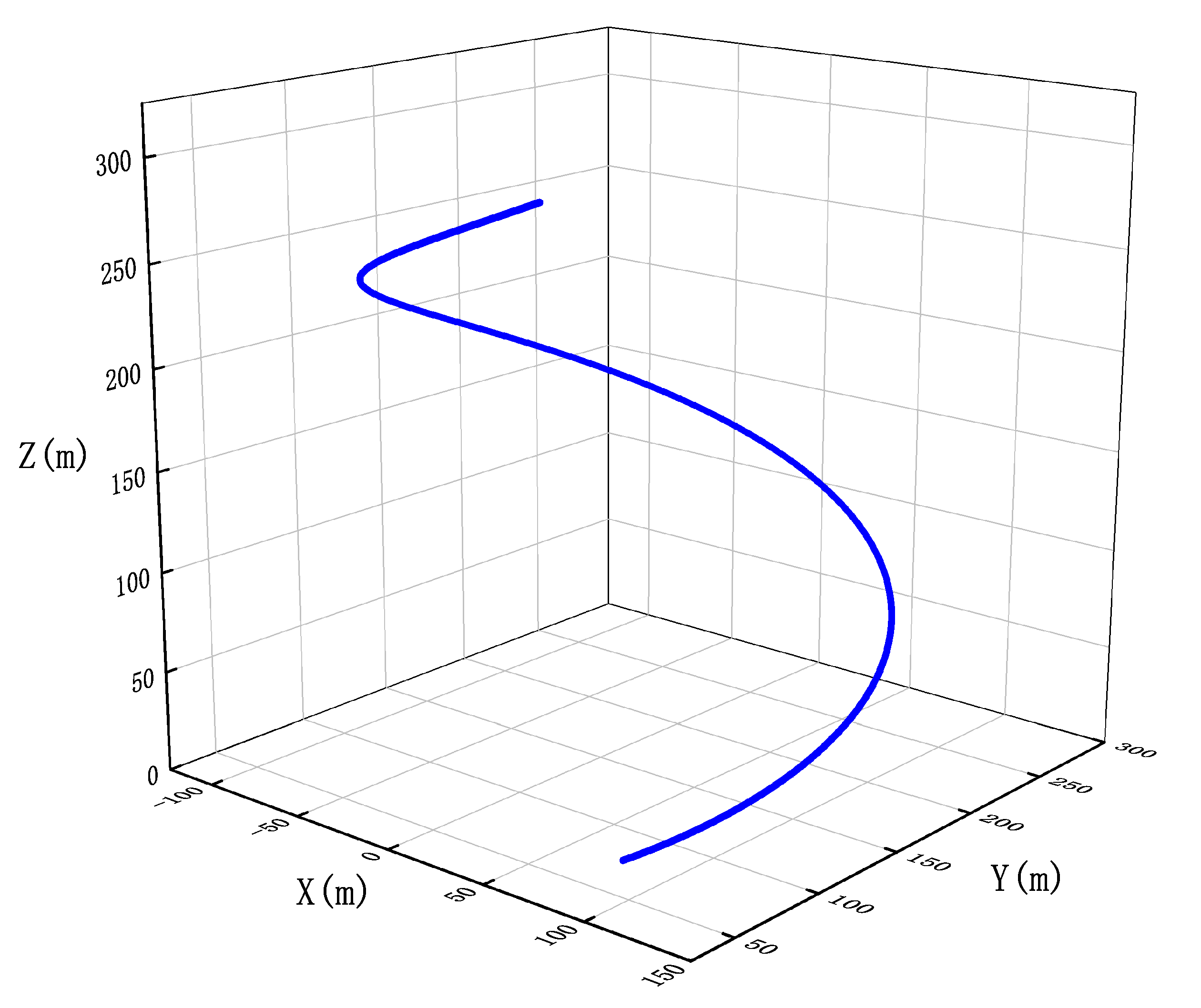
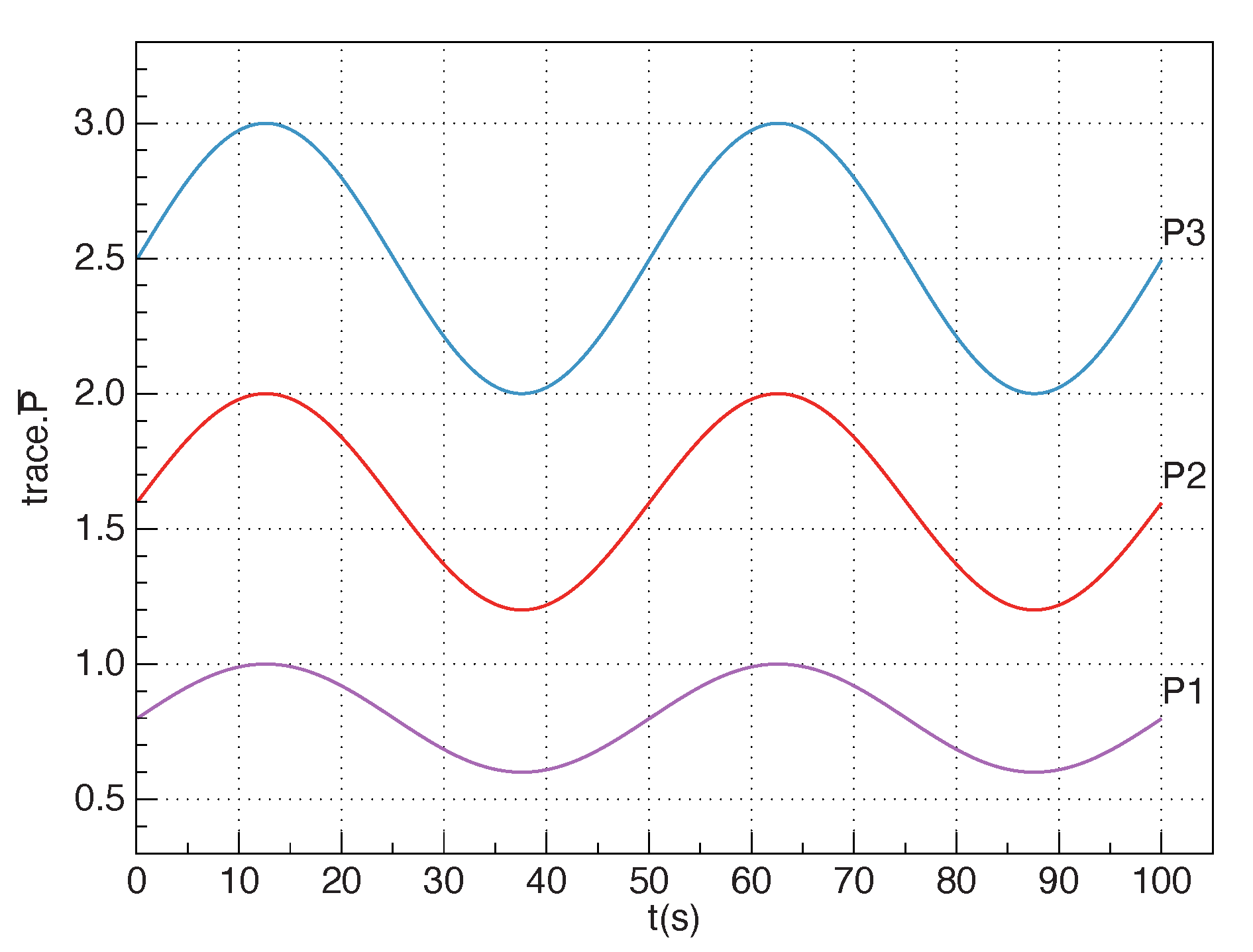
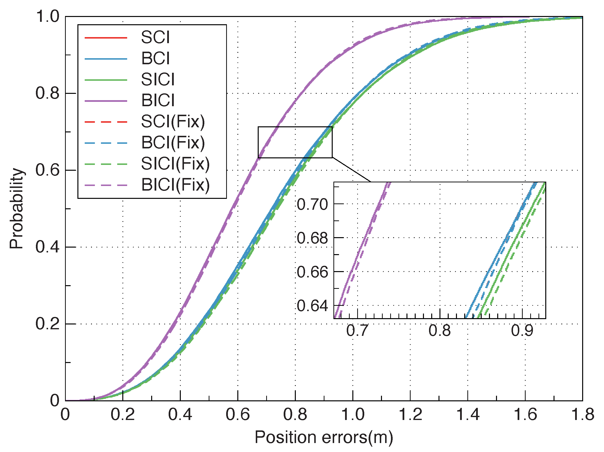
The batch forms of ICI method and the BICI multi-sensor fusion positioning algorithm are proposed based on two-sensor ICI. Meanwhile, the noise variance upper bound of error variance matrix is derived to prove the robustness of BICI. The structure of the BICI fusion algorithm is displayed in Figure 2 as follows.

Inspired by Theorem 1, the batch form of ICI is a convex combination of local filters, given as

$${\widehat{x}}_k^{BICI}=\sum _{h=1}^H{K}_h{\widehat{x}}_k^{\left(h\right)}$$

(23)

where ${\widehat{x}}_k^{\left(h\right)}$ is local filter, ${\sum }_{h=1}^H{K}_h=I$. The error variance matrix is

$${\left(P_k^{BICI}\right)}^{-1}=\sum _h{\left(P_k^h\right)}^{-1}-{\left(\sum _h{\omega }_h{P}_k^h\right)}^{-1}$$

(24)

where filtering gains $K_h$ are

$$K_h=P_k^{BICI}\left({\left(P_k^h\right)}^{-1}-{\omega }_h{\left(\sum _h{\omega }_h{P}_k^h\right)}^{-1}\right)$$

(25)

where ${\omega }_h$ fulfills the condition $0\le {\omega }_h\le 1,{\sum }_h{\omega }_h=1$. The selection of the coefficients ${\omega }_h$ is the minimum trace of the variance matrix $P_k^{BICI}$ as [15]

$$objective:\underset{\omega }{min}tr\left(P_{k|k}^{BICI\left(h\right)}\right),s.t:0\le {\omega }_h\le 1,\sum _h{\omega }_h=1.$$

(26)

The above optimization problem can also be solved by the $fmincon$ function in the MATLAB optimization toolbox.

Theorem 2.

The error variance matrix of BICI fusion algorithm is ${\tilde{P}}_k^{BICI}=E\left({\tilde{x}}_k^{BICI}{\left({\tilde{x}}_k^{BICI}\right)}^T\right)={\sum }_m{\sum }_n{K}_m{P}_k^{mn}{K}_n^T$, ${\tilde{x}}_k=x_k-{\widehat{x}}_k^{BICI}$, and noise variance upper bound is $P^{BICI}$.

Proof of Theorem 2.

$$\begin{array}{cc}\hfill E\left({\tilde{x}}_k^{BICI}{\left({\tilde{x}}_k^{BICI}\right)}^T\right)=& E\left(\left(\sum _h{K}_h{\widehat{x}}_k^{\left(h\right)}-x_k\right){\left(\sum _h{K}_h{\widehat{x}}_k^{\left(h\right)}-x_k\right)}^T\right)\hfill \\ \hfill =& E\left(\left(\sum _h{K}_h{\tilde{x}}_k^{\left(h\right)}\right){\left(\sum _h{K}_h{\tilde{x}}_k^{\left(h\right)}\right)}^T\right)\hfill \\ \hfill =& \sum _m\sum _n{K}_m{P}_k^{mn}{K}_n^T.\hfill \end{array}$$

(27)

Using the inequality is

$$K_m{P}^{mn}{K}_n^T+K_n{P}^{nm}{K}_m^T\le r{K}_m{P}^m{K}_m^T+\frac{1}{r}{K}_n{P}^n{K}_n^T$$

(28)

where $r>0$. The noise variance matrix upper bound $P_k^{BICI}$ can be subtracted by

$$\begin{array}{c}\hfill E\left({\tilde{x}}_k^{BICI}{\left({\tilde{x}}_k^{BICI}\right)}^T\right)\le \sum _h{K}_h{P}_k^h{K}_h^T+\sum _m\sum _n^m\left(r_m{K}_m{P}_k^m{K}_m^T+\frac{1}{r_m}{K}_n{P}_k^n{K}_n^T\right)=P^{BICI}.\end{array}$$

(29)

The proof is completed. □

Using Theorem 2, we demonstrated that the BICI multi-sensor fusion positioning method with unknown covariance is robust. Combined with Theorem 1, the robustness of the SICI fusion positioning method is indirectly verified as

Corollary 1.

The error variance matrix of the SICI fusion algorithm is ${\tilde{P}}_k^{SICI}=E\left({\tilde{x}}_k^{SICI}{\left({\tilde{x}}_k^{SICI}\right)}^T\right) = {\sum }_m{\sum }_n{\theta }_m^{\left(H\right)}{P}_k^{mn}{\left({\theta }_m^{\left(H\right)}\right)}^T$, ${\tilde{x}}_k=x_k-{\widehat{x}}_k^{SICI}$, and noise variance upper bound is

$P^{SICI}={\sum }_h{\theta }_h^{\left(H\right)}{P}_k^h{\left({\theta }_h^{\left(H\right)}\right)}^T+{\sum }_m{\sum }_n^m\left(r_m{\theta }_m^{\left(H\right)}{P}_k^m{\left({\theta }_m^{\left(H\right)}\right)}^T+\frac{1}{r_m}{\theta }_n^{\left(H\right)}{P}_k^n{\left({\theta }_n^{\left(H\right)}\right)}^T\right).$

3.3. Simulation

The goal of this section is to evaluate the performance of the BICI with uncertain time-varying noise variance and unknown covariance. The numerical example provides two representative cases, which are fixed and time-varying noise. The SCI, BCI, SICI and BICI multi-sensor positioning algorithms are taken for comparison. In the presentation of the simulation result, the root mean square (RMS) of positioning error is utilized for positioning accuracy and robustness evaluation.

The simulation trajectory is shown in Figure 3, and the simulation time is 100 s. A 3-sensor fusion positioning system with uncertain time-varying noise variance can be represented as

$$\begin{array}{cc}\hfill x_{k+1}=& F_k{x}_k+B_k{w}_k\hfill \end{array}$$

(30)

$$\begin{array}{cc}\hfill z_k^h=& C_k^h{x}_k+v_k^h,h=1,2,3\hfill \end{array}$$

(31)

$$B_k=\left[\begin{array}{ccc}{T}^2/2& 0& 0\\ T& 0& 0\\ 0& T^2/2& 0\\ 0& T& 0\\ 0& 0& T^2/2\\ 0& 0& T\end{array}\right]$$

(32)

$$F_k=\left[\begin{array}{cccccc}1& T& 0& 0& 0& 0\\ 0& 1& 0& 0& 0& 0\\ 0& 0& 1& T& 0& 0\\ 0& 0& 0& 1& 0& 0\\ 0& 0& 0& 0& 1& T\\ 0& 0& 0& 0& 0& 1\end{array}\right]$$

(33)

$$C_k^h=\left[\begin{array}{cccccc}1& 0& 0& 0& 0& 0\\ 0& 0& 1& 0& 0& 0\\ 0& 0& 0& 0& 1& 0\end{array}\right]$$

(34)

where $T=100$ ms is the sampling period of sensor, $x_k={\left[p_x,v_x,p_y,v_y,p_z,v_z\right]}^T$ is the positioning system state. $p_x$, $p_y$ and $p_z$ are the position of X, Y and Z directions, respectively. $v_x$, $v_y$ and $v_z$ are the velocity of X, Y and Z directions, respectively. $w_k$ and $v_k^h$ are white Gaussian noise with zero mean and variance matrix ${\overline{Q}}_k$, ${\overline{R}}_k^h$, respectively. In the simulation, we take $Q=3I$, ${\overline{Q}}_k=0.8$ and the conservative accuracy of three sensors as 1 m, 2 m and 3 m, respectively. The observation and process noise of sensors 1 and 2 have random correlation coefficients of ${\rho }_k^{{\omega }_k}$ and ${\rho }_k^{v_k^{(1,2)}}$, respectively. ${\rho }_k^{{\omega }_k}\in [0.1,0.3]$, ${\rho }_k^{v_k^{(1,2)}}\in [0.1,0.2]$.

The true trace of the fixed noise variance matrix of about three sensors is $0.8$ m, $1.6$ m and $2.5$ m, respectively. The trace of the time-varying noise variance matrix is $0.8+0.2sin(2\pi kT/50)$ m, $1.6+0.4sin(2\pi kT/50)$ m and $2.5/3+0.5/3sin(2\pi kT/50)$ m. The time-varying trace of three sensors is shown in Figure 4.

Through 50 Monte Carlo simulations, the cumulative distribution functions (CDF) of SCI, BCI, SICI, BICI, SCI (fix), BCI (fix), SICI (fix) and BICI (fix) with uncertain time-varying noise are shown in Figure 5. It is indicated that SCI, BCI, SICI, and BICI multi-sensor fusion positioning algorithms have the same positioning accuracy under uncertain fixed and time-varying noise variance, respectively. Therefore, the four algorithms have good robustness under the time-varying noise variance. The positioning accuracy relation is $SICI<BCI\approx SCI<BICI$ in

Table 1. RMS of positioning error.

Algorithms	Positioning Error (m)
SCI	0.88
BCI	0.88
SICI	0.90
BICI	0.71
SCI (fix)	0.88
BCI (fix)	0.88
SICI (fix)	0.90
BICI (fix)	0.71

. BICI has less conservativeness and improved the positioning accuracy by at least 26.7% compared with the other three algorithms.

4. Multi-Sensor Fusion Positioning Algorithm Based on BICI and IMM

The motion pattern of platform is typically hard to obtain in actual scene. The filter based on a single model sharpens the deterioration of positioning accuracy and divergences when motion model noise variance exceeds the conservative upper bound in the strong mobility scenario. The accurate estimation can be obtained by a multi-model algorithm with known covariance in actual scene. There are few studies on the estimation with uncertain time-varying noise variance. Combined with BICI and IMM, BICI-IMM multi-sensor fusion positioning algorithm improves the positioning accuracy.

The process of the traditional IMM algorithm is divided into four steps: model reinitialization, model filter, model probability updating and estimation fusion [34]. The model filter designs for a single sensor cannot meet the multi-sensor fusion positioning. Therefore, we introduced a local model and global filter to replace model filter based on BICI algorithm. Meanwhile, a sequential method was employed for the likelihood function in the model probability updating phase.

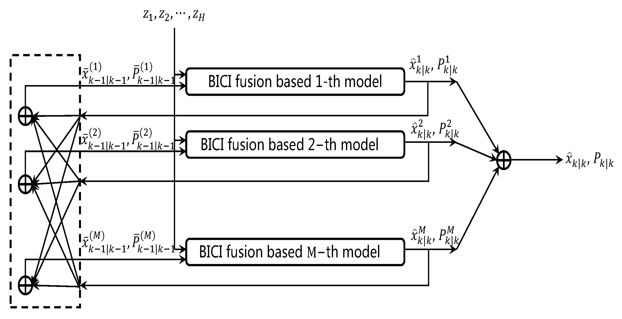
4.1. BICI-IMM Algorithm

The structure of the BICI-IMM fusion algorithm is shown in Figure 6.

Consider a multi-sensor fusion positioning system with an unknown motion model and uncertain time-varying noise variance as

$$\begin{array}{cc}\hfill x_{k+1}^i=& F_k^i{x}_k^i+B_k^i{w}_k^i,i=1,2,\cdots ,M\hfill \end{array}$$

(35)

$$\begin{array}{cc}\hfill z_k^h=& C_k^h{x}_k+v_k^h,h=1,2,\cdots ,H\hfill \end{array}$$

(36)

where M represents the number of models, H represents the number of sensors. During one filtering update cycle, the BICI-IMM algorithm assumes that the motion model is transferred from model i to j with an a priori transfer probability ${\pi }_{ij}$ defined as

$${\pi }_{ij}=P\left\{m_k^j\right|m_k^i,s_k\in \mathbb{M}\}$$

(37)

where $\mathbb{M}=\{m_k^i,i=1,2,\dots ,M\}$ is the model set, ${\sum }_j{\pi }_{ij}=1$. It is assumed that the local estimation of h-th sensor of j-th model at time $k-1$ is ${\widehat{x}}_{k-1|k-1}^{j,h}$, the corresponding estimation error variance matrix is $P_{k-1|k-1}^{j,h}$. The global estimation of j-th model is ${\widehat{x}}_{k-1|k-1}^j$ and error variance matrix is $P_{k-1|k-1}^j$. The model probability is $u_{k-1}^j$. The process of BICI-IMM algorithm at time k is

(1) Model reinitialization

For $i=1,2,\dots ,M$, the model prediction probability is defined as

$$u_{k|k-1}^i=P\left\{m_k^i|z^{k-1}\right\}=\sum _j{\pi }_{ji}{u}_{k-1}^j.$$

(38)

The interaction weight is defined as

$$u_{k-1}^{j|i}=P\left\{m_{k-1}^j|m_k^i,z^{k-1}\right\}={\pi }_{ji}{u}_{k-1}^j/u_{k|k-1}^i.$$

(39)

The interaction state estimation and variance matrix are

$${\overline{x}}_{k-1|k-1}^{i,h}=E\left\{x_{k-1}|m_k^i,{\mathcal{M}}_{k-1},z^{k-1}\right\}=\sum _j{u}_{k-1}^{j|i}{\widehat{x}}_{k-1|k-1}^j,h=1,2,\dots ,H$$

(40)

$${\overline{P}}_{k-1|k-1}^{i,h}=\sum _j\left[P_{k-1|k-1}^{j,h}+\left({\overline{x}}_{k-1|k-1}^{i,h}-{\widehat{x}}_{k-1|k-1}^j\right){\left({\overline{x}}_{k-1|k-1}^{i,h}-{\widehat{x}}_{k-1|k-1}^j\right)}^T\right]u_{k-1}^{j|i}.$$

(41)

(2) Model local filter

For h-th sensor ($h=1,2,\dots ,H$), the local state estimation process is

$$u_{k|k-1}^i=P\left\{m_k^i|z^{k-1}\right\}=\sum _j{\pi }_{ji}{u}_{k-1}^j.$$

(42)

The state prediction is

$${\widehat{x}}_{k|k-1}^{i,h}=F_k^{i,h}{\widehat{X}}_{k-1|k-1}^i,h=1,2,\dots ,H$$

(43)

where the variance of positioning prediction error is

$$P_{k|k-1}^{i,h}=F_k^{i,h}{{\overline{P}}_{k-1|k-1}^{i,h}{F}_k^{i,h}}^T+B_k^i{Q_{ka}{B}_k^i}^T.$$

(44)

The measurement residual is

$${\tilde{z}}_k^{i,h}=z_k^h-C_k^h{\widehat{x}}_{k|k-1}^{i,h}.$$

(45)

The measurement noise variance matrix is

$${S^{i,h}=C}_k^h{P}_{k|k-1}^h{C_k^h}^T+R_k^h.$$

(46)

The filtering gain is

$$G_k^{i,h}=C_k^h{P}_{k|k-1}^{i,h}{{(S}^{i,h})}^{-1}.$$

(47)

Update the state estimation and variance matrix to

$${\widehat{x}}_{k|k}^{i,h}={\widehat{x}}_{k|k-1}^{i,h}+G_k^{i,h}{\tilde{z}}_k^{i,h}$$

(48)

$$P_{k|k}^{i,h}=(I-G_k^{i,h}{C}_k^h)P_{k|k-1}^{i,h}.$$

(49)

(3) Global filter

The global estimation of j-th model based on the BICI algorithm is

$${\widehat{x}}_k^j=\sum _{h=1}^H{K_h^j\widehat{x}}_{k+1}^{j,h}$$

(50)

with error variance matrix is

$${{(P}_k^j)}^{-1}={\sum _h\left(P_k^{j,h}\right)}^{-1}-{\left(\sum _h{\omega }_h^j{P}_k^{j,h}\right)}^{-1}$$

(51)

where $K_h^j$, ${\omega }_h^j$ are determined by Equations (14) and (26), respectively.

(4) Calculation model likelihood probability function

For i-th model ($i=1,2,\dots ,M$), h-th sensor ($h=1,2,\dots ,H$), the updated probability of model $m_k^i$ probability is

$${\Lambda }_k^{i,h}=p\left({\tilde{z}}_k^{i,h}|m_k^i,z_{k-1}^{i,h}\right).$$

(52)

The likelihood function is obtained through multi-dimensional normal distribution distribution by

$${\Lambda }_k^{i,h}=p\left({\tilde{z}}_k^{i,h}|m_k^i,z_{k-1}^{i,h}\right)={\left|{\left(2\pi \right)}^H{S}^{i,h}\right|}^{-\frac{1}{2}}{e}^{\left\{-\frac{1}{2}{\left({\tilde{z}}_k^{i,h}\right)}^T{\left(S_k^{i,h}\right)}^{-1}{\tilde{z}}_k^{i,h}\right\}}.$$

(53)

The recursive formula of updating the model probability at time k through the model likelihood function based on the sequential method is

$$U_k^{i,h}=\frac{U_{k|k-1}^{i,h-1}{\Lambda }_k^{i,h}}{{\sum }_j{U}_{k|k-1}^{j,h-1}{\Lambda }_k^{j,h}}$$

(54)

$$U_{k|k-1}^{i,h}=\sum _j{\pi }_{ji}{U}_k^{j,h},h=1,2,\dots ,H-1$$

(55)

where the initial value is

$$U_{k|k-1}^{i,0}=u_k^{i,1},i=1,2,\dots ,M.$$

(56)

The probability of the updated model is

$$u_k^i=U^{i,H-1}.$$

(57)

(5) Estimation fusion

The weighted sum of state estimation of model filters is taken as the global estimation, so the global estimation and noise variance matrix are

$${\widehat{x}}_{k|k}=\sum _i{\widehat{x}}_{k|k}^i{u}_k^i$$

(58)

$$P_{k|k}=\sum _i{u}_k^i\left[P_{k|k}^i+\left({\widehat{x}}_k-{\widehat{x}}_{k|k}^i\right){\left({\widehat{x}}_k-{\widehat{x}}_{k|k}^i\right)}^T\right].$$

(59)

4.2. Simulation

In order to evaluate the positioning accuracy of the BICI-IMM multi-sensor fusion positioning algorithm with uncertain noise variance, unknown covariance and motion model, we simulated the unmanned platform with constant velocity (CV) and constant turn (CT) models. The positioning accuracy evaluation is the same as in Section 3.3. The multi-sensor positioning system model is shown as

$$x_{k+1}^i=F_k^i{x}_k^i+B_k^i{w}_k^i,i=1,2$$

(60)

$$z_k^h=C_k^h{x}_k+v_k^h,h=1,2,3.$$

(61)

(1) The CV model

It is assumed that the unmanned platform moves in a straight line with constant speed and the system state is $x_k={\left[p_x,v_x,p_y,v_y\right]}^T$; then

$$F_{CV}=\left[\begin{array}{cccc}1& T& 0& 0\\ 0& 1& 0& 0\\ 0& 0& 1& T\\ 0& 0& 0& 1\end{array}\right]$$

(62)

$$B_{CV}=\left[\begin{array}{cc}{T}^2/2& 0\\ T& 0\\ 0& T^2/2\\ 0& T\end{array}\right].$$

(63)

(2) The CT model

It is assumed that unmanned platform moves in a turning motion at constant angular speed $\psi$ and the system state is $x_k={\left[p_x,v_x,p_y,v_y\right]}^T$, then

$$F_{CT}=\left[\begin{array}{cccc}1& \frac{sin\psi T}{\psi }& 0& -\frac{1-cos\psi T}{\psi }\\ 0& cos\psi T& 0& -sin\psi T\\ 0& \frac{1-cos\psi T}{\psi }& 1& \frac{sin\psi T}{\psi }\\ 0& sin\psi T& 0& cos\psi T\end{array}\right]$$

(64)

$$B_{CT}=\left[\begin{array}{cc}{T}^2/2& 0\\ T& 0\\ 0& T^2/2\\ 0& T\end{array}\right].$$

(65)

The trajectory of the unmanned platform is displayed in Figure 7, which contains CV and CT models in

Table 2. Motion model settings.

Time (s)	Motion Model
$[0,50)$	CV
$[50,70)$	CT
$[70,120)$	CV
$[120,140)$	CT
$[140,190)$	CV
$[190,210)$	CT

. The initial state is $X_0={[10,5,10,0]}^T$. In the simulation, we take $Q=3I$, ${\overline{Q}}_k=0.8$, and the conservative noise variance upper bounds of the three sensors are 1 m, 2 m and 3 m, respectively. The actual positioning accuracies of the three sensors are $0.8$ m, $1.2$ m and 2 m, respectively. The correlation coefficients of sensor 1 and 2 are the same as in Section 3.3.

Through 50 Monte Carlo simulations, the positioning results of BICI, SICI and BICI-IMM are exhibited in Figure 8. Figure 9 is the positioning error CDF of algorithms. It is indicated that BICI has a higher positioning accuracy compared with other single model algorithms. In contrast, the BICI-IMM has higher positioning accuracy. The algorithm based on CV model positioning accuracy is slightly higher than the model based on CT in

Table 3. RMS position error (m).

Algorithm	RMS Positioning Error (m)
BICI-IMM	0.47
BICI (CV)	0.53
BICI (CT)	0.56
SICI (CV)	0.70
SICI (CT)	0.71

.

The error variance of system model based on CV is relatively, small because 71% and 29% of the motion model are CV and CT. Therefore, the positioning accuracy is also slightly higher. The positioning accuracy of BICI-IMM algorithm is about 14.3% and 52%, increased by the BICI and SICI algorithm, respectively.

5. Experiment

In order to verify the positioning accuracy of the BICI-IMM and BICI fusion positioning algorithms, we designed a multi-sensor fusion positioning equipment and carried out the fusion positioning algorithms experiments in the open and semi-open areas. As shown in Figure 10, the multi-sensor fusion positioning equipment includes two GPS, IMU, co-processor and embedded CPU. The two GPS receivers adopt ZED-F9P and MAX-7Q of u-blox company. The IMU sensor is the ADIS16470. The co-processor adopts the STM32F407 with uC/OS-III for data acquisition and time synchronization between sensors. The collected sensors data are sent to the embedded processor through rosserial. The embedded CPU is Allwinner H6 and carries a Linux operating system with a robot operating system. Allwinner H6 is the sensors’ data-processing unit for data recording and fusion processing. During the experiment, we used the high-precision real-time kinematic (RTK) receiver of CHCNV E91 as the reference positioning and the continuously operating reference stations (CORS) adopted the FindCM service of Qianxun.

5.1. Open Area Experiment

We carried out the positioning accuracy of multi-sensor fusion positioning experiment based on fusion positioning equipment in the playground, as in Figure 11 of Beijing University of Posts and Telecommunications. We walked around the playground with positioning equipment and CHCNV E91. The fusion positioning results of SICI(CV), SICI(CT), BICI(CV), BICI(CT) and BICI-IMM algorithms are presented in Figure 12. The RMS positioning errors of SICI(CV), SICI(CT), BICI(CV), BICI(CT) and BICI-IMM fusion positioning algorithms are 1.559 m, 1.561 m, 1.49 m, 1.484 m and 1.27 m as shown in

Table 4. RMS position error in open area.

Algorithms	Positioning Error (m)
BICI-IMM	1.27
BICI (CV)	1.49
BICI (CT)	1.484
SICI (CV)	1.559
SICI (CT)	1.561

and Figure 13. Compared with single model BICI and SICI algorithms, the positioning accuracies of the BICI-IMM multi-sensor fusion algorithm are improved by 18.5% and 14.4%, respectively. Therefore, the BICI-IMM multi-sensor fusion algorithm has better positioning accuracy in open area.

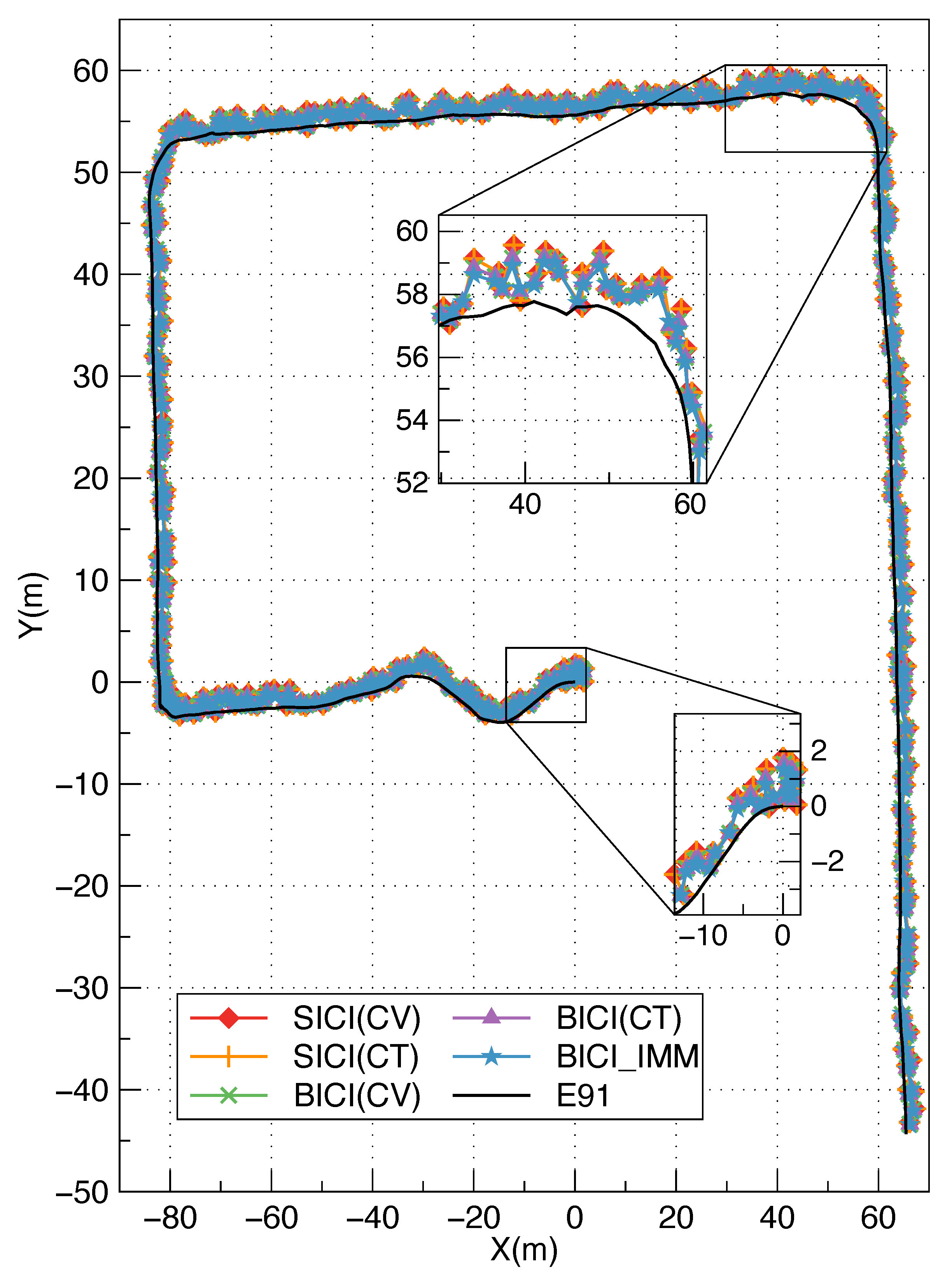
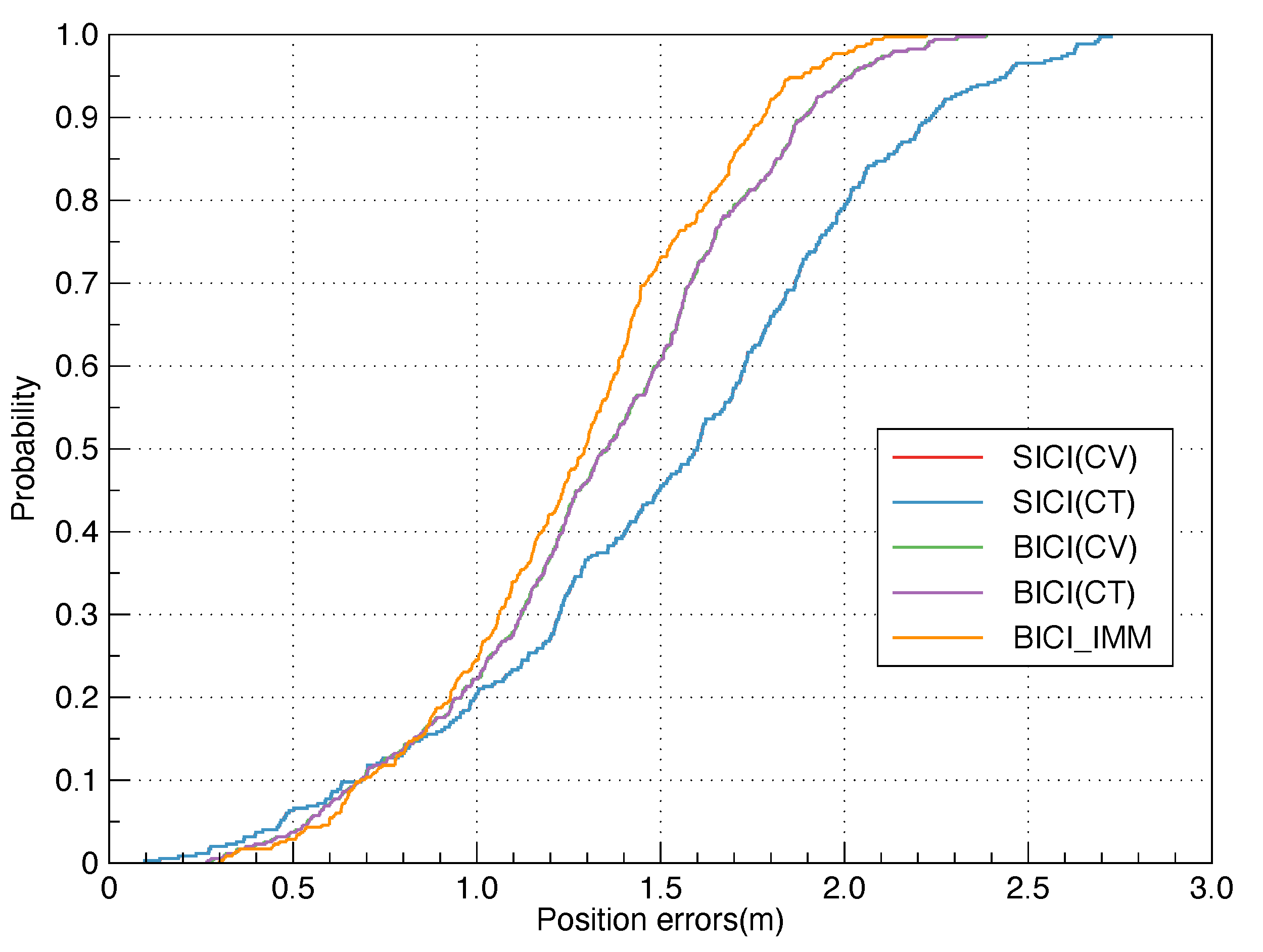
5.2. Semi-Open Area Experiment

We demonstrated the fusion positioning accuracy of the experiment under the semi-open area as in Figure 14, in front of the 4th teaching building of Beijing University of Posts and Telecommunications. The positioning results of SICI(CV), SICI(CT), BICI(CV), BICI(CT) and BICI-IMM algorithms are shown in Figure 15. The positioning errors are statistically analyzed in Figure 16. The RMS positioning errors of SICI(CV), SICI(CT), BICI(CV), BICI(CT) and BICI-IMM fusion positioning algorithms are 1.838 m, 1.839 m, 1.564 m, 1.563 m and 1.44 m in

Table 5. RMS position error in the semi-open area.

Algorithms	Positioning Error (m)
BICI-IMM	1.44
BICI (CV)	1.564
BICI (CT)	1.563
SICI (CV)	1.838
SICI (CT)	1.839

. Compared with other algorithms, the accuracy of the BICI fusion positioning algorithm decreases the least, so BICI has better robustness and positioning accuracy. However, the performance of BICI-IMM is limited by the precision motion model, which is hard to obtain.

6. Discussion

With respect the local filter, the sensor subsystem is a linear system. For the nonlinear system, the extending Kalman is one of the solutions. The robustness and other research need to be further improved for complex scenarios.

The $H-$1 dimension optimization is inevitable for BICI. The fast calculation method of the CI method can be used as a reference [35], which reduces the computational complexity of the BICI algorithm and fits the real-time positioning and navigation for the embedded platform with computing and power consumption limitation.

In multi-model algorithm, BICI-IMM utilizes a fixed model set. The size of the model set will be very large in the actual scene. It will boost the computational complexity and positioning error due to the conflicts among the motion models. The variable-structure multi-model algorithm can achieve a balanced positioning accuracy, model set size and computational complexity. Therefore, it is necessary for the further study of a fusion positioning algorithm based on a variable-structure multiple-model, in order to enhance positioning accuracy in challenging scenes.

7. Conclusions

A BICI multi-sensor fusion positioning algorithm is proposed based on the batch form of ICI. Compared with SICI, BCI and SCI algorithm, the positioning accuracy of the BICI algorithm increases by 26.7%, at least in the simulation. We presented the BICI-IMM algorithm with unknown motion model, uncertain time-varying noise variance and unknown covariance based on an IMM algorithm structure. The positioning accuracy increased by 14.3% compared with BICI. The BICI-IMM multi-sensor fusion algorithm has better positioning accuracy than SICI in the open and semi-open scenes. The BICI-IMM can provide a robust positioning for the distributed control of robots and assist in the rapid construction of dynamical network topologies [36]. It helps to decrease the average time taken to organize the group in a coordinated behavior and increase the moving speed of robots in real applications.

References

1. Cheng, L.; Huang, S.; Xue, M.; Bi, Y. A Robust Localization Algorithm Based on NLOS Identification and Classification Filtering for Wireless Sensor Network. Sensors 2020, 20, 6634. [Google Scholar] [CrossRef]
2. Kułakowski, P.; Vales-Alonso, J.; Egea-López, E.; Ludwin, W.; García-Haro, J. Angle-of-arrival localization based on antenna arrays for wireless sensor networks. Comput. Electr. Eng. 2010, 36, 1181–1186. [Google Scholar] [CrossRef]
3. Xue, W.; Qiu, W.; Hua, X.; Yu, K. Improved Wi-Fi RSSI measurement for indoor localization. IEEE Sens. J. 2017, 17, 2224–2230. [Google Scholar] [CrossRef]
4. Wu, P.; Su, S.; Zuo, Z.; Guo, X.; Sun, B.; Wen, X. Time difference of arrival (TDoA) localization combining weighted least squares and firefly algorithm. Sensors 2019, 19, 2554. [Google Scholar] [CrossRef] [Green Version]
5. Yu, X.M.; Wang, H.Q.; Wu, J.Q. A method of fingerprint indoor localization based on received signal strength difference by using compressive sensing. Eurasip. J. Wirel. Commun. Netw. 2020, 2020, 72. [Google Scholar] [CrossRef]
6. Shirehjini, A.A.N.; Yassine, A.; Shirmohammadi, S. An RFID-Based Position and Orientation Measurement System for Mobile Objects in Intelligent Environments. IEEE Trans. Instrum. Meas. 2012, 61, 1664–1675. [Google Scholar] [CrossRef]
7. Zhou, S.; Pollard, J.K. Position measurement using Bluetooth. IEEE Trans. Consum. Electr. 2006, 52, 555–558. [Google Scholar] [CrossRef]
8. Qin, T.; Li, P.; Shen, S. VINS-Mono: A Robust and Versatile Monocular Visual-Inertial State Estimator. IEEE Trans. Robot 2018, 34, 1004–1020. [Google Scholar] [CrossRef] [Green Version]
9. Xu, H.; Wang, L.; Zhang, Y.; Qiu, K.; Shen, S. Decentralized Visual-Inertial-UWB Fusion for Relative State Estimation of Aerial Swarm. In Proceedings of the 2020 IEEE International Conference on Robotics and Automation (ICRA), Paris, France, 31 May–31 August 2020; pp. 8776–8782. [Google Scholar] [CrossRef]
10. Han, Y. Optical Flow/INS Navigation System in Four-rotor. In Proceedings of the 2019 5th International Conference on Systems, Control and Communications, Wuhan, China, 21–23 December 2019; pp. 1–5. [Google Scholar]
11. Fung, M.L.; Chen, M.Z.; Chen, Y.H. Sensor fusion: A review of methods and applications. In Proceedings of the 2017 29th Chinese Control And Decision Conference (CCDC), Chongqing, China, 28–30 May 2017; pp. 3853–3860. [Google Scholar]
12. Hubert, M.; Debruyne, M.; Rousseeuw, P.J. Minimum covariance determinant and extensions. Wiley Interdiscip. Rev. Comput. Stat. 2018, 10, e1421. [Google Scholar] [CrossRef] [Green Version]
13. Kalina, J. The minimum weighted covariance determinant estimator revisited. Commun. Stat. Simul. Comput. 2020, 1–13. [Google Scholar] [CrossRef]
14. Julier, S.J.; Uhlmann, J.K. A non-divergent estimation algorithm in the presence of unknown correlations. Proc. Am. Control Conf. 1997, 4, 2369–2373. [Google Scholar]
15. Munz, M.; Mahlisch, M.; Dietmayer, K. Generic Centralized Multi Sensor Data Fusion Based on Probabilistic Sensor and Environment Models for Driver Assistance Systems. IEEE Intell. Transp. Syst. Mag. 2010, 2, 6–17. [Google Scholar] [CrossRef]
16. Deng, Z.; Zhang, P.; Qi, W.; Liu, J.; Gao, Y. Sequential covariance intersection fusion Kalman filter. Inf. Sci. Int. J. 2012, 189, 293–309. [Google Scholar] [CrossRef]
17. Zhang, P.; Qi, W.J.; Deng, Z.L. Parallel Covariance Intersection Fusion Optimal Kalman Filter. Appl. Mech. Mater. 2013, 475, 436–441. [Google Scholar] [CrossRef]
18. Sijs, J.; Lazar, M. State fusion with unknown correlation: Ellipsoidal intersection. Automatica 2012, 48, 1874–1878. [Google Scholar] [CrossRef] [Green Version]
19. Zarei-Jalalabadi, M.; Malaek, S.M.B.; Kia, S.S. A Track-to-Track Fusion Method for Tracks With Unknown Correlations. IEEE Control Syst. Lett. 2017, 2, 189–194. [Google Scholar] [CrossRef]
20. Noack, B.; Sijs, J.; Hanebeck, U.D. Algebraic analysis of data fusion with ellipsoidal intersection. In Proceedings of the IEEE International Conference on Multisensor Fusion & Integration for Intelligent Systems, Baden-Baden, Germany, 19–21 September 2017. [Google Scholar]
21. Noack, B.; Sijs, J.; Reinhardt, M.; Hanebeck, U.D. Decentralized data fusion with inverse covariance intersection. Automatica 2017, 79, 35–41. [Google Scholar] [CrossRef]
22. Chen, L.; Yu, K.; Wu, K.; Gao, Y.; Huo, Y.; Ran, C.; Dou, Y. Sequential Inverse Covariance Intersection Fusion Kalman Filter for Multi-sensor Systems with Packet Dropouts and Multiplicative Noise. In Proceedings of the 2020 Chinese Automation Congress (CAC), Shanghai, China, 6–8 November 2020; pp. 1335–1340. [Google Scholar]
23. Tang, M.; Rong, Y.; Zhou, J.; Li, X.R. Information geometric approach to multisensor estimation fusion. IEEE Trans. Signal Process. 2018, 67, 279–292. [Google Scholar] [CrossRef]
24. Blom, H.A. An efficient filter for abruptly changing systems. In Proceedings of the 23rd IEEE Conference on Decision and Control, Las Vegas, NV, USA, 12–14 December 1984; pp. 656–658. [Google Scholar]
25. Visina, R.; Bar-Shalom, Y.; Willett, P.; Dey, D. On-demand track-to-track fusion using local IMM inside information. In Proceedings of the Signal Processing, Sensor/Information Fusion, and Target Recognition XXVIII, Baltimore, MD, USA, 15–17 April 2019; International Society for Optics and Photonics: Bellingham, WA, USA, 2019; Volume 11018, p. 1101804. [Google Scholar]
26. Li, W.; Jia, Y. An information theoretic approach to interacting multiple model estimation. IEEE Trans. Aerosp. Electron. Syst. 2015, 51, 1811–1825. [Google Scholar] [CrossRef]
27. Li, L.; Wu, S.; Li, X. Multi-Object Tracking Based on Deep Probability Fusion with Holistic Feature Reprentation and IMM-JIPDA. In Proceedings of the 2019 16th International Computer Conference on Wavelet Active Media Technology and Information Processing, Chengdu, China, 14–15 December 2019; pp. 295–302. [Google Scholar]
28. Ma, Y.; Zhao, S.; Huang, B. Multiple-model state estimation based on variational Bayesian inference. IEEE Trans. Autom. Contrl 2018, 64, 1679–1685. [Google Scholar] [CrossRef]
29. Wang, N.; Li, Y.; Cong, J.; Sheng, A. Sequential covariance intersection-based Kalman consensus filter with intermittent observations. IET Signal Process 2020, 14, 624–633. [Google Scholar] [CrossRef]
30. Huber, P.J. Robust Statistics; John Wiley & Sons: Hoboken, NJ, USA, 2004; Volume 523. [Google Scholar]
31. Qi, W.J.; Zhang, P.; Nie, G.H.; Deng, Z.L. Robust weighted fusion Kalman predictors with uncertain noise variances. Digit. Signal Process. 2014, 30, 37–54. [Google Scholar] [CrossRef]
32. Kailath, T.; Sayed, A.H.; Hassibi, B. Linear Estimation; Number Book; Prentice Hall: Hoboken, NJ, USA, 2000. [Google Scholar]
33. Zhu, C.; Xia, Y.; Xie, L.; Yan, L. Optimal linear estimation for systems with transmission delays and packet dropouts. IET Signal Process 2013, 7, 814–823. [Google Scholar] [CrossRef]
34. Kirubarajan, T.; Bar-Shalom, Y.; Pattipati, K.R.; Kadar, I. Ground target tracking with variable structure IMM estimator. IEEE Trans. Aerosp. Electron. Syst. 2000, 36, 26–46. [Google Scholar] [CrossRef]
35. Niehsen, W. Information fusion based on fast covariance intersection filtering. In Proceedings of the Fifth International Conference on Information Fusion, FUSION 2002 (IEEE Cat. No. 02EX5997), Annapolis, MD, USA, 8–11 July 2002; Volume 2, pp. 901–904. [Google Scholar]
36. Buscarino, A.; Fortuna, L.; Frasca, M.; Rizzo, A. Dynamical network interactions in distributed control of robots. Chaos Interdiscip. J. Nonlinear Sci. 2006, 16, 015116. [Google Scholar] [CrossRef]
Figure 1. SICI multi-sensor fusion algorithm structure.
Applsci 11 04908 g001
Figure 2. BICI multi-sensor fusion algorithm structure.
Applsci 11 04908 g002
Figure 3. The simulation trajectory of three-dimensional motion.
Applsci 11 04908 g003
Figure 4. The true trace of time-varying noise variance matrix.
Applsci 11 04908 g004
Figure 5. The positioning error CDF of three-dimensional motion.
Applsci 11 04908 g005
Figure 6. BICI-IMM multi-sensor fusion algorithm structure.
Applsci 11 04908 g006
Figure 7. The simulation trajectory of two-dimensional motion.
Applsci 11 04908 g007
Figure 8. Comparison of positioning results.
Applsci 11 04908 g008
Figure 9. The positioning error CDF of two-dimensional motion.
Applsci 11 04908 g009
Figure 10. The hardware of multi-sensor fusion positioning equipment.
Applsci 11 04908 g010
Figure 11. Open area scene.
Applsci 11 04908 g011
Figure 12. Comparison of positioning results in the open area (local Cartesian coordinates coordinate system).
Applsci 11 04908 g012
Figure 13. The CDF of positioning error in open area.
Applsci 11 04908 g013
Figure 14. Semi-open area scene.
Applsci 11 04908 g014
Figure 15. Comparison of positioning results in the semi-open area (local Cartesian coordinates coordinate system).
Applsci 11 04908 g015
Figure 16. The CDF of positioning error in the semi-open area.
Applsci 11 04908 g016