
Building Survivable Software Systems by Automatically Adapting to Sensor Changes


Abstract
1. Introduction
2. Settings and Notations
2.1. Settings
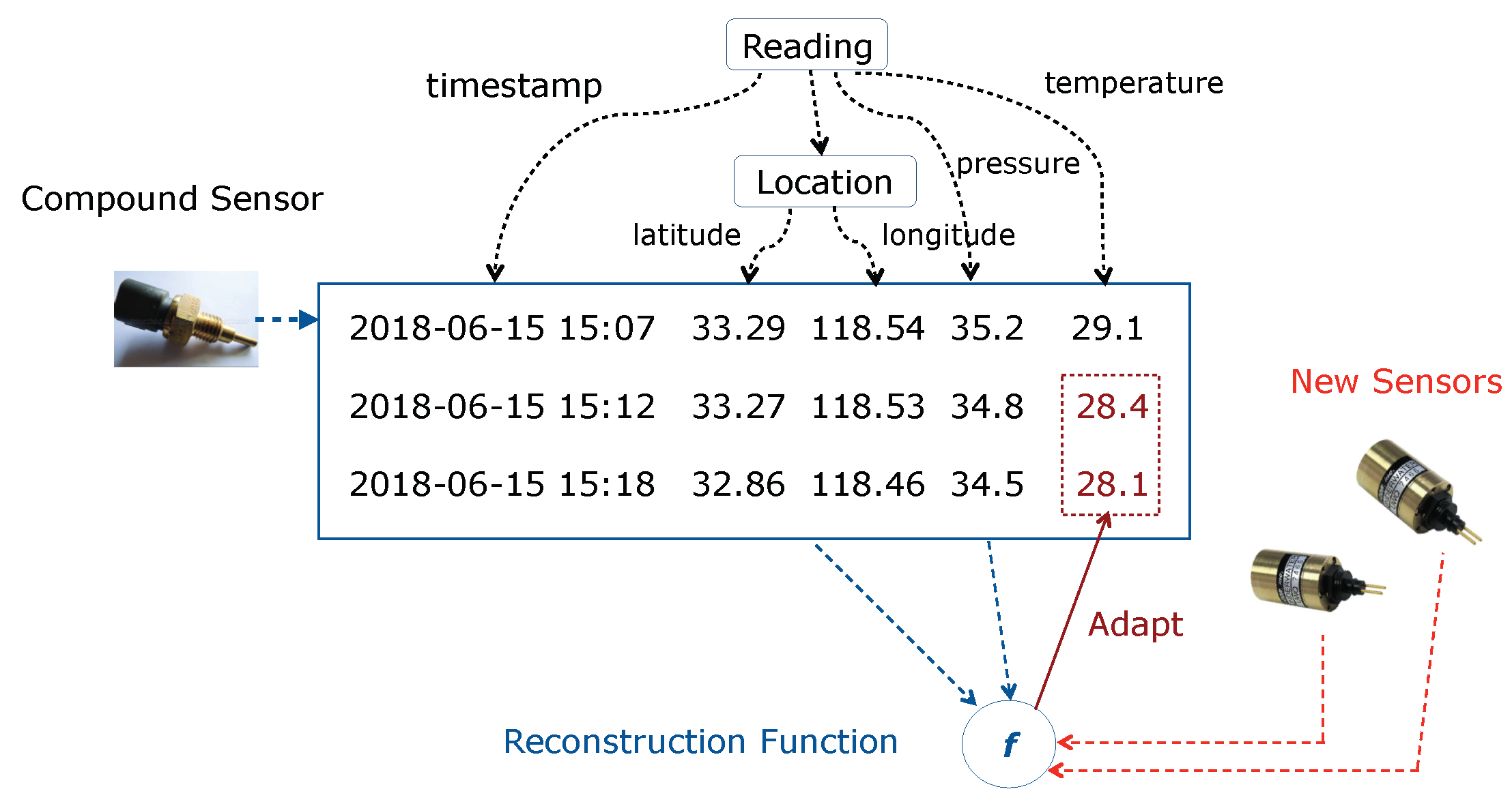
- Individual Sensor Change: some but not all of the individual sensors in a compound sensor are replaced by another set of individual sensors. This corresponds to the cases where new individual sensors are plugged in manually or automatically when sensor failures or sensor upgrades occur.
- Compound Sensor Change: the entire compound sensor is replaced by a new compound sensor. This happens in practice for the reason that replacing the compound sensor is technically easier than replacing individual sensors in certain systems. This scenario is more challenging than individual sensor change, since no individual sensor from the compound sensor can be used to calibrate the new sensors.
- Reference sensors always work properly.
- Replaced sensors are replaced by new sensors at the change point.
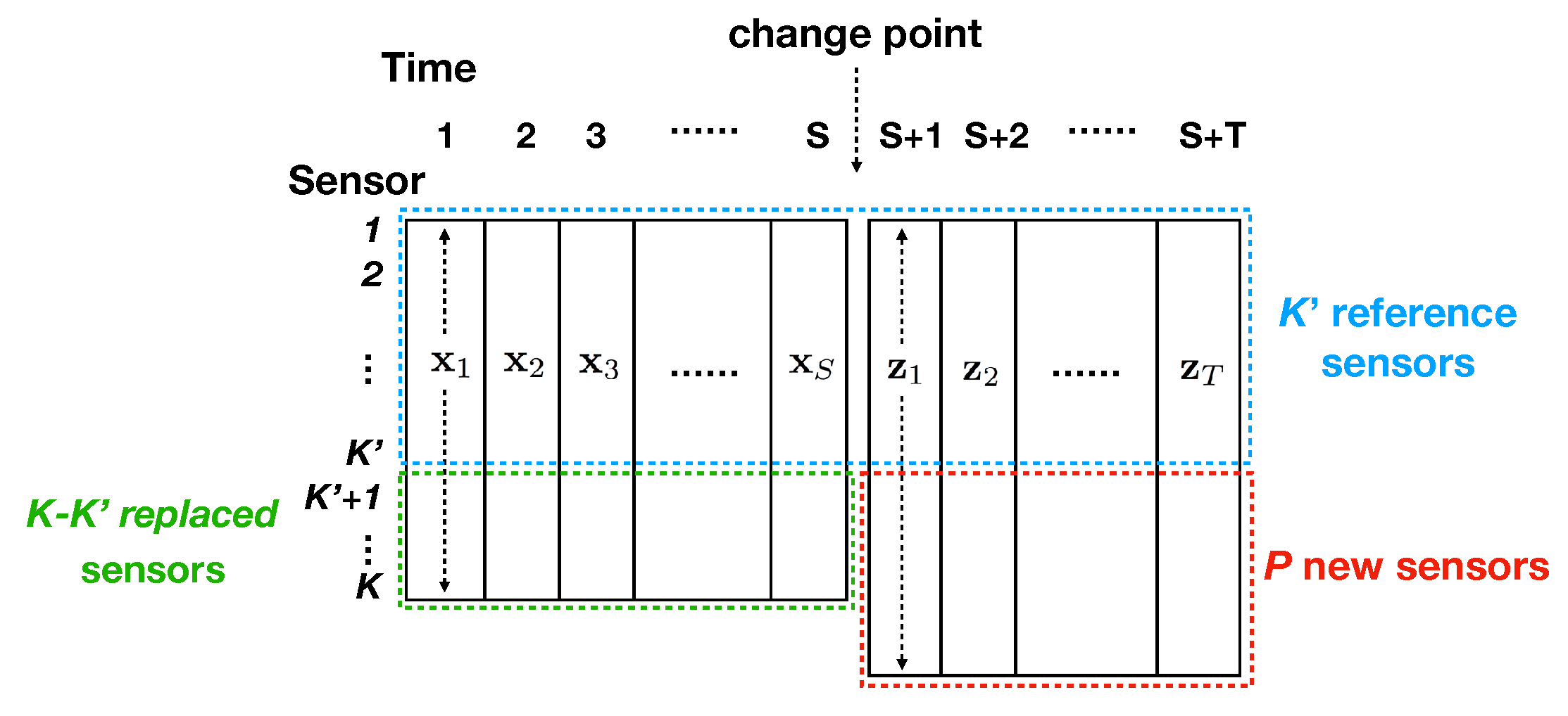
2.2. Notations
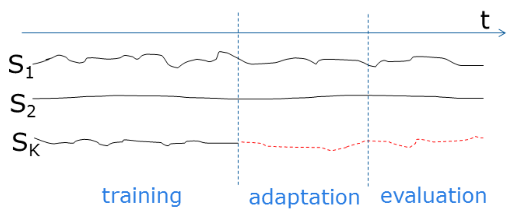
- All sensors generate sensor values at fixed time intervals, and sensor values are temporally aligned.
- Sensor values start at time 1. At time , sensors are replaced by new sensors ( corresponds to sensor failure). We have sensor values until time .
- There is only a single change point, i.e., time , and it is already given.
3. Approach
3.1. Assumptions and Intuition
- Sensor values from the reference sensors are correlated with those from the replaced sensors.
- Sensor values from the reference sensors are correlated with those from the new sensors.
3.2. Formulation
3.3. Optimization
3.4. Initialization
3.5. Parameter Tuning
4. Empirical Study
- Weather Data: the dataset consisted of weather sensor data collected from Weather Underground (https://www.wunderground.com/, accessed on 17 May 2021). The dataset involved a number of personal weather stations; and each station (compound sensor) contains a set of individual sensors including temperature, dew point, humidity, wind speed, wind gust, pressure, etc. These weather stations were selected from a set of clusters/regions (e.g., Los Angeles, San Francisco, Austin, Chicago, etc.), each with three stations. The clusters were determined based on the cities in which the stations are located. Stations within a cluster tended to produce more similar sensor values than those across clusters. Sensor values were sampled every 5 or 10 min. We temporally aligned sensor values as a preprocessing step. The data used in our empirical study are available for download (https://github.com/usc-isi-i2/sensor-adaptation/tree/master/datasets/weather/dataset, accessed on 17 May 2021). The data were organized into different geographical clusters where each cluster contains a few weather stations. Sensor values were represented in JSON format where each attribute corresponded to a different sensor type.
- UUV Data: the dataset was collected by letting a UUV travel from a starting point to an end point in a simulated environment. The UUV contained a propeller RPM sensor, a waterspeed sensor, and a compound sensor called Doppler Velocity Log (DVL) sensor. The DVL sensor consisted of seven individual sensors including surge, heave, sway, pitch, roll, depth, and heading. Figure 4 shows the locations of these sensors on a UUV. Each sensor produced a sensor value every second. We simulated 20 trips and collected sensor values at each second. The trajectory of the UUV varies in each trip due to different starting/end points and water currents. The total number of samples in each trip varied between 500 and 2000.

- Replace: non-adaptation method that substitutes each replaced sensor with a new sensor that has the closest mean and variance in sensor values.
- Refer: adaptation method that reconstructs sensor values of replaced sensors using reference sensors, without exploiting any new sensor.
- ReferZ: adaptation method that works in the following three steps:
- Learn a regression model on the target domain to reconstruct the new sensors from reference sensors.
- Use the learned regression model to reconstruct the new sensors on the source domain.
- Learn a reconstruction function on the source domain to reconstruct replaced sensors from reference sensors and reconstructed new sensors.
4.1. Results on Weather Data
4.2. Results on UUV Data
4.3. Evaluation in BRASS Project
5. Extensions
5.1. Estimating Adaptation Quality
- Find its nearest neighbors in the source domain according to distances defined in Equation (3).
- Compute the standard deviation on the given reconstructed sensor value among the neighbors found in Step 1.
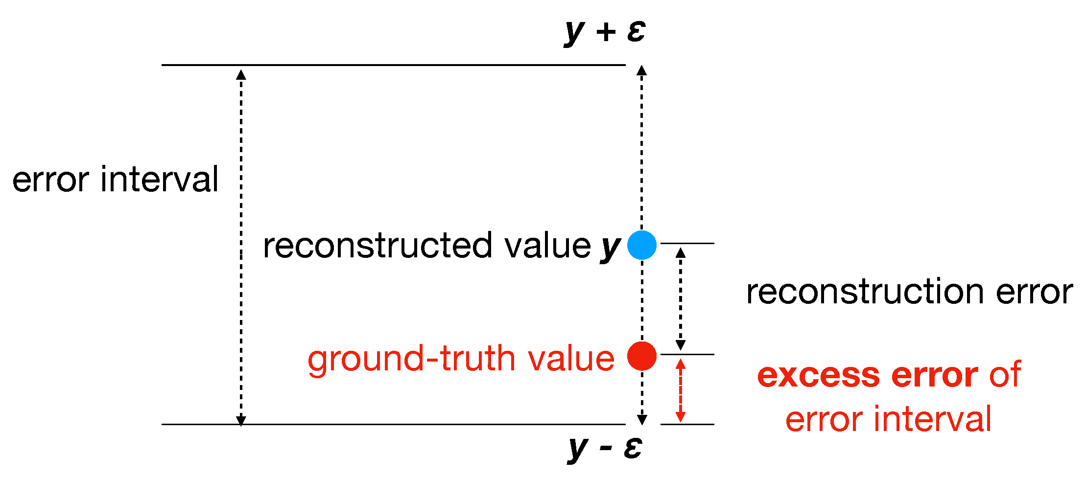
- Set the estimated error interval to be , where is a scaling factor. An ideal makes the error interval as tight as possible. can be tuned on source-domain samples by optimizing the “excess error” notion defined below.
5.2. Ability to Exploit Many Sensors
- Noisy sensors are likely to be involved and can degrade adaptation performance. For example, if some reference sensors produce highly noisy values, the nearest neighbor distances can suffer from the noise. Additionally, noisy values in reference or new sensors can cause the optimization algorithm to get stuck in poor local minima.
- A large number of sensors leads to a large parameter space of , which significantly increases the computational cost of the adaptation algorithm.
- Selecting a subset of reference sensors: For each reference sensor, compute the average correlation between its sensor values and those from each replaced sensor, and then select reference sensors with the largest average correlation scores.
- Selecting a subset of new sensors: For each new sensor, compute the average correlation between its sensor values and those from each replaced sensor as well as each selected reference sensor in Step 1, and then select new sensors with the largest average correlation scores.
5.3. Empirical Study
6. Related Work
7. Conclusions
Author Contributions
Funding
Data Availability Statement
Acknowledgments
Conflicts of Interest
References
- Hughes, J.; Sparks, C.; Stoughton, A.; Parikh, R.; Reuther, A.; Jagannathan, S. Building Resource Adaptive Software Systems (BRASS): Objectives and System Evaluation. ACM SIGSOFT Softw. Eng. Notes 2016, 41, 1–2. [Google Scholar] [CrossRef]
- Dereszynski, E.W.; Dietterich, T.G. Probabilistic Models for Anomaly Detection in Remote Sensor Data Streams. arXiv 2012, arXiv:1206.5250. [Google Scholar]
- Dereszynski, E.W.; Dietterich, T.G. Spatiotemporal Models for Data-Anomaly Detection in Dynamic Environmental Monitoring Campaigns. ACM Trans. Sens. Netw. TOSN 2011, 8, 3. [Google Scholar] [CrossRef]
- Gubbi, J.; Buyya, R.; Marusic, S.; Palaniswami, M. Internet of Things (IoT): A Vision, Architectural Elements, and Future Directions. Future Gener. Comput. Syst. 2013, 29, 1645–1660. [Google Scholar] [CrossRef]
- Tong, B.; Wang, G.; Zhang, W.; Wang, C. Node Reclamation and Replacement for Long-Lived Sensor Networks. IEEE Trans. Parallel Distrib. Syst. 2011, 22, 1550–1563. [Google Scholar] [CrossRef]
- Lai, T.T.T.; Chen, W.J.; Li, K.H.; Huang, P.; Chu, H.H. Triopusnet: Automating Wireless Sensor Network Deployment and Replacement in Pipeline Monitoring. In Proceedings of the 11th International Conference on Information Processing in Sensor Networks, Beijing, China, 16–19 April 2012; pp. 61–72. [Google Scholar]
- Basseville, M.; Nikiforov, I.V. Detection of Abrupt Changes: Theory and Application; Prentice Hall Englewood Cliffs: Hoboken, NJ, USA, 1993; Volume 104. [Google Scholar]
- Gustafsson, F.; Gustafsson, F. Adaptive Filtering and Change Detection; Wiley: New York, NY, USA, 2000; Volume 1. [Google Scholar]
- Brodsky, E.; Darkhovsky, B.S. Nonparametric Methods in Change Point Problems; Springer Science & Business Media: Berlin/Heidelberg, Germany, 2013; Volume 243. [Google Scholar]
- Aminikhanghahi, S.; Cook, D.J. A Survey of Methods for Time Series Change Point Detection. Knowl. Inf. Syst. 2016, 51, 1–29. [Google Scholar] [CrossRef]
- Dietterich, T.G.; Dereszynski, E.W.; Hutchinson, R.A.; Sheldon, D.R. Machine Learning for Computational Sustainability. In Proceedings of the International Green Computing Conference, San Jose, CA, USA, 4–8 June 2012. [Google Scholar]
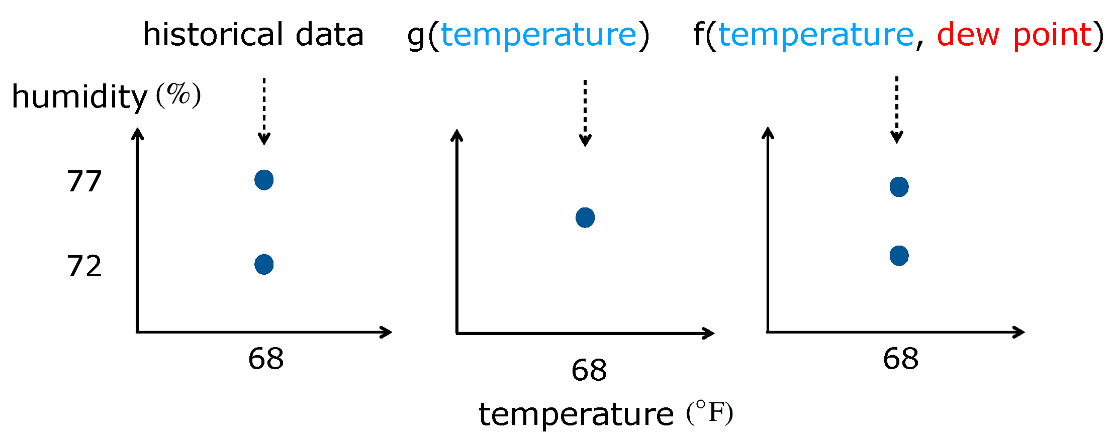
- Lawrence, M.G. The Relationship Between Relative Humidity and the Dewpoint Temperature in Moist Air: A Simple Conversion and Applications. Bull. Am. Meteorol. Soc. 2005, 86, 225–233. [Google Scholar] [CrossRef]
- Friedman, J.; Hastie, T.; Tibshirani, R. The Elements of Statistical Learning; Springer Series in Statistics; Springer: Berlin/Heidelberg, Germany, 2001; Volume 1. [Google Scholar]
- Shi, Y. Learning to Adapt to Sensor Changes and Failures. Ph.D. Thesis, Computer Science Department, University of Southern California, Los Angeles, CA, USA, 2019. [Google Scholar]
- Pan, S.J.; Yang, Q. A Survey on Transfer Learning. IEEE Trans. Knowl. Data Eng. 2010, 22, 1345–1359. [Google Scholar] [CrossRef]
- Elnahrawy, E.; Nath, B. Context-Aware Sensors. In European Workshop on Wireless Sensor Networks; Springer: Berlin/Heidelberg, Germany, 2004; pp. 77–93. [Google Scholar]
- Pimentel, M.A.; Clifton, D.A.; Clifton, L.; Tarassenko, L. A Review of Novelty Detection. Signal Process. 2014, 99, 215–249. [Google Scholar] [CrossRef]
- Reddy, S.; Mun, M.; Burke, J.; Estrin, D.; Hansen, M.; Srivastava, M. Using Mobile Phones to Determine Transportation Modes. ACM Trans. Sens. Netw. TOSN 2010, 6, 13. [Google Scholar] [CrossRef]
- Zheng, Y.; Liu, L.; Wang, L.; Xie, X. Learning Transportation Mode from Raw GPS Data for Geographic Applications on the Web. In Proceedings of the 17th International Conference on World Wide Web, Beijing, China, 21–25 April 2008; pp. 247–256. [Google Scholar]
- Cleland, I.; Han, M.; Nugent, C.; Lee, H.; McClean, S.; Zhang, S.; Lee, S. Evaluation of Prompted Annotation of Activity Data Recorded from a Smart Phone. Sensors 2014, 14, 15861–15879. [Google Scholar] [CrossRef]
- Han, M.; Vinh, L.T.; Lee, Y.K.; Lee, S. Comprehensive Context Recognizer Based on Multimodal Sensors in a Smartphone. Sensors 2012, 12, 12588–12605. [Google Scholar] [CrossRef]
- Harchaoui, Z.; Moulines, E.; Bach, F.R. Kernel Change-Point Analysis. In Proceedings of the 21st International Conference on Neural Information Processing Systems, Vancouver, BC, Canada, 8–11 December 2008; pp. 609–616. [Google Scholar]
- Idé, T.; Tsuda, K. Change-Point Detection Using Krylov Subspace Learning. In Proceedings of the 2007 SIAM International Conference on Data Mining, Minneapolis, MN, USA, 26–28 April 2007; pp. 515–520. [Google Scholar]
- Moskvina, V.; Zhigljavsky, A. An Algorithm Based on Singular Spectrum Analysis for Change-Point Detection. Commun. Stat. Simul. Comput. 2003, 32, 319–352. [Google Scholar] [CrossRef]
- Saatçi, Y.; Turner, R.D.; Rasmussen, C.E. Gaussian Process Change Point Models. In Proceedings of the 27th International Conference on Machine Learning (ICML-10), Haifa, Israel, 21–24 June 2010; pp. 927–934. [Google Scholar]
- Angiulli, F.; Pizzuti, C. Fast Outlier Detection in High Dimensional Spaces. In Proceedings of the 6th European Conference on Principles of Data Mining and Knowledge Discovery, Helsinki, Finland, 19–23 August 2002; pp. 15–27. [Google Scholar]
- Chen, H.; Zhang, N. Graph-Based Change-Point Detection. Ann. Stat. 2015, 43, 139–176. [Google Scholar] [CrossRef]
- Neema, S.; Parikh, R.; Jagannathan, S. Building Resource Adaptive Software Systems. IEEE Softw. 2019, 36, 103–109. [Google Scholar] [CrossRef]
- Grosse-Puppendahl, T.; Berlin, E.; Borazio, M. Enhancing Accelerometer-Based Activity Recognition with Capacitive Proximity Sensing. In International Joint Conference on Ambient Intelligence; Springer: Berlin/Heidelberg, Germany, 2012; pp. 17–32. [Google Scholar]
- Chen, C.; Jafari, R.; Kehtarnavaz, N. Improving Human Action Recognition Using Fusion of Depth Camera and Inertial Sensors. IEEE Trans. Hum. Mach. Syst. 2014, 45, 51–61. [Google Scholar] [CrossRef]
- Hu, C.; Chen, Y.; Peng, X.; Yu, H.; Gao, C.; Hu, L. A Novel Feature Incremental Learning Method for Sensor-Based Activity Recognition. IEEE Trans. Knowl. Data Eng. 2018, 31, 1038–1050. [Google Scholar] [CrossRef]
- Hou, B.J.; Zhang, L.; Zhou, Z.H. Learning with Feature Evolvable Streams. IEEE Trans. Knowl. Data Eng. 2019. [Google Scholar] [CrossRef]
- Shi, Y.; Knoblock, C. Learning with Previously Unseen Features. In Proceedings of the International Joint Conference on Artificial Intelligence, Melbourne, Australia, 19–25 August 2017. [Google Scholar]
- Kounev, S.; Lewis, P.; Bellman, K.L.; Bencomo, N.; Camara, J.; Diaconescu, A.; Esterle, L.; Geihs, K.; Giese, H.; Götz, S.; et al. The Notion of Self-Aware Computing. In Self-Aware Computing Systems; Springer: Cham, Switzerland, 2017; pp. 3–16. [Google Scholar]
- Esterle, L.; Rinner, B. An Architecture for Self-Aware IoT Applications. In Proceedings of the 2018 IEEE International Conference on Acoustics, Speech and Signal Processing (ICASSP), Calgary, AB, Canada, 15–20 April 2018; pp. 6588–6592. [Google Scholar]
- Möstl, M.; Schlatow, J.; Ernst, R.; Hoffmann, H.; Merchant, A.; Shraer, A. Self-Aware Systems for the Internet-of-Things. In Proceedings of the 2016 International Conference on Hardware/Software Codesign and System Synthesis (CODES + ISSS), Pittsburgh, PA, USA, 2–7 October 2016; pp. 1–9. [Google Scholar]
- Chen, B.W.; Imran, M.; Nasser, N.; Shoaib, M. Self-Aware Autonomous City: From Sensing to Planning. IEEE Commun. Mag. 2019, 57, 33–39. [Google Scholar] [CrossRef]
- Mundhenk, T.N.; Everist, J.; Landauer, C.; Itti, L.; Bellman, K. Distributed Biologically-Based Real-Time Tracking in the Absence of Prior Target Information. In Proceedings of the Intelligent Robots and Computer Vision XXIII: Algorithms, Techniques, and Active Vision, Boston, MA, USA, 23–26 October 2005; Volume 6006. [Google Scholar]
- Landauer, C.; Bellman, K.L. An Architecture for Self-Awareness Experiments. In Proceedings of the 2017 IEEE International Conference on Autonomic Computing (ICAC), Columbus, OH, USA, 17–21 July 2017; pp. 255–262. [Google Scholar]
- Guettatfi, Z.; Hübner, P.; Platzner, M.; Rinner, B. Computational Self-Awareness as Design Approach for Visual Sensor Nodes. In Proceedings of the 2017 12th International Symposium on Reconfigurable Communication-Centric Systems-on-Chip (ReCoSoC), Madrid, Spain, 12–14 July 2017; pp. 1–8. [Google Scholar]
- Esterle, L.; Simonjan, J.; Nebehay, G.; Pflugfelder, R.; Domínguez, G.F.; Rinner, B. Self-Aware Object Tracking in Multi-Camera Networks. In Self-Aware Computing Systems; Springer: Cham, Switzerland, 2016; pp. 261–277. [Google Scholar]
- Salama, M.; Shawish, A.; Bahsoon, R. Dynamic Modelling of Tactics Impact on the Stability of Self-Aware Cloud Architectures. In Proceedings of the 2016 IEEE 9th International Conference on Cloud Computing (CLOUD), San Francisco, CA, USA, 27 June–2 July 2016; pp. 871–875. [Google Scholar]
- Iosup, A.; Zhu, X.; Merchant, A.; Kalyvianaki, E.; Maggio, M.; Spinner, S.; Abdelzaher, T.; Mengshoel, O.; Bouchenak, S. Self-Awareness of Cloud Applications. In Self-Aware Computing Systems; Springer: Cham, Switzerland, 2017; pp. 575–610. [Google Scholar]
- Parashar, M.; Hariri, S. Autonomic Computing: Concepts, Infrastructure, and Applications; CRC Press: Boca Raton, FL, USA, 2018. [Google Scholar]
- Lalanda, P.; McCann, J.A.; Diaconescu, A. Autonomic Computing: Principles, Design and Implementation; Springer Science & Business Media: Berlin/Heidelberg, Germany, 2013. [Google Scholar]
- Abeywickrama, D.B.; Ovaska, E. A Survey of Autonomic Computing Methods in Digital Service Ecosystems. Serv. Oriented Comput. Appl. 2017, 11, 1–31. [Google Scholar] [CrossRef]


| Sensor | Replace | Refer | ReferZ | ASC | Imp. |
|---|---|---|---|---|---|
| temperature | 3.94 ± 0.024 | 0.61 ± 0.011 | 0.59 ± 0.009 | 0.57 ± 0.010 | 4.1 |
| humidity | 5.73 ± 0.023 | 0.72 ± 0.016 | 0.71 ± 0.015 | 0.72 ± 0.015 | −1.7 |
| dew point | 3.89 ± 0.027 | 0.70 ± 0.010 | 0.68 ± 0.009 | 0.67 ± 0.010 | 2.8 |
| wind speed | 8.24 ± 0.084 | 5.20 ± 0.063 | 5.21 ± 0.064 | 5.11 ± 0.060 | 1.7 |
| wind gust | 10.81 ± 0.073 | 6.65 ± 0.052 | 6.65 ± 0.048 | 6.31 ± 0.046 | 5.0 |
| pressure | 7.82 ± 0.16 | 3.42 ± 0.19 | 2.48 ± 0.17 | 1.83 ± 0.17 | 26.2 |
| Sensor | Replace | Refer | ReferZ | ASC | Imp. |
|---|---|---|---|---|---|
| temperature | 3.94 ± 0.024 | 0.73 ± 0.018 | 0.71 ± 0.013 | 0.68 ± 0.014 | 4.2 |
| humidity | 5.73 ± 0.023 | 0.87 ± 0.021 | 0.88 ± 0.020 | 0.87 ± 0.022 | 0 |
| dew point | 3.89 ± 0.027 | 0.75 ± 0.018 | 0.74 ± 0.012 | 0.72 ± 0.011 | 2.6 |
| wind speed | 8.24 ± 0.084 | 6.07 ± 0.080 | 6.11 ± 0.074 | 6.13 ± 0.082 | −1.8 |
| wind gust | 10.81 ± 0.073 | 7.24 ± 0.069 | 7.08 ± 0.072 | 6.83 ± 0.070 | 3.5 |
| pressure | 7.82 ± 0.16 | 3.82 ± 0.21 | 2.83 ± 0.20 | 2.26 ± 0.18 | 20.1 |
| Sensor | Replace | Refer | ReferZ | ASC | Imp. |
|---|---|---|---|---|---|
| surge | 2.47 ± 0.14 | 0.66 ± 0.071 | 0.58 ± 0.048 | 0.47 ± 0.051 | 18.9 |
| heave | 0.13 ± 0.0068 | 0.020 ± 0.0062 | 0.020 ± 0.0046 | 0.019 ± 0.0049 | 6.5 |
| sway | 2.31 ± 0.13 | 0.74 ± 0.065 | 0.72 ± 0.059 | 0.71 ± 0.063 | 1.1 |
| Sensor | Replace | Refer | ReferZ | ASC | Imp. |
|---|---|---|---|---|---|
| surge | 2.47 ± 0.14 | 0.71 ± 0.084 | 0.67 ± 0.078 | 0.62 ± 0.081 | 6.0 |
| heave | 0.094 ± 0.0063 | 0.026 ± 0.0073 | 0.026 ± 0.0070 | 0.024 ± 0.0073 | 3.4 |
| sway | 2.31 ± 0.13 | 0.78 ± 0.079 | 0.75 ± 0.080 | 0.75 ± 0.076 | −0.5 |
| Sensor | Success Rate (%) | Imp. |
|---|---|---|
| temperature | 95.4 | 61.6 |
| humidity | 96 | 65.8 |
| dew point | 100 | 71.1 |
| wind speed | 84.6 | 28.7 |
| wind gust | 66.7 | 24.0 |
| Replaced Sensor | Reconstruction Error | Excess Error | ||
|---|---|---|---|---|
| ASC | ASC | ASC | ASC | |
| temperature (F) | 0.47 ± 0.012 | 0.38 ± 0.009 | 0.34 ± 0.010 | 0.22 ± 0.009 |
| humidity (%) | 0.53 ± 0.016 | 0.47 ± 0.014 | 0.42 ± 0.014 | 0.31 ± 0.011 |
| dew point (F) | 0.47 ± 0.012 | 0.44 ± 0.009 | 0.37 ± 0.010 | 0.25 ± 0.009 |
| wind speed (mph) | 5.04 ± 0.061 | 4.83 ± 0.059 | 4.36 ± 0.052 | 3.71 ± 0.055 |
| wind gust (mph) | 6.28 ± 0.052 | 5.61 ± 0.045 | 4.75 ± 0.041 | 3.96 ± 0.042 |
| pressure (Pa) | 3.17 ± 0.19 | 1.68 ± 0.18 | 2.68 ± 0.19 | 1.04 ± 0.18 |
Publisher’s Note: MDPI stays neutral with regard to jurisdictional claims in published maps and institutional affiliations. |
© 2021 by the authors. Licensee MDPI, Basel, Switzerland. This article is an open access article distributed under the terms and conditions of the Creative Commons Attribution (CC BY) license (https://creativecommons.org/licenses/by/4.0/).
Share and Cite
Shi, Y.; Li, A.; Kumar, T.K.S.; Knoblock, C.A. Building Survivable Software Systems by Automatically Adapting to Sensor Changes. Appl. Sci. 2021, 11, 4808. https://doi.org/10.3390/app11114808
Shi Y, Li A, Kumar TKS, Knoblock CA. Building Survivable Software Systems by Automatically Adapting to Sensor Changes. Applied Sciences. 2021; 11(11):4808. https://doi.org/10.3390/app11114808
Chicago/Turabian StyleShi, Yuan, Ang Li, T. K. Satish Kumar, and Craig A. Knoblock. 2021. "Building Survivable Software Systems by Automatically Adapting to Sensor Changes" Applied Sciences 11, no. 11: 4808. https://doi.org/10.3390/app11114808
APA StyleShi, Y., Li, A., Kumar, T. K. S., & Knoblock, C. A. (2021). Building Survivable Software Systems by Automatically Adapting to Sensor Changes. Applied Sciences, 11(11), 4808. https://doi.org/10.3390/app11114808