Image Denoising Using a Novel Deep Generative Network with Multiple Target Images and Adaptive Termination Condition

Abstract

Image denoising, a classic ill-posed problem, aims to recover a latent image from a noisy measurement. Over the past few decades, a considerable number of denoising methods have been studied extensively. Among these methods, supervised deep convolutional networks have garnered increasing attention, and their superior performance is attributed to their capability to learn realistic image priors from a large amount of paired noisy and clean images. However, if the image to be denoised is significantly different from the training images, it could lead to inferior results, and the networks may even produce hallucinations by using inappropriate image priors to handle an unseen noisy image. Recently, deep image prior (DIP) was proposed, and it overcame this drawback to some extent. The structure of the DIP generator network is capable of capturing the low-level statistics of a natural image using an unsupervised method with no training images other than the image itself. Compared with a supervised denoising model, the unsupervised DIP is more flexible when processing image content that must be denoised. Nevertheless, the denoising performance of DIP is usually inferior to the current supervised learning-based methods using deep convolutional networks, and it is susceptible to the over-fitting problem. To solve these problems, we propose a novel deep generative network with multiple target images and an adaptive termination condition. Specifically, we utilized mainstream denoising methods to generate two clear target images to be used with the original noisy image, enabling better guidance during the convergence process and improving the convergence speed. Moreover, we adopted the noise level estimation (NLE) technique to set a more reasonable adaptive termination condition, which can effectively solve the problem of over-fitting. Extensive experiments demonstrated that, according to the denoising results, the proposed approach significantly outperforms the original DIP method in tests on different databases. Specifically, the average peak signal-to-noise ratio (PSNR) performance of our proposed method on four databases at different noise levels is increased by 1.90 to 4.86 dB compared to the original DIP method. Moreover, our method achieves superior performance against state-of-the-art methods in terms of popular metrics, which include the structural similarity index (SSIM) and feature similarity index measurement (FSIM). Thus, the proposed method lays a good foundation for subsequent image processing tasks, such as target detection and super-resolution.

1. Introduction

During acquisition and transmission, the quality of digital images inevitably degrades owing to corruption caused by various reasons. Therefore, the ability to recover a clean image from a noisy one is of great importance, and image denoising is a fundamental step applied in all image processing pipelines. In the computer vision field, image denoising has been a research hotspot since the 1990s. After decades of research, many denoising algorithms had achieved good results through approaches such as non-local self-similarity in natural images [1,2,3], low rankness-based models [4,5], sparse representation-based models [3,6,7], and fuzzy (or neuro-fuzzy)-based models [8,9]. Nevertheless, researchers are still aiming to further improve the performance of image denoising algorithms.

Existing denoising algorithms can be roughly divided into internal algorithms and external algorithms [10]. Internal algorithms utilize the noisy image itself, while the external algorithms exploit clean, natural images related to the noisy image. Internal image denoising algorithms include filter algorithms, low rankness-based models, and sparse representation-based algorithms. Representative examples of filter algorithms are the non-local means (NLM) algorithm and the block-matching and 3D filtering (BM3D) algorithm. The NLM algorithm [1], proposed by Baudea et al. in 2005, exploited non-local self-similarity in natural images. It first finds similar patches and obtains their weighted average to achieve the denoised patches. Although it exhibits excellent performance, the NLM algorithm is limited by its inability to identify truly similar patches in a noisy environment. BM3D [2], a benchmark denoising algorithm, starts with the block-matching of each reference block, and obtains 3D arrays by grouping similar blocks together. The authors used a two-step algorithm to denoise an image. First, they denoised the input image simply and obtained a basic estimate; next, they achieved an improved denoising effect through collaborative filtering of the basic estimate. Among low rankness-based methods, nuclear norm minimization (NNM) and weighted nuclear norm minimization (WNNM) are two well-known algorithms. The NNM algorithm [4] was proposed by Ji et al. for video denoising. In their work, the problem of removing noise was transformed into a low-rank matrix completion problem, which can be well solved by singular value decomposition. However, the authors equalized each singular value to ensure the convexity of the objective function, which severely restricts its capability and flexibility when dealing with denoising problems. Based on the NMM algorithm and proposed in [5], the WNNM algorithm takes advantage of the non-local self-similarity of the image for denoising. Among sparse representation-based algorithms, the K-singular value decomposition (K-SVD) algorithm, the learned simultaneous sparse coding (LSSC) algorithm, and the non-locally centralized sparse representation (NCSR) algorithm are three noteworthy algorithms. K-SVD [6] is a classic dictionary learning algorithm, which utilizes the sparsity and redundancy of over-complete learning dictionaries to produce high-quality denoising images. LSSC [3] exploits the combination of the self-similarity of image patches and sparse coding to further boost denoising performance. The NCSR [7] algorithm was proposed by Dong et al. and utilizes non-local self-similarity and sparse representation of images. It introduces the concept of sparse coding noise with the goal of suppressing the sparse coding noise to denoise an image. In general, most of these traditional denoising methods use custom-made image priority and multiple, manually selected parameters, providing ample room for improvement.

In recent years, deep learning-based methods have become a popular research direction in the field of image denoising. These methods can be categorized as external methods whose denoising performance is superior to internal methods. The main idea is to collect a large number of noise-clean image pairs, and then train the deep neural network denoiser using end-to-end learning. These methods have significant advantages in accumulating knowledge from big datasets; thus, they can achieve superior denoising performance. In 2017, Zhang et al. proposed Deep CNN (DnCNN) [11], which exploited the residual learning strategy to remove noise. They introduced the batch normalization technique as it not only reduced the training time, but also boosted the denoising effect quantitatively and qualitatively. However, it is only effective when the noise level is within a pre-set range. Hence, Zhang et al. proposed FFDNet in [12]. FFDNet showed considerable improvement in flexibility and robustness using a single network. Specifically, it was formulated as $x=F\left(y,M;\Theta \right)$, where x is the expected output, y is the input noise observation, and M is a noise level map. In the DnCNN model $x=F\left(y;\Theta \right)$, the parameters $\Theta$ change with the noise level. As for the FFDNet model, M is modeled as the input and the hyper-parameters have no relationship to the noise level. Therefore, it could handle different noise levels in a flexible manner using a single network. The consensus neural network (CsNet) was proposed by Choi et al. [13], and combines multiple relatively weak image denoisers to produce a satisfactory result. CsNet exhibits superior performance in three aspects: solving the noise level mismatch, incorporating denoisers for different image classes, and uniting different denoiser types. In summary, these supervised denoising networks are exceedingly effective when supplied with plenty of noise-clean image pairs for training, but collecting clean images of the ground truth in many real-world scenarios is very difficult. Moreover, if the image priors are significantly different from the image to be denoised, the supervised denoising networks tend to produce hallucination-like effects when handling an unseen noisy image, because the previously learned image statistics cannot handle the untouched image content and noise level well. These networks have strong data dependence [14], leading to a lack of flexibility.

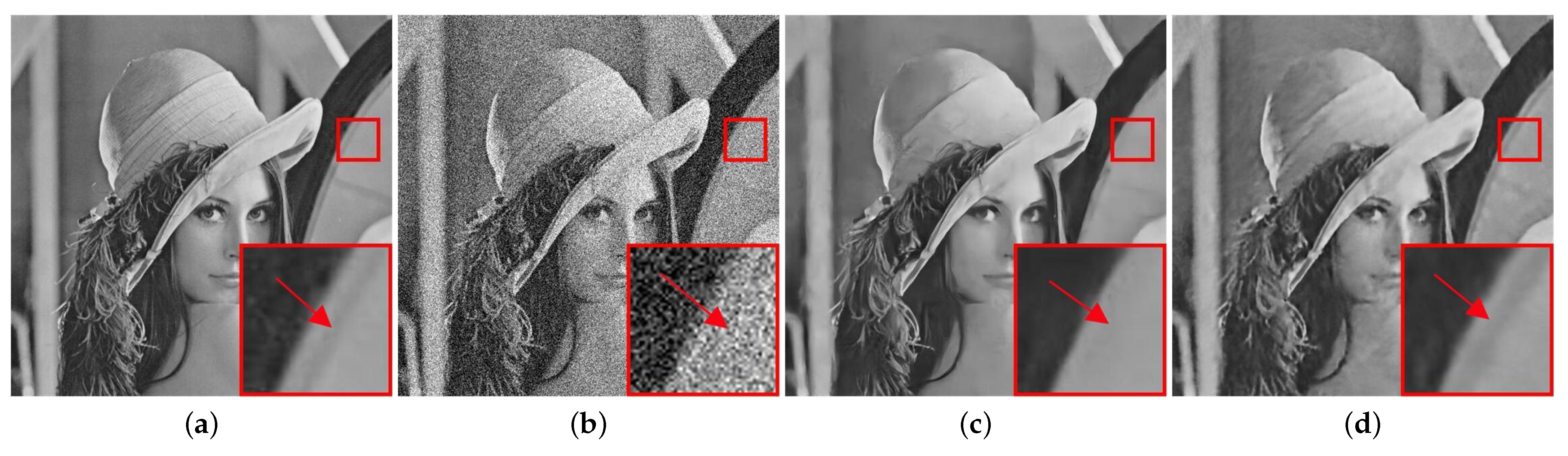
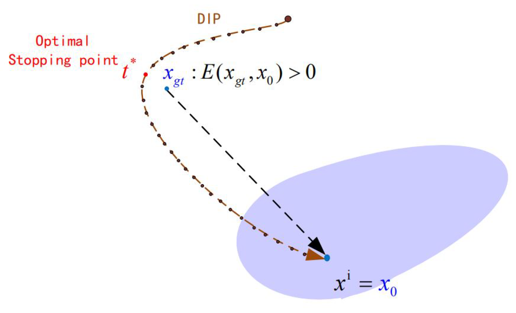
To overcome the aforementioned limitations, researchers have focused on training unsupervised denoising networks without training images. Recently, research on generative networks using the deep image prior (DIP) framework [15] demonstrated that even if only the input image itself is used in training, deep convolutional neural networks (CNNs) can still provide superior performance on various inverse problems. No prior training is required, and random noise is used as the network input to generate denoised images. It can be widely used in image noise reduction, super-resolution, and other image restoration problems. Because the hyper-parameters of DIP are determined based on the specific noisy image, it may, in some cases, achieve better denoising results than the supervised denoising models. 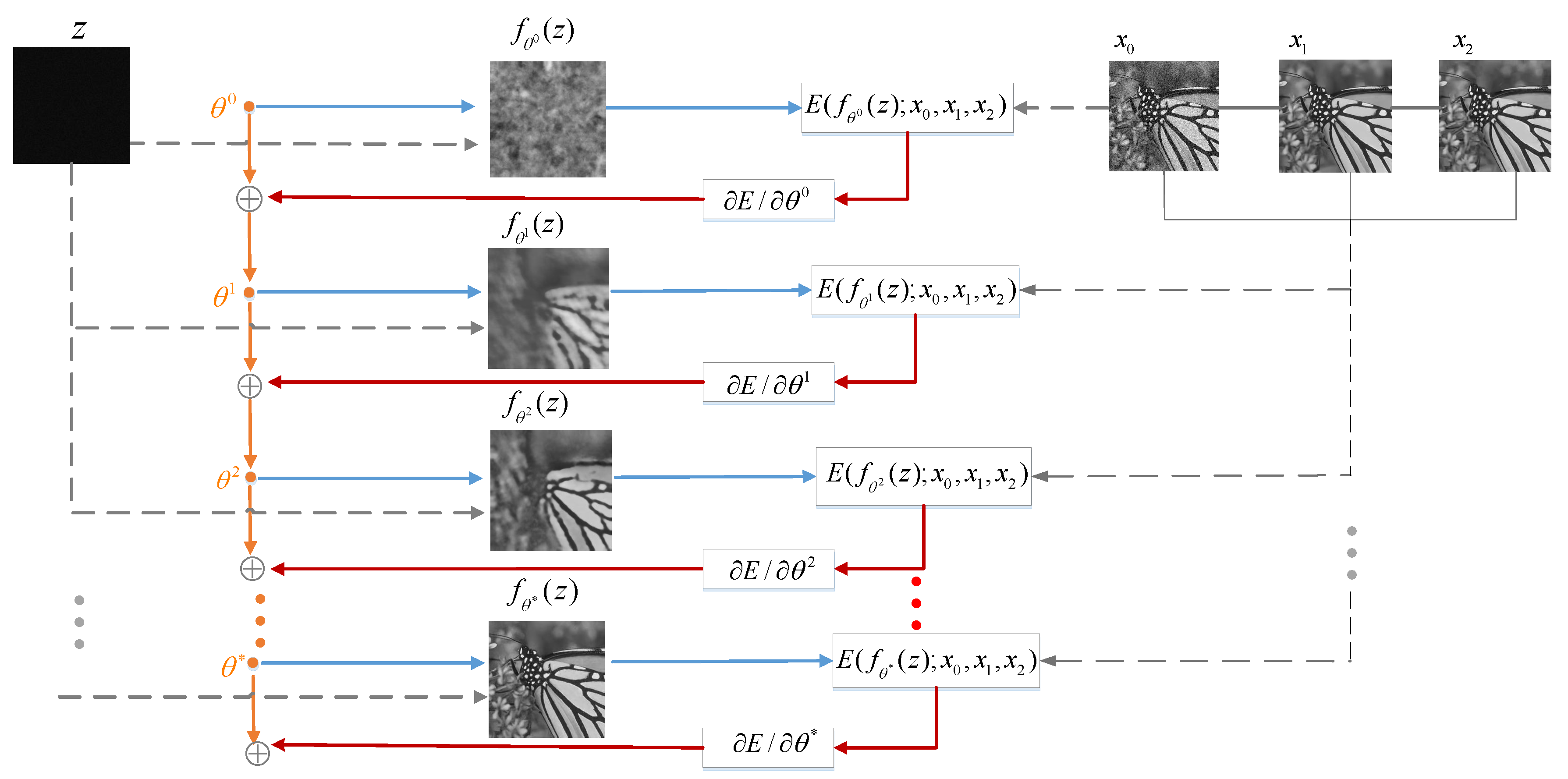As shown in Figure 1, although the general denoising performance of DIP is inferior to that of DnCNN, we can still find some local details, such as the magnified part of the images, that DIP can preserve more accurately as compared with DnCNN. The reason is that the prior knowledge captured by DnCNN cannot handle the subtle information that DIP can. DIP performs the inference by stopping the training early. However, in the original DIP model, the early stopping point is set as a fixed number of iterations using experimental data, so the result is not always optimal. Furthermore, the noisy image is used as the target image that provides poor guidance and leads to slow convergence of the generative network. Thus, the denoising performance of DIP is much lower than that of deep learning in some cases, and it still leaves room for improvement. In view of the limitations of the existing DIP method, we propose a novel deep generative network with multiple target images and an adaptive termination condition, which not only retains the flexibility of the original DIP model, but also improves denoising performance. Specifically, instead of the noisy image, we use two target images of higher quality to participate in the formation of the loss functions. In addition, we adopt a noise level estimation (NLE) method to automatically terminate the iterative process to resolve the early stopping problem, prevent over-fitting, and ensure an optimal output image.

The remainder of the paper is organized as follows: Section 2 introduces a literature review of related work. In Section 3, we describe the proposed approach in detail. Section 4 discusses our experimental results and analysis. We discuss our current work and future work in Section 5. Finally, we conclude this paper in Section 6.

2. Related Work

2.1. Background

Image denoising is the most fundamental inverse problem of image processing, and its purpose is to recover the underlying image from its noisy measurement. In most cases, image denoising is an ill-posed problem; based on the noisy observation, we can always find many reasonable images that could belong to the clean image manifold. The image denoising problem can be described by a simple mathematical formula:

$$y=x+n$$

(1)

where y is a noisy observed image and x is a clean, no-noise image. Generally, n is assumed to be the additive white Gaussian noise (AWGN), which is widely used in the field of image denoising. The denoising problem requires finding the denoised image $\widehat{x}$ that is closest to the true value image.

2.2. Deep Neural Network with Training Pairs

A deep neural network with training pairs is a type of supervised learning method that requires training on large datasets. It aims to map a noisy image to a clean manifold to enable it to remove noise once it is trained. When a large number of training pairs are usable, a neural network can be trained in the following manner:

$$\widehat{\theta }=argmi{n}_{\theta }\sum _i\Vert x_{label}^i-f\left(\theta ,x_{noise}^i\right)\Vert$$

(2)

where $\theta \in {\mathbb{R}}^L$ represents the trainable variables, $f:{\mathbb{R}}^N\to {\mathbb{R}}^N$ indicates the neural network, $x_{label}^i\in {\mathbb{R}}^N$ denotes the $i_{th}$ training label, and $x_{noise}^i\in {\mathbb{R}}^N$ is the network input for the $i_{th}$ training pair. In CNN, $\theta$ contains convolution filters and bias terms for all layers. Once trained, the network can be applied to image denoising [16,17,18,19]. Compared with traditional denoising methods such BM3D, WNNM, and NLM, the deep learning-based methods show superior denoising performance by restoring more image details. These supervised deep learning-based methods require a large number of training pairs to learn network hyper-parameters. These parameters, denoted by $\theta$, have a strong data dependence [14]; specifically, when the image content and noise level values are not uniformly distributed in the image database, the denoising results will be poor. Once the training model is determined, the parameters will not change during the test stage. Therefore, when a noisy image is noticeably different from the training images, the neural network may produce non-existent reconstructed output that results in poor denoising performance.

2.3. Deep Image Prior

Different from supervised deep learning-based methods, DIP is regarded as an unsupervised learning method, which does not require a dataset with a large number of clean target images for training. The general idea is similar to the adaptive dictionary learning method. Ulyanov et al. [15] demonstrated that untrained networks can capture some low-level statistics of natural images, especially the translation invariance of local convolution and its usage. A series of such operators can capture pixel neighborhoods on multiple scales. Let $x_0\in {\mathbb{R}}^N$ be a distorted image, and the training process can be characterized as:

$$\widehat{\theta }=argmi{n}_{\theta }\Vert x_0-f\left(\theta ,z\right)\Vert ,\widehat{x}=f\left(\widehat{\theta },z\right)$$

(3)

where the network input $z\in {\mathbb{R}}^M$ is random noise, and $\widehat{x}\in {\mathbb{R}}^N$ is the denoised image output. The U-Net’s encoder-decoder architecture [20] is mainly used by the network, where z is a fixed 3D tensor having the same space size as x and 32 feature maps. The network has a large number of parameters. Specifically, the encoder portion is a contracting path containing maximum pooling layers and stacked convolution, while the decoder portion is an expanding path containing the nearest neighbor upsampling and bilinear upsampling techniques. The encoder is composed of four downsampling layers and four convolutional blocks, while the decoder contains four upsampling layers and four convolutional blocks. No training pair is required, and $f\left(\theta ,z\right)$ is updated at the start. Given the noisy target $x_0$, the denoised image $\widehat{x}$ is acquired by minimizing the reconstruction error $\Vert x_0-f\left(\theta ,z\right)\Vert$ over z and $\theta$. The method starts with the initial values of z with zero-mean Gaussian distribution, and $\theta$ is optimized by gradient descent.

Figure 2 schematically depicts the use of DIP with a fixed number of iterations in the optimization process. Here, Ulyanov et al. optimized Equation (3) by using a data term such as the $L^2$ distance, which compared the generated image with $x_0$:

$$E\left(x;x_0\right)={\parallel x-x_0\parallel }^2$$

(4)

The ground truth value $x_{gt}$ has the non-zero cost $E\left(x_{gt},x_0\right)>0$. As shown in Figure 2, if it runs for a long enough time, DIP will obtain a solution ($x^i=x_0$) that is quite far from $x_{gt}$. However, the optimized path will usually be close to $x_{gt}$, and the early stopping point (here at step $t^{*}$) will obtain a good solution. Ulyanov et al. [15] showed that this prior is comparable to state-of-the-art learning-free methods in image denoising such as BM3D [2]. The prior encodes the hierarchical self-similarity utilized by dictionary-based methods [21] and non-native technologies (such as BM3D). Several layered networks with skipped connections are used for denoising, which plays a vital role in the network architecture.

2.4. Drawbacks of DIP

Despite the flexibility of DIP shown in image denoising, its results are in some cases not optimal. First, the generators used for DIP are usually over-parameterized; that is, the number of network parameters is greater than the number of output dimensions, and too many iterations result in an empirically overfitted image. In Figure 3, it can be seen that for each curve, the peak signal-to-noise ratio (PSNR) result continuously improves until it reaches a specific iteration; beyond this iteration, the resultant curve of PSNR begins to decline. Thus, if the iteration process does not stop at the appropriate iteration, the DIP experiences under- or over-fitting problems. Though Ulyanov et al. set a fixed number of iterations (early stopping point) in the deep natural network, it was based on experimental data; thus, it could not guarantee the optimal denoising effect. As shown in Figure 3, regardless of where the iterations end, not all three output images could achieve the optimal denoising effect at the same iteration due to differences in their optimal early stopping points.

Second, according to the data listed in

Table 1. PNSR(dB) results of DIP and FFDNet on 10 commonly used images with noise level $\sigma$ = 30 and 40.

Images	Barbara	Boat	Cameraman	Couple	Hill	House	Lena	Man	Monarch	Peppers
Noise Level	$\sigma$ = 30
DIP	25.76	28.14	27.31	27.73	28.36	31.04	30.80	28.03	27.91	28.50
FFDNet	28.95	29.66	29.07	29.46	29.57	32.54	32.05	29.35	28.95	29.63
Noise Level	$\sigma$ = 40
DIP	24.26	26.91	25.69	26.28	27.35	29.43	29.43	26.95	26.48	27.13
FFDNet	27.54	28.41	27.82	28.15	28.50	31.40	30.80	28.19	27.70	28.34

, the denoising effect of DIP is inferior to that of the mainstream FFDNet method. The main reason is that DIP’s loss function is defined as:

$$Los{s}_1=MSE\left({\widehat{x}}^i,x_0\right)$$

(5)

where MSE is the mean square error, ${\widehat{x}}^i$ is the output image of the deep neural network, and $x_0$ is the noisy image. The guiding ability of the noisy image $x_0$, which controls the final convergence direction of the output image, is limited. Notably, more noise in the noisy image will weaken its guiding ability, causing slow iteration convergence and poor denoising performance.

3. Methodology

3.1. Multiple Target Images

First, we considered a new approach to enhance the guidance of the loss function described in Equation (5) by adding two sub-items. In other words, we added two images with higher guiding ability (higher image quality) to participate in the calculation of the loss function. Specifically, we applied two mainstream denoising methods (FFDNet and BM3D) to denoise each noisy image, thereby obtaining two preliminary denoised images $x_1$ and $x_2$. Next, we added the MSE values of the two preliminary denoised images ($x_1$ and $x_2$) to the loss function. The new loss function can be computed with:

$$Los{s}_2=MSE\left({\widehat{x}}^i,x_0\right)+MSE\left({\widehat{x}}^i,x_1\right)+MSE\left({\widehat{x}}^i,x_2\right)$$

(6)

where ${\widehat{x}}^i$ is the output image of the network, $x_0$ represents the noisy image, and $x_1$ and $x_2$ are the preliminary denoised images produced by FFDNet and BM3D, respectively. As shown in Figure 4, the proposed approach starts with random weights ${\theta }^0$, and we iteratively update them to minimize the objective function described in Equation (6). For each iteration i, the weights $\theta$ are used to generate the image ${\widehat{x}}^i=f_{{\theta }^i}\left(z\right)$, where the mapping f is a neural network with parameters ${\theta }^i$ and z is a fixed tensor. The image ${\widehat{x}}^i$ is used to calculate the non-zero cost $E\left({\widehat{x}}^i;x_0,x_1,x_2\right)$. The weight ${\theta }^i$ is then updated using the stochastic gradient descent (SGD) training method. The advantage of this method is that it utilizes preliminary denoising images to construct the loss function and can thereby adjust the evolution direction of the generative network model. This ensures that the network output image ${\widehat{x}}^i$ evolves in a reasonable direction within the solution space (close to the ground truth $x_{gt}$). The schematic diagram in Figure 5 shows the center of gravity of $x_0$, $x_1$, and $x_2$, and shows the point ${\overline{x}}_0$, where the network output image ${\widehat{x}}^i$ finally converges in the solution space after adopting the new hybrid loss function. This results in an output image ${\widehat{x}}^i$ that is closer to the undistorted image $x_{gt}$ after a specific iteration. It should be noted that the preliminary denoised image $x_1$ is obtained from FFDNet, which utilizes external information captured through a training image set, while $x_2$ is obtained from BM3D, which utilizes the internal self-similarity information of the image. Consequently, the proposed method essentially utilizes both the internal and external prior constraints of the image to remove noise.

3.2. Adaptive Termination Condition

Second, to solve the problem of over- or under-fitting, we adopted the previously proposed NLE module [22], which can assess the severity of the noise interference and obtain the noise level value of the noisy image to allow us to set a more reasonable adaptive termination condition. Specifically, the residual image ${\widehat{n}}^i=\left(x_0-{\widehat{x}}^i\right)$ can be obtained by subtracting the $i_{th}$ output image of the deep generative network from the noisy image $x_0$. In the early stages of the network iterations, the network output image ${\widehat{n}}^i$ is far from the undistorted image so the standard deviation $std\left({\widehat{n}}^i\right)$ of the residual image ${\widehat{n}}^i$ is relatively large. When arriving at the appropriate $i_{th}$ iteration, the standard deviation $std\left({\widehat{n}}^i\right)$ of the residual image ${\widehat{n}}^i$ should be close to the noise level value $\sigma$ of the noisy image measured by the previously proposed NLE module. Therefore, $std\left({\widehat{n}}^i\right)\approx \delta$ is used in our work to adaptively terminate the iteration process. In short, with an accurate noise level value, $\sigma$, we can determine when to terminate the iteration process after the appropriate number of iterations has been completed. As shown in Figure 5, the adaptive termination point ${\widehat{x}}_{proposed}^{*}$ of the proposed method is closer to the optimal point $x_{gt}$ than that of the DIP method. Meanwhile, Figure 6 also shows that our adaptive termination condition set the termination step number at 2801, which is very close to the optimal iteration step, 2835, in the iterative process. Thus, the proposed approach can resolve the early stopping problem and achieve more optimal denoising performance.

4. Experiments

4.1. Datasets and Experimental Setup

To evaluate our method comprehensively and verify its effectiveness, we conducted extensive experiments and compared it with DIP and eight other state-of-the-art image denoising methods, including BM3D [2], NCSR [7], WNNM [5], DnCNN [11], FFDNet [12], TWSC [23], RED-Net [24], and CsNet [13]. We conducted denoising experiments on four datasets. In the first dataset, as shown in Figure 7, 10 images commonly used in the literature were selected, comprising six images with a size of 512 × 512 (Barbara, Boat, Couple, Hill, Lena, and Man) and four images with a size of 256 × 256 (Cameraman, House, Monarch, and Peppers). For the second dataset, as illustrated in Figure 8, we randomly selected 50 natural images from the Berkeley segmentation dataset (BSD) [25]. The third dataset contains 10 images obtained randomly from the Flickr1024 database, [26] which consists of 1024 high-quality images covering diverse scenarios. Figure 9 shows some examples. The 10 images in the fourth dataset were randomly selected from Urban100, which contains 100 high-resolution images with various real-world structures; Figure 10 shows some representative images in this dataset.

To test the denoising performance of the proposed method objectively, we utilized three widely accepted image quality evaluation criteria [27,28,29], including PSNR, structural similarity index (SSIM) [30], and the feature similarity index measurement (FSIM) [31]. In addition, we compared the results visually to assess the quality of the denoising effects subjectively. We performed our experiments using a Lenovo desktop with a 4.00 GHz eight-core Intel Core i7-6700K CPU and 16 GB of RAM.

4.2. Experimental Results and Analysis

In this subsection, we present the PSNR results of the proposed method and the original DIP method on 10 commonly used test images.

Table 2. PNSR(dB) results of two methods on 10 commonly used images with various noise levels.

Images	Barbara	Boat	Cameraman	Couple	Hill	House	Lena	Man	Monarch	Peppers
Noise Level	$\sigma$ = 10
DIP	32.06	33.36	32.86	32.97	32.84	35.46	35.36	32.71	33.00	33.77
Proposed	33.79	35.25	35.50	34.80	34.00	37.36	36.97	34.27	35.01	36.44
Noise Level	$\sigma$ = 20
DIP	27.87	30.04	29.35	29.57	29.87	32.68	32.47	29.57	29.68	30.48
Proposed	32.18	32.87	32.01	32.49	32.30	35.01	35.00	32.20	32.24	33.12
Noise Level	$\sigma$ = 30
DIP	25.76	28.14	27.31	27.73	28.36	31.04	30.80	28.03	27.91	28.50
Proposed	30.11	30.91	30.03	30.49	30.62	33.62	33.31	30.31	30.28	31.17
Noise Level	$\sigma$ = 40
DIP	24.26	26.91	25.69	26.28	27.35	29.43	29.43	26.95	26.48	27.13
Proposed	28.29	29.49	28.56	29.11	29.46	32.54	31.95	29.03	28.96	29.69
Noise Level	$\sigma$ = 50
DIP	23.29	25.75	24.52	25.20	26.34	28.51	28.27	26.05	25.37	26.04
Proposed	26.91	28.33	27.49	27.94	28.58	31.48	30.84	28.11	27.88	28.56
Noise Level	$\sigma$ = 60
DIP	22.76	24.96	23.26	24.44	25.49	27.40	27.06	25.23	24.48	24.68
Proposed	25.79	27.44	26.54	27.14	27.82	30.65	30.00	27.36	26.82	27.55

shows the results with noise levels of $\sigma \in$ [10, 20, 30, 40, 50, 60]. The highest PSNR values for each noise level are highlighted in bold. According to the PSNR results shown in Table 2, it can be observed that our approach achieved better performance in all cases compared with the original DIP method. In particular, the processing result of the Barbara image at noise level $\sigma =30$ is notable. Even though the Barbara image has abundant texture details and is complex, our proposed method increased the PSNR result by 4.35 dB. The reason for this is that our proposed method is especially suited to denoising images with complex textures because it utilizes two target images of high quality. Additionally, the minimum increase in the PSNR value was observed on the Hill image with the noise level $\sigma =10$, which reached 1.15 dB. The SSIM and FSIM indexes of the two methods on the 10 commonly used test images were also computed and are shown in

Table 3. SSIM results of two methods on 10 commonly used images with various noise levels.

Images	Barbara	Boat	Cameraman	Couple	Hill	House	Lena	Man	Monarch	Peppers
Noise Level	$\sigma$ = 10
DIP	0.9395	0.9519	0.9570	0.9510	0.9390	0.9600	0.9585	0.9440	0.9512	0.9382
Proposed	0.9630	0.9650	0.9737	0.9648	0.9473	0.9701	0.9742	0.9573	0.9808	0.9784
Noise Level	$\sigma$ = 20
DIP	0.8914	0.9104	0.9170	0.9050	0.8890	0.9400	0.9134	0.8950	0.9039	0.8920
Proposed	0.9527	0.9455	0.9478	0.9452	0.9282	0.9558	0.964	0.9362	0.9663	0.9607
Noise Level	$\sigma$ = 30
DIP	0.8332	0.8741	0.8800	0.8660	0.8540	0.9240	0.8780	0.8590	0.8667	0.8538
Proposed	0.9264	0.9214	0.9238	0.9182	0.9003	0.9468	0.952	0.9063	0.9513	0.9439
Noise Level	$\sigma$ = 40
DIP	0.7696	0.8430	0.8350	0.8240	0.8270	0.9040	0.8440	0.8300	0.8294	0.8270
Proposed	0.8928	0.8971	0.8995	0.8932	0.8755	0.9385	0.9387	0.8803	0.935	0.9262
Noise Level	$\sigma$ = 50
DIP	0.7452	0.8150	0.8100	0.7880	0.8000	0.8900	0.8040	0.8080	0.7940	0.8017
Proposed	0.8576	0.8749	0.8851	0.8678	0.8553	0.9322	0.9265	0.8587	0.9212	0.9078
Noise Level	$\sigma$ = 60
DIP	0.7295	0.7931	0.7640	0.7620	0.7790	0.8780	0.7731	0.7870	0.7637	0.7751
Proposed	0.8238	0.8545	0.8639	0.8474	0.8371	0.9253	0.9154	0.8404	0.9021	0.8958

and

Table 4. FSIM results of two methods on 10 commonly used images with various noise levels.

Images	Barbara	Boat	Cameraman	Couple	Hill	House	Lena	Man	Monarch	Peppers
Noise Level	$\sigma$ = 10
DIP	0.9754	0.9775	0.9511	0.9802	0.9750	0.9520	0.9482	0.9537	0.9765	0.9747
Proposed	0.9825	0.9873	0.9653	0.9868	0.9813	0.9583	0.9857	0.9843	0.9642	0.9668
Noise Level	$\sigma$ = 20
DIP	0.9478	0.9525	0.9249	0.9645	0.9462	0.9262	0.9072	0.9251	0.9490	0.9495
Proposed	0.9760	0.9741	0.9379	0.9739	0.9695	0.9429	0.9767	0.9703	0.9468	0.9472
Noise Level	$\sigma$ = 30
DIP	0.9261	0.9277	0.9024	0.9488	0.9227	0.9065	0.8793	0.9036	0.9256	0.9272
Proposed	0.9630	0.9580	0.9161	0.9574	0.9536	0.9260	0.9671	0.9529	0.9315	0.9312
Noise Level	$\sigma$ = 40
DIP	0.8968	0.9088	0.8809	0.9349	0.9073	0.8912	0.8589	0.8878	0.9045	0.9058
Proposed	0.9501	0.9416	0.8837	0.9398	0.9368	0.9145	0.9567	0.9365	0.9172	0.9168
Noise Level	$\sigma$ = 50
DIP	0.9033	0.8903	0.8633	0.9166	0.8886	0.8735	0.8375	0.8671	0.8826	0.8946
Proposed	0.9377	0.9274	0.8779	0.9237	0.9228	0.9017	0.9459	0.9199	0.9070	0.8900
Noise Level	$\sigma$ = 60
DIP	0.8850	0.8737	0.8494	0.9075	0.8690	0.8615	0.8195	0.8534	0.8654	0.8750
Proposed	0.9249	0.9131	0.8496	0.9112	0.9089	0.8963	0.9373	0.9048	0.8936	0.8899

, respectively. These results show that the proposed method surpassed the DIP method in both SSIM and FSIM, which confirms that our method significantly improved the local structure preservation and global brightness consistency. We also performed experiments to compare the time efficiency of the two methods. In

Table 5. Number of iterations and time(s) of two methods on 10 commonly used images with $\sigma$ = 30.

Images	Barbara	Boat	Cameraman	Couple	Hill	House	Lena	Man	Monarch	Peppers
PSNR	25.76	28.14	27.31	27.73	28.36	31.04	30.80	28.03	27.91	28.50
Number of Iterations
DIP	3373	2505	2083	2555	2774	1551	2687	2655	1703	1575
Proposed	2873	2488	1832	2232	2529	1380	2307	2334	1541	1183
Time
DIP	43.64	31.44	27.09	33.70	37.72	21.97	38.91	39.60	26.11	24.11
Proposed	37.04	31.41	25.00	31.33	36.78	20.75	35.45	37.16	25.44	18.02

, the PSNR value in the second column is the best result that the original DIP method can achieve. The following rows list the number of iterations and time required for DIP and our method to achieve the value, respectively. We can observe that compared with the original DIP method, the proposed method requires less time to reach the PSNR value, which shows that the proposed method surpasses the original DIP method not only in denoising performance but also in time efficiency.

Moreover, we present the average PSNR, SSIM, and FSIM results of the eight other denoising methods on the 10 commonly used images for noise levels $\sigma \in$ [10, 20, 30, 40, 50, 60] in

Table 6. Average PSNR results of different methods on 10 commonly used images with various noise levels.

Method	Noise Level
	$\mathit{\sigma }$ = 10	$\mathit{\sigma }$ = 20	$\mathit{\sigma }$ = 30	$\mathit{\sigma }$ = 40	$\mathit{\sigma }$ = 50	$\mathit{\sigma }$ = 60
BM3D	34.82	31.44	29.59	28.13	27.54	26.37
FFDNet	34.86	31.72	29.95	28.70	27.73	26.92
NCSR	34.81	31.38	29.43	28.06	27.02	26.08
DnCNN	34.94	31.69	29.83	28.52	27.56	26.65
WNNM	35.01	31.61	29.80	28.48	27.51	26.68
RED-Net	34.25	31.13	29.44	28.23	27.26	26.46
TWSC	34.85	31.56	29.73	28.42	27.38	26.51
CsNet	34.62	31.40	29.75	28.55	27.61	26.79
DIP	33.44	30.16	28.36	26.99	25.93	24.98
Proposed	$\mathbf{35.34}$	$\mathbf{32.95}$	$\mathbf{31.08}$	$\mathbf{29.71}$	$\mathbf{28.51}$	$\mathbf{27.71}$

,

Table 7. Average SSIM results of different methods on 10 commonly used images with various noise levels.

Method	Noise Level
	$\mathit{\sigma }$ = 10	$\mathit{\sigma }$ = 20	$\mathit{\sigma }$ = 30	$\mathit{\sigma }$ = 40	$\mathit{\sigma }$ = 50	$\mathit{\sigma }$ = 60
BM3D	0.9306	0.8764	0.8348	0.7968	0.7701	0.7436
FFDNet	0.9330	0.8855	0.8487	0.8177	0.7908	0.7668
NCSR	0.9307	0.8745	0.8289	0.7960	0.7668	0.8603
DnCNN	0.9327	0.8829	0.8432	0.8093	0.7823	0.7523
WNNM	0.9311	0.8773	0.8356	0.8024	0.7779	0.8700
RED-Net	0.9197	0.8694	0.8315	0.7986	0.7698	0.7443
TWSC	0.9313	0.8787	0.8380	0.8035	0.7727	0.7446
CsNet	0.9251	0.8756	0.8405	0.8100	0.7831	0.7581
DIP	0.9490	0.9490	0.8689	0.8333	0.8056	0.7805
Proposed	$\mathbf{0.9675}$	$\mathbf{0.9502}$	$\mathbf{0.9290}$	$\mathbf{0.9077}$	$\mathbf{0.8887}$	$\mathbf{0.8706}$

and

Table 8. Average FSIM results of different methods on 10 commonly used images with various noise levels.

Method	Noise Level
	$\mathit{\sigma }$ = 10	$\mathit{\sigma }$ = 20	$\mathit{\sigma }$ = 30	$\mathit{\sigma }$ = 40	$\mathit{\sigma }$ = 50	$\mathit{\sigma }$ = 60
BM3D	0.9717	0.9452	0.9239	0.9038	0.8883	0.8737
FFDNet	0.9723	0.9476	0.9278	0.9103	0.8947	0.8806
NCSR	0.9719	0.9435	0.9196	0.8956	0.8789	0.7414
DnCNN	0.9720	0.9472	0.9266	0.9078	0.8923	0.8771
WNNM	0.9713	0.9444	0.9233	0.9031	0.8863	0.7508
RED-Net	0.9698	0.9454	0.9251	0.9068	0.8908	0.8770
TWSC	0.9719	0.9448	0.9215	0.9003	0.8815	0.8641
CsNet	0.9718	0.9475	0.9280	0.9099	0.8938	0.8797
DIP	0.9663	0.9393	0.9170	0.8977	0.8817	0.8659
Proposed	$\mathbf{0.9762}$	$\mathbf{0.9615}$	$\mathbf{0.9457}$	$\mathbf{0.9154}$	$\mathbf{0.9154}$	$\mathbf{0.9030}$

, respectively. From Table 6, we can draw the following conclusions. First, although the original DIP method is more flexible, its overall denoising effect is inferior to the mainstream denoising methods. Second, our method surpassed the other mainstream denoising methods and obtained the highest average PSNR results. Specifically, it outperformed the deep learning-based method FFDNet by 0.48 to 1.23 dB. Table 7 shows that the original DIP method was the second best method and achieved impressive SSIM results at noise levels $\sigma \in$ [10, 20, 30, 40, 50]. However, the SSIM results of our method were higher than DIP and improved the SSIM values by 0.0184 to 0.0901. Further, from Table 8, it can be seen that the proposed method also achieved the highest FSIM results in all cases.

To test the robustness of the proposed method, we conducted experiments using the BSD dataset in which the texture of the images is more complex, making the task of image denoising more difficult. The PSNR performance of the nine competitive denoising methods is shown in

Table 9. Average PSNR results of different methods on BSD50 with various noise levels.

Method	Noise Level
	$\mathit{\sigma }$ = 10	$\mathit{\sigma }$ = 20	$\mathit{\sigma }$ = 30	$\mathit{\sigma }$ = 40	$\mathit{\sigma }$ = 50	$\mathit{\sigma }$ = 60
BM3D	33.72	29.70	27.91	26.66	25.82	25.14
FFDNet	33.92	30.19	28.44	27.29	26.43	25.74
NCSR	33.42	29.58	27.60	26.27	25.35	24.59
DnCNN	34.02	30.21	28.42	27.22	26.37	25.63
WNNM	33.53	29.73	27.81	26.54	25.63	24.92
RED-Net	33.37	29.51	27.75	26.60	25.75	25.09
TWSC	33.48	29.70	27.74	26.46	25.52	24.79
CsNet	33.59	29.67	27.90	26.75	25.91	25.20
DIP	32.39	29.00	27.15	25.87	24.84	23.90
Proposed	$\mathbf{35.52}$	$\mathbf{31.85}$	$\mathbf{29.75}$	$\mathbf{28.35}$	$\mathbf{27.25}$	$\mathbf{26.43}$

. The denoising effects of each method on this dataset showed different degrees of decline compared to the average PSNR results achieved on the first dataset, shown in Table 6. Nevertheless, it is apparent that the PSNR results obtained by our method still outperformed all other methods. Especially when the noise level was set to 10, the improvement was significant (e.g., an average improvement of 3.31 dB over the DIP method).

Table 10. Average SSIM results of different methods on BSD50 with various noise levels.

Method	Noise Level
	$\mathit{\sigma }$ = 10	$\mathit{\sigma }$ = 20	$\mathit{\sigma }$ = 30	$\mathit{\sigma }$ = 40	$\mathit{\sigma }$ = 50	$\mathit{\sigma }$ = 60
BM3D	0.9219	0.8404	0.7836	0.7390	0.7041	0.6758
FFDNet	0.9289	0.8606	0.8101	0.7690	0.7355	0.7076
NCSR	0.9243	0.8420	0.7860	0.7373	0.7032	0.6732
DnCNN	0.9295	0.8592	0.8064	0.7632	0.7298	0.6986
WNNM	0.9248	0.8449	0.7904	0.7460	0.7140	0.6844
RED-Net	0.9229	0.8423	0.7826	0.7352	0.6974	0.6673
TWSC	0.9267	0.8451	0.7775	0.7243	0.6822	0.6483
CsNet	0.9260	0.8474	0.7895	0.7440	0.7059	0.6731
DIP	0.9488	0.9002	0.8564	0.8206	0.7894	0.7614
Proposed	$\mathbf{0.9717}$	$\mathbf{0.9402}$	$\mathbf{0.9101}$	$\mathbf{0.8797}$	$\mathbf{0.8528}$	$\mathbf{0.8303}$

and

Table 11. Average FSIM results of different methods on BSD50 with various noise levels.

Method	Noise Level
	$\mathit{\sigma }$ = 10	$\mathit{\sigma }$ = 20	$\mathit{\sigma }$ = 30	$\mathit{\sigma }$ = 40	$\mathit{\sigma }$ = 50	$\mathit{\sigma }$ = 60
BM3D	0.9509	0.9030	0.8680	0.8403	0.8139	0.7966
FFDNet	0.9545	0.9143	0.8831	0.8559	0.8323	0.8121
NCSR	0.9524	0.9038	0.8677	0.8295	0.8038	0.7794
DnCNN	0.9545	0.9143	0.8831	0.8559	0.8323	0.8121
WNNM	0.9527	0.9053	0.8695	0.8385	0.8146	0.7916
RED-Net	0.9527	0.9079	0.8721	0.8411	0.8147	0.7949
TWSC	0.9547	0.9044	0.8590	0.8200	0.7881	0.7627
CsNet	0.9547	0.9109	0.8763	0.8461	0.8185	0.7958
DIP	0.9442	0.9002	0.8671	0.8391	0.8167	0.7977
Proposed	$\mathbf{0.9550}$	$\mathbf{0.9306}$	$\mathbf{0.9029}$	$\mathbf{0.8789}$	$\mathbf{0.8554}$	$\mathbf{0.8366}$

list the average SSIM and FSIM results for all 10 methods under six different noise levels. We can observe that our method obtained the highest SSIM and FSIM values; additionally, the improvements obtained by our proposed method for both the SSIM and FFIM results are noteworthy.

In addition to the traditional databases, we performed experiments on a larger dataset called Flickr1024 with a variety of images. The average PSNR results are shown in

Table 12. Average PSNR results of different methods on 10 images in Flickr1024 with various noise levels.

Method	Noise Level
	$\mathit{\sigma }$ = 10	$\mathit{\sigma }$ = 20	$\mathit{\sigma }$ = 30	$\mathit{\sigma }$ = 40	$\mathit{\sigma }$ = 50	$\mathit{\sigma }$ = 60
BM3D	32.49	28.51	26.51	25.13	24.20	23.57
FFDNet	32.88	29.12	27.14	25.85	24.91	24.18
NCSR	32.61	28.59	26.56	25.13	24.21	21.66
DnCNN	33.07	29.19	27.14	25.80	24.87	24.06
WNNM	32.83	28.88	26.84	25.53	24.58	23.85
RED-Net	32.49	28.62	26.27	24.55	23.26	22.19
TWSC	32.67	28.78	26.76	25.43	24.47	23.71
CsNet	32.91	29.01	26.76	25.18	23.83	21.89
DIP	30.73	25.77	25.14	24.12	23.07	22.15
Proposed	$\mathbf{33.63}$	$\mathbf{30.62}$	$\mathbf{28.30}$	$\mathbf{26.78}$	$\mathbf{25.58}$	$\mathbf{24.69}$

. The PSNR results obtained by our method are clearly superior to those of the other nine methods.

Table 13. Average SSIM results of different methods on 10 images in Flickr1024 with various noise levels.

Method	Noise Level
	$\mathit{\sigma }$ = 10	$\mathit{\sigma }$ = 20	$\mathit{\sigma }$ = 30	$\mathit{\sigma }$ = 40	$\mathit{\sigma }$ = 50	$\mathit{\sigma }$ = 60
BM3D	0.9127	0.8195	0.7485	0.6901	0.6426	0.6066
FFDNet	0.9277	0.8541	0.7933	0.7420	0.6991	0.6627
NCSR	0.9190	0.8281	0.7603	0.6950	0.6517	0.5154
DnCNN	0.9283	0.8526	0.7888	0.7353	0.6927	0.6511
WNNM	0.9223	0.8378	0.7721	0.7155	0.6732	0.6335
RED-Net	0.9228	0.8413	0.7644	0.6900	0.6322	0.5806
TWSC	0.9215	0.8370	0.7669	0.7089	0.6603	0.6189
CsNet	0.9604	0.9122	0.8602	0.8143	0.7663	0.6922
DIP	0.8997	0.7864	0.8029	0.7765	0.7363	0.7019
Proposed	$\mathbf{0.9604}$	$\mathbf{0.9287}$	$\mathbf{0.8867}$	$\mathbf{0.8534}$	$\mathbf{0.8176}$	$\mathbf{0.7861}$

and

Table 14. Average FSIM results of different methods on 10 images in Flickr1024 with various noise levels.

Method	Noise Level
	$\mathit{\sigma }$ = 10	$\mathit{\sigma }$ = 20	$\mathit{\sigma }$ = 30	$\mathit{\sigma }$ = 40	$\mathit{\sigma }$ = 50	$\mathit{\sigma }$ = 60
BM3D	0.9615	0.9164	0.8793	0.8474	0.8178	0.7979
FFDNet	0.9649	0.9273	0.8956	0.8673	0.8420	0.8190
NCSR	0.9524	0.9112	0.8759	0.8356	0.8082	0.7805
DnCNN	0.9653	0.9263	0.8929	0.8632	0.8383	0.8136
WNNM	0.9544	0.9160	0.8823	0.8503	0.8245	0.7983
RED-Net	0.9637	0.9256	0.8917	0.8607	0.8347	0.8119
TWSC	0.9635	0.9205	0.8802	0.8438	0.8114	0.7834
CsNet	0.9645	0.9226	0.8754	0.8369	0.8065	0.7889
DIP	0.9468	0.9086	0.8767	0.8471	0.8216	0.7988
Proposed	$\mathbf{0.9612}$	$\mathbf{0.9404}$	$\mathbf{0.9160}$	$\mathbf{0.8934}$	$\mathbf{0.8703}$	$\mathbf{0.8496}$

list the average SSIM and FSIM values obtained by 10 methods under six different noise levels. The results show that our method also achieved excellent performance in terms of the values of SSIM and FSIM. Compared to DIP, the proposed method can boost the average SSIM and FSIM values from 0.0607 to 0.1423 and from 0.0144 to 0.0508, respectively.

To further evaluate the applicability of our method comprehensively, we randomly selected 10 high-resolution images from Urban100. From

Table 15. Average PSNR results of different methods on 10 images in Urban100 with various noise levels.

Method	Noise Level
	$\mathit{\sigma }$ = 10	$\mathit{\sigma }$ = 20	$\mathit{\sigma }$ = 30	$\mathit{\sigma }$ = 40	$\mathit{\sigma }$ = 50	$\mathit{\sigma }$ = 60
BM3D	33.72	30.26	28.28	26.55	25.62	24.77
FFDNet	33.35	30.27	28.52	27.23	26.20	25.34
NCSR	33.71	30.29	28.31	26.84	25.73	24.76
DnCNN	33.60	30.31	28.36	26.98	25.93	24.89
WNNM	33.89	30.64	28.87	27.51	26.46	25.60
RED-Net	33.19	29.38	27.25	25.55	24.05	22.29
TWSC	33.79	30.58	28.78	27.44	26.35	25.43
CsNet	32.85	29.25	27.20	25.52	24.07	22.07
DIP	31.98	28.68	26.66	25.20	23.94	22.87
Proposed	$\mathbf{33.98}$	$\mathbf{32.95}$	$\mathbf{29.54}$	$\mathbf{28.09}$	$\mathbf{27.47}$	$\mathbf{25.94}$

, we can observe that the WNNM method obtains good results when processing high-resolution images. Nevertheless, our method still outperforms it and achieves the highest PSNR results. As shown in

Table 16. Average SSIM results of different methods on 10 images in Urban100 with various noise levels.

Method	Noise Level
	$\mathit{\sigma }$ = 10	$\mathit{\sigma }$ = 20	$\mathit{\sigma }$ = 30	$\mathit{\sigma }$ = 40	$\mathit{\sigma }$ = 50	$\mathit{\sigma }$ = 60
BM3D	0.9471	0.8971	0.8534	0.8076	0.7767	0.744
FFDNet	0.9461	0.9045	0.8700	0.8377	0.8074	0.7790
NCSR	0.9471	0.9471	0.8560	0.8149	0.7788	0.7442
DnCNN	0.9462	0.8891	0.8437	0.8100	0.7749	0.7417
WNNM	0.9486	0.9041	0.8690	0.8327	0.8050	0.7749
RED-Net	0.9588	0.9139	0.8818	0.8486	0.8119	0.7531
TWSC	0.9493	0.9069	0.8692	0.8330	0.7986	0.7659
CsNet	0.9547	0.9131	0.8826	0.8499	0.8150	0.7447
DIP	0.9474	0.9001	0.8624	0.8305	0.7996	0.7732
Proposed	$\mathbf{0.9692}$	$\mathbf{0.9579}$	$\mathbf{0.9180}$	$\mathbf{0.8909}$	$\mathbf{0.8772}$	$\mathbf{0.8433}$

, our method obtained the highest average SSIM results; compared with the other nine methods, the improvement in the values was approximately 0.0104 to 0.1023. Moreover, in

Table 17. Average FSIM results of different methods on 10 images in Urban100 with various noise levels.

Method	Noise Level
	$\mathit{\sigma }$ = 10	$\mathit{\sigma }$ = 20	$\mathit{\sigma }$ = 30	$\mathit{\sigma }$ = 40	$\mathit{\sigma }$ = 50	$\mathit{\sigma }$ = 60
BM3D	0.9778	0.9571	0.9387	0.9191	0.9018	0.8853
FFDNet	0.9774	0.9577	0.9410	0.9256	0.9105	0.8959
NCSR	0.9782	0.9573	0.9385	0.9204	0.9002	0.8823
DnCNN	0.9781	0.9572	0.9387	0.9219	0.9059	0.8885
WNNM	0.9787	0.9592	0.9433	0.9269	0.9122	0.8967
RED-Net	0.9757	0.9523	0.9289	0.9070	0.8783	0.8586
TWSC	0.9789	0.9599	0.9429	0.9260	0.9086	0.8912
CsNet	0.9749	0.9510	0.9267	0.9047	0.8758	0.8542
DIP	0.9724	0.9497	0.9308	0.9134	0.8963	0.8791
Proposed	0.9801	0.9767	0.9555	0.9421	0.9368	0.9168

, it can be observed that our method obtained the best average FSIM results.

The experimental results clearly show that our proposed approach outperformed the existing state-of-the-art denoising methods on four classical datasets that are highly representative. In particular, as an improvement of DIP, its denoising effect was notably better than that of the original DIP. It not only retained the flexibility of the original DIP method, but also greatly improved denoising performance. Therefore, it shows promise and adaptability. In the following subsection, we will analyze a visual comparison of images denoised by the different methods, which further supports our conclusion.

4.3. Visual Comparisons

Visual quality is a crucial indicator for evaluating denoising effects in image processing. Therefore, a visual comparison experiment was conducted on multiple test images with rich texture information. We invited graduate students from different grades in the laboratory to evaluate visual images. We asked the students, who range in age from approximately 18 to 24 years old, to observe these images for about 5 minutes before making comments. Figure 11 shows a visual comparison of the denoising results of one image selected randomly from BSD with a noise level $\sigma =40$. In the denoised images, we chose to evaluate a portion of the back thigh of a tiger, which was magnified and displayed in the bottom right corner of each image for better visualization. It can be found that DIP exhibited poor denoising performance as some details were lost. The image of the grass that overlaps the thigh of the tiger is completely unobservable, and the position of the spots on the thigh is also distorted compared to the original image. As for the image denoised by Red-Net, the blurry spots of the noise could not be removed effectively, leading to unsatisfactory results. Although WNNM, NCSR, and TWSE produced smoother edges compared to DIP, the texture details were not preserved. While DnCNN, FFDNet, and CSNet retained more texture details, they were prone to generate oversmoothed artifacts. We can observe from the magnified part of the image obtained from our proposed approach that the details of the grass were strengthened and the discernibility of the fur was improved, which demonstrates that the image denoised by our method is close to the original image. Compared with the nine above-mentioned methods, our proposed method preserved more local edges and high-frequency components, leading to a denoised image with better visual effects. Overall, our proposed method yielded satisfactory visual quality compared with the state-of-the-art denoising methods and increased the PSNR value to 28.08 dB.

5. Discussions

It is well known that Gaussian noise is widely used in image denoising, thus our generative network can fully manage such noise. However, real-world noise, such as Poisson noise, Gaussian–Poisson noise, and salt and pepper noise, is usually non-Gaussian. Poisson noise and Gaussian–Poisson noise are so-called signal-related noise. In an image, their noise levels are variable while the noise level of Gaussian noise is fixed. To handle these cases, we can exploit the average noise level [32] rather than the fixed noise level in our method. To handle salt and pepper noise, we must utilize the corresponding denoising algorithms to obtain preliminary images and use the noise ratio as a condition. That is, the criterion for over-fitting is no longer the noise level, but the noise ratio. Therefore, under the framework of our method, as long as the preliminary denoising images and the iteration termination conditions are modified accordingly, the salt and pepper noise or other types of noise can also be handled well.

In this work, we adopt the mixed loss function, in which the three terms have the same weight, and achieved satisfactory results. Here, we adopt the noisy image to utilize its internal information, but its guiding ability is interfered with by different noise levels to varying degrees. Theoretically, when the noise level is relatively low, the noise image contains more useful information, so it can occupy more weight; when the noise level is relatively high, the noise image is seriously disturbed, and it contains less useful information, so it will occupy less weight. In future work, we consider assigning different weights to the terms to further improve the denoising performance of our generated network.

Further, we exploit the MSE loss function that uses the L2 norm to characterize the distance between the generative image and the noisy image, and preliminary denoising images, respectively. Although the MSE loss function can easily reach local minimums and is sensitive to errors, it still has some defects. For example, it could over-penalize larger errors and may not capture complex characteristics in some cases; meanwhile, the mean absolute error (MAE) loss function that uses the L1 norm to describe the distance may allow our network to obtain better results. Thus, we are considering exploring a mixed loss function with more norms in future work.

It should be noted that although the proposed method obtains the optimal result through online training, it requires a large number of gradient updates, resulting in long inference times. Thus, its execution efficiency is relatively low. In the future, we will consider adopting transfer learning [33] to first find a suitable general initial parameter to improve performance for a faster denoising process.

6. Conclusions

In this paper, image denoising is modeled as image generation by exploiting DIP with multiple target images and an adaptive termination condition. The experimental results confirm that the proposed generative network exhibits better denoising performance than the original DIP. Moreover, experiments also show that our approach achieves significant performance gains over the state-of-the-art methods according to quantitative evaluation indicators and visual comparisons. The main reason for the increased performance is the integration of preliminary denoising images into the loss function. This allows the proposed generative network to ensure a reasonable convergence position for the output image in the image solution space, thus obtaining an output image as close to the ground truth as possible. Moreover, the adaptive termination condition guarantees the optimal early stopping point in the convergence process that can ensure superior denoising performance.

References

1. Buades, A.; Coll, B.; Morel, J. A non-local algorithm for image denoising. In Proceedings of the IEEE Computer Society Conference on Computer Vision and Pattern Recognition (CVPR’05), San Diego, CA, USA, 20–25 June 2005; Volume 2, pp. 60–65. [Google Scholar] [CrossRef]
2. Dabov, K.; Foi, A.; Katkovnik, V.; Egiazarian, K. Image denoising by sparse 3-D transform-Domain collaborative filtering. IEEE Trans. Image Process. 2007, 16, 2080–2095. [Google Scholar] [CrossRef]
3. Mairal, J.; Elad, M.; Sapiro, G. Sparse representation for color image restoration. IEEE Trans. Image Process. 2007, 17, 53–69. [Google Scholar] [CrossRef] [Green Version]
4. Ji, H.; Liu, C.; Shen, Z.; Xu, Y. Robust video denoising using low rank matrix completion. In Proceedings of the IEEE Computer Society Conference on Computer Vision and Pattern Recognition, San Francisco, CA, USA, 13–18 June 2010; pp. 1791–1798. [Google Scholar] [CrossRef]
5. Gu, S.; Zhang, L.; Zuo, W.; Feng, X. Weighted nuclear norm minimization with application to image denoising. In Proceedings of the IEEE Conference on Computer Vision and Pattern Recognition, Columbus, OH, USA, 23–28 June 2014; pp. 2862–2869. [Google Scholar] [CrossRef] [Green Version]
6. Aharon, M.; Elad, M.; Bruckstein, A. K-SVD: An algorithm for designing overcomplete dictionaries for sparse representation. IEEE Trans. Signal Process. 2006, 54, 4311–4322. [Google Scholar] [CrossRef]
7. Dong, W.; Zhang, L.; Shi, G.; Li, X. Nonlocally centralized sparse representation for image restoration. IEEE Trans. Image Process. 2013, 22, 1620–1630. [Google Scholar] [CrossRef] [Green Version]
8. Caliskan, A.; Çil, Z.A.; Badem, H.; Karaboga, D. Regression-Based Neuro-Fuzzy Network Trained by ABC Algorithm for High-Density Impulse Noise Elimination. IEEE Trans. Fuzzy Syst. 2020, 28, 1084–1095. [Google Scholar] [CrossRef]
9. Mario, V.; Morabito, F. Image Edge Detection: A New Approach Based on Fuzzy Entropy and Fuzzy Divergence. Int. J. Fuzzy Syst. 2021. [Google Scholar] [CrossRef]
10. Mosseri, I.; Zontak, M.; Irani, M. Combining the power of internal and external denoising. In Proceedings of the IEEE International Conference on Computational Photography (ICCP), Cambridge, MA, USA, 19–21 April 2013; IEEE: Piscataway, NJ, USA, 2013; pp. 1–9. [Google Scholar]
11. Zhang, K.; Zuo, W.; Chen, Y.; Meng, D.; Zhang, L. Beyond a gaussian denoiser: Residual learning of deep cnn for image denoising. IEEE Trans. Image Process. 2017, 26, 3142–3155. [Google Scholar] [CrossRef] [Green Version]
12. Zhang, K.; Zuo, W.; Zhang, L. FFDNet: Toward a fast and flexible solution for cnn-based image denoising. IEEE Trans. Image Process. 2018, 27, 4608–4622. [Google Scholar] [CrossRef] [Green Version]
13. Choi, J.H.; Elgendy, O.A.; Chan, S.H. Optimal combination of image denoisers. IEEE Trans. Image Process. 2019, 28, 4016–4031. [Google Scholar] [CrossRef] [Green Version]
14. Wang, F.; Huang, H.; Liu, J. Variational-Based Mixed Noise Removal With CNN Deep Learning Regularization. IEEE Trans. Image Process. 2020, 29, 1246–1258. [Google Scholar] [CrossRef] [Green Version]
15. Lempitsky, V.; Vedaldi, A.; Ulyanov, D. Deep image prior. In Proceedings of the IEEE/CVF Conference on Computer Vision and Pattern Recognition, Salt Lake City, UT, USA, 18–23 June 2018; pp. 9446–9454. [Google Scholar] [CrossRef]
16. Wang, S.; Su, Z.; Ying, L.; Peng, X.; Zhu, S.; Liang, F.; Feng, D.; Liang, D. Accelerating magnetic resonance imaging via deep learning. In Proceedings of the IEEE 13th International Symposium on Biomedical Imaging (ISBI), Prague, Czech Republic, 13–16 April 2016; pp. 514–517. [Google Scholar] [CrossRef]
17. Kang, E.; Min, J.; Ye, J.C. A deep convolutional neural network using directional wavelets for low-dose X-ray CT reconstruction. Med. Phys. 2017, 44, e360–e375. [Google Scholar] [CrossRef] [Green Version]
18. Chen, H.; Zhang, Y.; Zhang, W.; Liao, P.; Li, K.; Zhou, J.; Wang, G. Low-dose CT via convolutional neural network. Biomed. Opt. Express 2017, 8, 679–694. [Google Scholar] [CrossRef] [PubMed]
19. Gong, K.; Guan, J.; Kim, K.; Zhang, X.; Yang, J.; Seo, Y.; El Fakhri, G.; Qi, J.; Li, Q. Iterative pet image reconstruction using convolutional neural network representation. IEEE Trans. Med. Imaging 2019, 38, 675–685. [Google Scholar] [CrossRef] [PubMed]
20. Ronneberger, O.; Fischer, P.; Brox, T. U-Net: Convolutional Networks for Biomedical Image Segmentation. In Medical Image Computing and Computer-Assisted Intervention—MICCAI 2015; Navab, N., Hornegger, J., Wells, W.M., Frangi, A.F., Eds.; Springer International Publishing: Cham, Switzerland, 2015; pp. 234–241. [Google Scholar]
21. Papyan, V.; Romano, Y.; Sulam, J.; Elad, M. Convolutional dictionary learning via local processing. In Proceedings of the IEEE International Conference on Computer Vision (ICCV), Venice, Italy, 22–29 October 2017. [Google Scholar]
22. Xu, S.; Lin, Z.; Zhang, G.; Liu, T.; Yang, X. A fast yet reliable noise level estimation algorithm using shallow CNN-based noise separator and BP network. Signal Image Video Process. 2020, 14, 1–8. [Google Scholar] [CrossRef]
23. Xu, J.; Zhang, L.; Zhang, D. A trilateral weighted sparse coding scheme for real-world image denoising. In Proceedings of the European Conference on Computer Vision (ECCV), Munich, Germany, 8–14 September 2018; pp. 20–36. [Google Scholar]
24. Peng, X.; Feris, R.S.; Wang, X.; Metaxas, D.N. Red-net: A recurrent encoder–decoder network for video-based face alignment. Int. J. Comput. Vis. 2018, 126, 1103–1119. [Google Scholar] [CrossRef] [Green Version]
25. Arbeláez, P.; Maire, M.; Fowlkes, C.; Malik, J. Contour Detection and Hierarchical Image Segmentation. IEEE Trans. Pattern Anal. Mach. Intell. 2011, 33, 898–916. [Google Scholar] [CrossRef] [PubMed] [Green Version]
26. Wang, Y.; Wang, L.; Yang, J.; An, W.; Guo, Y. Flickr1024: A Large-Scale Dataset for Stereo Image Super-Resolution. In Proceedings of the 2019 IEEE/CVF International Conference on Computer Vision Workshop (ICCVW), Seoul, Korea, 27–28 October 2019; pp. 3852–3857. [Google Scholar] [CrossRef] [Green Version]
27. Gao, X.; Lu, W.; Tao, D.; Li, X. Image quality assessment based on multiscale geometric analysis. IEEE Trans. Image Process. 2009, 18, 1409–1423. [Google Scholar]
28. Li, X.; He, H.; Wang, R.; Tao, D. Single image superresolution via directional group sparsity and directional features. IEEE Trans. Image Process. 2015, 24, 2874–2888. [Google Scholar] [CrossRef]
29. Zhang, K.; Tao, D.; Gao, X.; Li, X.; Xiong, Z. Learning multiple linear mappings for efficient single image super-resolution. IEEE Trans. Image Process. 2015, 24, 846–861. [Google Scholar] [CrossRef]
30. Wang, Z.; Bovik, A.C.; Sheikh, H.R.; Simoncelli, E.P. Image quality assessment: From error visibility to structural similarity. IEEE Trans. Image Process. 2004, 13, 600–612. [Google Scholar] [CrossRef] [Green Version]
31. Zhang, L.; Zhang, L.; Mou, X.; Zhang, D. FSIM: A feature similarity index for image quality assessment. IEEE Trans. Image Process. 2011, 20, 2378–2386. [Google Scholar] [CrossRef] [Green Version]
32. Liu, X.; Tanaka, M.; Okutomi, M. Practical Signal-Dependent Noise Parameter Estimation From a Single Noisy Image. IEEE Trans. Image Process. 2014, 23, 4361–4371. [Google Scholar] [CrossRef]
33. Soh, J.W.; Cho, S.; Cho, N.I. Meta-Transfer Learning for Zero-Shot Super-Resolution. In Proceedings of the IEEE/CVF Conference on Computer Vision and Pattern Recognition (CVPR), Seattle, WA, USA, 14–19 June 2020. [Google Scholar]
Figure 1. Denoising results on Lena with noise level σ = 40: (a) Original; (b) Noisy, (c) DNCNN/PSNR = 30.47 dB; (d) DIP/PSNR = 29.43 dB.
Applsci 11 04803 g001
Figure 2. Image space visualization of image denoising using deep image prior.
Applsci 11 04803 g002
Figure 3. PSNRs (dB) of DIP evaluated on the Barbara, Cameraman, and Peppers images with the noise level σ = 50.
Applsci 11 04803 g003
Figure 4. Image denoising uses our generative network.
Applsci 11 04803 g004
Figure 5. Image space visualization of image denoising using the proposed method and deep image prior.
Applsci 11 04803 g005
Figure 6. Performance comparison between the adaptive termination step and optimal step.
Applsci 11 04803 g006
Figure 7. A range of 10 widely-used test images in the references.
Applsci 11 04803 g007
Figure 8. Some representative images in the BSD database.
Applsci 11 04803 g008
Figure 9. Some representative images in the Flickr1024 database.
Applsci 11 04803 g009
Figure 10. Some representative images in the Urban100 database.
Applsci 11 04803 g010
Figure 11. Denoising results of one image in BSD with noise level σ = 40 : (a) original; (b) noisy image; (c) BM3D/26.11 dB; (d) NCSR/26.28 dB; (e) TWSC/26.46 dB; (f) WNNM/26.53 dB; (g) RED-Net/23.89 dB; (h) DnCNN/26.64 dB; (i) FFDNet/26.69 dB; (j) CsNet/27.64 dB; (k) DIP/24.89 dB; (l) Proposed/28.08 dB.
Applsci 11 04803 g011