Article

Random-Forest Machine Learning Approach for High-Speed Railway Track Slab Deformation Identification Using Track-Side Vibration Monitoring

1
School of Civil Engineering, Wuhan University, Wuhan 430072, China
2
School of Civil Engineering, Beijing Jiaotong University, Beijing 100044, China
3
School of Computer Science and Engineering, Beihang University, Beijing 100191, China
*
Author to whom correspondence should be addressed.
Appl. Sci. 2021, 11(11), 4756; https://doi.org/10.3390/app11114756
Submission received: 25 April 2021 / Revised: 12 May 2021 / Accepted: 21 May 2021 / Published: 22 May 2021
(This article belongs to the Section Computing and Artificial Intelligence)

Abstract

:

Featured Application

The work can be applied to identification of defects based on data-driven methods of structures.

Abstract

High-speed railways (HSRs) are established all over the world owing to their advantages of high speed, ride comfort, and low vibration and noise. A ballastless track slab is a crucial part of the HSR, and its working condition directly affects the safe operation of the train. With increasing train operation time, track slabs suffer from various defects such as track slab warping and arching as well as interlayer disengagement defect. These defects will eventually lead to the deformation of track slabs and thus jeopardize safe train operation. Therefore, it is important to monitor the condition of ballastless track slabs and identify their defects. This paper proposes a method for monitoring track slab deformation using fiber optic sensing technology and an intelligent method for identifying track slab deformation using the random-forest model. The results show that track-side monitoring can effectively capture the vibration signals caused by train vibration, track slab deformation, noise, and environmental vibration. The proposed intelligent algorithm can identify track slab deformation effectively, and the recognition rate can reach 96.09%. This paper provides new methods for track slab deformation monitoring and intelligent identification.

1. Introduction

High-speed railways (HSRs) are flourishing in various countries owing to their efficiency, convenience, comfort, and low maintenance and repair workload [1]. By the end of 2020, China’s HSR mileage reached 38,000 km [2], ranking first in the world. A ballastless track slab is an important part of various types of track structures, as it plays a “top-down” role (i.e., bearing the train load and transferring it down to the foundation) [3]. However, prolonged operation could cause various defects in track slabs, such as warping deformation of track slab [4,5], wide and narrow joint damages [6,7], interlayer debonding [3,8,9], and arching deformation of track slab [10,11,12]. Under temperature load [13,14] and high-frequency train load [14], these damages may cause track slab deformation and abnormal vibrations in wheel-rail system. Considering the complex external factors, the performance of track slab is spatially and temporally variable, so the occurrence of track slab damage is sudden and unpredictable. Timely detection of track slab defects prevents track slab failure and ensures safe train operation. Therefore, the real-time monitoring of track slab performance and the identification of the damage condition of track slabs are essential for long-term safe operation of the HSR.
Existing track slab defect detection methods can be divided into three categories: visual inspection [15,16], nondestructive testing (NDT) [4,11,17,18,19,20,21,22], and structural health monitoring (SHM) [23,24,25,26,27]. Most of the visual inspection methods rely on a variety of track inspection equipment, such as road rulers, gauges, and various customized equipment. Although visual inspection methods are flexible and simple, they have limitations that most of them require working on the track structure and must be conducted in skylight. HSR skylight time is short and it is difficult to detect the track structure damage in a short time by using this method.
By contrast, NDT methods mainly use noncontact measurement to detect track defects. Some scholars use the differences between rail inspection vehicles’ static and dynamic inspection data [17] and the geometric data [4,11] to detect track slab deformation. The track inspection data are derived from various sensing devices installed on the track inspection car. However, owing to the high cost and limited number of track inspection vehicles, track inspection vehicle measurement cycle of approximately half a month can be conducted, resulting in a long detection cycle and a large number of missing effective data. In addition, according to the field survey results of railway management department, track slab deformation mostly occurs during daytime and tends to be stable at night. However, most of the track inspection data in track slab deformation detection methods are collected at night [28]; thus, the information during the day, which is significant for the safe operation of the track, is omitted. Therefore, such track slab deformation detection methods have limitations. In addition, some scholars used the impact-echo waveform [18,19,20] and ground penetrating radar [21,22] methods to detect track slab defects. However, these methods require on-site inspection by technicians for a specific section of track, resulting in delayed detection of damage, which not only takes up skylight time but also affects the normal operation of high-speed trains. Therefore, there is an urgent need for a real-time monitoring method for track slab defects that can monitor without affecting the normal operation of trains.
Therefore, with the aid of advanced sensing technology, real-time monitoring methods for track structure defects have been developed. Some approaches used fiber optic sensors for the real-time monitoring of track structure deformation caused by temperature [23], and for measuring the lateral displacement of the track structure [24]. Another approach used distributed fiber optics to monitor and locate cracks in the track slab [25] as well as to monitor the load deflection behavior of the track [26] and the arching deformation of the track slab [27]. This paper proposes a method for monitoring track slab deformation using fiber optic sensing technology and the results show that track-side monitoring can effectively capture the vibration signals caused by train vibration, track slab deformation, noise, and environmental vibration. The complex and weak information of track slab deformation hidden in the track-side monitoring data makes it difficult to identify the track defects from the measurement data that contain a lot of redundant information. As the track monitoring data in the railway field include information of train vibration, track deformation, noise, and environmental vibration, it is challenging to extract the desired track slab defect information from the complex signals.
Feature extraction of track slab deformation is crucial to accurate identification. Wavelet analysis is considered to be an effective tool with strong analysis capability for signal localization, but the basis function needs to be defined in advance, and the choice of the basis function directly affects the analysis performance. Thus, the analysis method lacks adaptability [29]. To address the shortcomings of the traditional time-frequency analysis method, Huang et al. proposed empirical mode decomposition (EMD) [30], which is widely used in the field of rail damage feature extraction [31], track irregularity feature extraction [32,33], cement asphalt (CA) mortar layer damage feature extraction [34], and other track defect feature extraction. Although this method has the ability to decompose the signal adaptively, its algorithm itself suffers from modal mixing, endpoint effect, and negative frequency problem. Therefore, to avoid these problems, the local mean decomposition (LMD) method [35] was proposed. This method has extensive application in the field of bearing fault identification [36,37,38]. However, LMD method for feature extraction in the field of railway track defect identification is rarely reported.
Since damage identification methods based on machine learning do not require a priori knowledge of system dynamics, they not only are applicable to linear mapping systems but also can represent arbitrarily complex nonlinear mapping systems. They also have the advantages of nonparametric methods for damage identification, thus avoiding some of the complications associated with traditional damage identification methods, which must establish a functional relationship between structural response and physical parameters. More importantly, high noise and large uncertainty of the monitoring data in the railway track field make identifying the track damage difficult by constructing a simple indicator; machine learning algorithms have, therefore, been introduced. In recent years, machine learning methods have had many applications in track defect identification and prediction. Machine learning methods were used to detect defects of important components of the track structure that are directly related to safe train operation, including the defects of rails [39,40], fasteners [41,42,43,44], rail pads [45], and turnout [46]. The classification of three types of rail defects―surface defect, cross level defect and depression in track profiles―by track geometry data on the basis of logistic regression and decision tree [39] and the classification of rail crack by acoustic emission waves on the basis of a multibranch convolutional neural network (CNN) [40] were explored. The rail fastener defects were detected from images on the basis of a CNN [41], generative adversarial network, residual network [42], point cloud deep learning [43], and Faster region-CNN [44]. The dynamic stiffness of rail pads was predicted using several machine learning methodologies (multilinear regression, K nearest neighbors, regression tree, random forest, gradient boosting, multilayer perceptron, and support vector machine (SVM)) [45]. The fault detection approach for the HSR turnout based on a deep denoising auto-encoder and one-class SVM [46] was also proposed. Being subjected to repeated temperature load and train load, the track structure suffers from track slab cracks, track slab deformation, CA mortar layer damage, and so on. Although these damages do not necessarily affect the safe train operation directly, they could pose considerable threat to the safe operation if they are not identified in time. For the timely detection of such damages, machine learning methods have been used. The track slab cracks were detected on the basis of the region proposal network and fully convolutional networks [47] and the different severity levels of track slab cracks were studied on the basis of the Inception-ResNet-v2 network [48]. The arching deformation of track slabs was detected on the basis of CNN [11] using track geometry data. The damage of CA mortar layer was identified on the basis of SVM by using the acceleration of wheelset [9], the back propagation neural network by using vibration data obtained from modal analysis [49], and CNN by using Hilbert spectrum [34]. In summary, intelligent identification techniques based on random-forest model for track slab deformation identification by using track-side vibration acceleration signals acquired from HSRs field have not been sufficiently explored.
This study uses track-side vibration signals for track slab deformation identification without interrupting the normal operation of HSRs. Track-side vibration signals contain information of not only train vibration and track slab deformation but also noise and environmental vibration, which can be eliminated by adopting data preprocessing methods. The train group, running speed, and load of high-speed trains are different, and the wheel-rail vibration signal decays layer by layer from the rail through track slab, CA mortar layer, supporting concrete layer and bridge deck slab to reach the cable trough. Therefore, many factors influence track-side vibration signals [50], resulting in many attributes; hence, more parameters are required for using machine learning methods [51]. Compared with other traditional models, such as SVMs and neural networks, a random-forest model requires fewer parameters, i.e., only the number of decision trees and split features, in the modeling process regardless of the number of attributes [52]. Although the number of parameters of the SVM model (i.e., kernel function parameter and penalty parameter [53]) is the same as that of the random-forest model, in practical applications, different kernel functions and corresponding kernel function parameters must be selected according to the actual situation, and the parameters need to be optimized several times. Neural networks have two types of parameters, weights and thresholds, and the number of parameters increases exponentially with the number of neurons [54]. Both the traditional methods require complex parameter optimization algorithms to obtain the appropriate parameters. Owing to the simpler parameter determination process and greater advantages in practical applications of a random-forest model compared with the two traditional methods, we use it in this study for track slab deformation identification. In addition, Ref. [55] has demonstrated through both theoretical and extensive empirical studies that a random-forest model has lower generalization errors, higher prediction accuracies, and better robustness to noise compared with other methods such as SVMs, neural networks, and k-nearest neighbor. In summary, a random-forest model is suitable for the identification of track slab deformation.
The current research on operating HSR track slab deformation identification is summarized as follows:
  • Deformation detection methods for operating HSRs can rarely meet the following requirements simultaneously: the method should not interrupt the normal operation of trains or directly contact track slabs and should obtain track deformation information in the track occupancy condition and in real-time;
  • HSR field monitoring signals contain massive noise and redundant information, and the commonly used EMD methods cannot effectively obtain vibration signal characteristics because of modal confusion, negative frequency, and endpoint effect problem;
  • The train grouping, operating speed, load of high-speed trains, and decay process of wheel-track vibration signals have considerable effect on the vibration signals, resulting in complex track-side vibration signals and thus numerous features or attributes of data.
This paper mainly addresses the above mentioned research gaps in track slab deformation identification, and the methodologies proposed in this paper are as follows:
  • The track-side real-time monitoring method based on fiber optic sensing technology is capable of obtaining track-side vibration signals in real time without interrupting normal train operation and in track occupancy conditions, compensating for the shortcomings of existing track slab detection methods;
  • The LMD method for feature extraction of complex track-side vibration signal overcomes the problems of modal confusion, negative frequency and endpoint effect problem caused by EMD method commonly used in track structure feature extraction;
  • The advantages of the random-forest model, such as fewer parameters, high classification accuracy and robustness to noise, enable simple identification of complex track-side vibration signals containing a great deal of attributes.
This paper proposes a novel strategy that combines advanced sensing technique based on fiber optic sensing and an intelligent recognition model based on random forest for identifying track slab deformation by using on-site track-side vibration acceleration data. First, an on-site real-time monitoring system for track-side vibration monitoring to facilitate track slab deformation was developed (Section 2). Second, an automatic preprocessing system for data interception, denoising and fixed window segmentation on the raw data was established (Section 3). Then, the feature extraction of time-domain as well as time-frequency-domain of the selected characteristic product functions (PFs) after LMD was proposed (Section 4). Next, the architecture of random-forest model was developed (Section 5). Finally, the model parameters were then optimized and the performance of random-forest model and the comparison decision-tree model were evaluated (Section 6). The study mainly contributes to building an intelligent method that can quickly and accurately detect the deformation of track slabs. The overview of the proposed identification method is shown in Figure 1.

2. Track-Side Real-Time Monitoring for Track Slab Deformation

We established a real-time monitoring system that facilitates track slab deformation detection, as illustrated in Figure 2. The proposed track-side monitoring system consists of eight fiber optic accelerometers, an interrogation based on the phase generation carrier demodulation technique, an optical cable, and a desktop computer. The selected sensors are interferometric fiber optic accelerometers [56] with a suitable bandwidth (0.1–1000 Hz) and high sensitivity (500 rad/g). The sampling frequency of the proposed system is 1000 Hz. The monitoring system was installed in a CRTS II HSR on viaduct in China. The red box in Figure 2 is the cross section of the CRTS II ballastless track structure on viaduct, and the components from top to bottom are the rail, track slab, CA mortar layer, supporting concrete layer, and viaduct. The blue box in the cross section is the cable trough, which is the transversely nearest place to the deformation-prone area in the safety-securing zone allowed for sensor placement. The field image of the cable trough where the sensors were installed is shown in the blue box in Figure 2. The eight sensors in Figure 2 are illustrated by eight blue circles with a spacing of 3.2 m, which is approximately half the length of the track slab (6.45 m). The red lines between the sensors represent the transmission optical cable. The sensor is connected to the demodulator via the optical cable, and the data acquisition and data demodulation are performed by a computer continuously. The deformation of the track slab occurred near a certain sensor in the monitoring section during the monitoring time, so the proposed real-time monitoring system captures the vibration data of the normal and deformed states of track slab. Thus, a solid foundation for the subsequent intelligent identification is laid.

3. Preprocessing of Monitoring Data

Since the sensors are installed on the operating HSR, the vibration signals captured by sensors contain the information of train vibration, track slab deformation, noise and environmental vibration. In addition, the train grouping, running speed, and load of different trains are all different. All these factors are manifested in the vibration signals, thus making obtaining track deformation status information from a single monitoring data considerably challenging. Hence, the raw data must be preprocessed in order to accurately identify the deformation state of track slab. Figure 3 illustrates the preprocessing process.
First, data interception is performed on the raw data. When the train passes by a sensor, the information captured by the sensor is the wheel-rail vibration signal containing track slab deformation information; when no train passes by, the information captured by the sensor is environmental noise. Therefore, the effective information for the identification of the track slab deformation is the wheel-rail vibration signal when the train passes. In this regard, we employed a data interception method to derive vibration signals containing the track slab deformation information. The results of data interception are shown in Figure 3. In the data interception process, the vibration acceleration threshold δ is defined. When the vibration acceleration x(t) ≥ δ at time t, the vibration acceleration x(t) at time t is recorded. x(t + 1), x(t + 2), and x(t + 3) are also recorded until the vibration acceleration x(t + n − 1) ≥ δ, x(t + n) ≤ δ, and x(t + n + 1) < δ; then recording is stopped. Thus, a new vibration acceleration set X = [x(t), x(t + 1), x(t + 2), … x(t + n − 1)], in which the environmental vibration information is eliminated, is formed. The threshold value in this paper is set to 0.01 g.
Second, the denoising process is performed on the new vibration acceleration set. The signal acquired in the field often comprises noise and requires denoising to effectively display the useful information in the original signal. This paper adopts “sym3” wavelet function for five-layer wavelet threshold denoising of the new vibration acceleration set. The signals before and after denoising are shown in Figure 3. The red curves represent the denoised signal. It can be seen that the “burr” of the denoised signal disappears, indicating that the method can effectively remove the high-frequency noise from the original signal. The correlation coefficient between the original signal and the denoised signal reaches 0.98, so the denoised signal can characterize the original signal and the subsequent analysis can be performed on it.
Finally, data segments are implemented on the denoised signals. When trains of different groupings and speeds pass by a sensor, the time duration of the vibration signal is different. To eliminate the effect of the time difference on the recognition effect, a fixed window is applied to realize the data segmentation of the denoised signal. Since the sampling frequency of the monitoring system is 1000 Hz, in this paper, the length of the fixed window is set to 1000 and the time duration is 1 s. The time durations of the examples in Figure 3 are 6 s, 4 s, and 4 s, so they can be divided into 6, 4, and 4 data subsets, respectively.
By using data interception, wavelet threshold denoising, and fixed window segmentation, the raw data are transformed into a subset of data with the same time length. These algorithms are all coded in the MATLAB environment to form an automated data preprocessing system.

4. Time-Domain and Time-Frequency-Domain Feature Extraction Based on the LMD Method

4.1. LMD Method

Due to the dynamic working conditions and environmental factors, the vibration signals obtained from the field monitoring are usually nonstationary. The analysis tools for nonstationary signals include wavelet decomposition, the EMD method, and EMD-like methods. LMD [35] adaptively decomposes a series of components that can describe the characteristics of the signal by multiple iterations based on the local characteristics of the signal. Compared with EMD, LMD uses a smoothing method to obtain the local mean function and the envelope estimation function, which can effectively avoid modal mixing, end-point effects, and negative frequency problems of EMD [57]. In this regard, this paper uses LMD to decompose the data. LMD essentially separates the pure frequency modulation signal and the envelope signal from the original signal and multiplies these signals to obtain an instantaneous frequency with the physical significance of PFs; iterations are performed until all PFs are separated out. Subsequently, the time-frequency distribution of the original signal can be obtained. For any signal x(t), the decomposition process is as follows [35]:
  • All local extremum points Ni of the original signal x(t) are calculated and the average mi of all adjacent local extremum points Ni and Ni+1 is derived:
m i = N i + N i + 1 2
The local mean line can be obtained by connecting all mean points mi between the corresponding extreme moment points t(Ni) and t(Ni+1) by a straight line, and then the local mean line is smoothed by the sliding average method to obtain the local mean function m11(t).
2.
The local amplitude ai is obtained from the adjacent local extrema Ni and Ni+1:
a i = | N i N i + 1 | 2
Similarly, the local amplitude line can be obtained by connecting all local amplitudes ai between the corresponding extreme moment points t(Ni) and t(Ni+1) by a straight line, and then the local amplitude line is smoothed by the sliding average method to obtain the envelope estimation function a11(t).
3.
By separating the local mean function m11(t) from the original signal x(t), Equation (3) can be obtained:
h 11 ( t ) = x ( t ) m 11 ( t )
4.
By dividing h11(t) with the envelope estimation function a11(t) to demodulate h11(t), Equation (4) can be obtained:
s 11 ( t ) = h 11 ( t ) a 11 ( t )
The above steps are repeated for s11(t) to obtain the envelope estimation function a12(t) of s11(t). The above iterative process is repeated until a12(t) equals 1, implying that s11(t) is a pure frequency modulation signal. Assuming that the pure frequency modulation signal s1n(t) is obtained by n iterations, the envelope estimation function a1(n+1)(t) of s1n(t) satisfies a1(n+1)(t) = 1. Equation (5) can be obtained as follows:
h 11 ( t ) = x ( t ) m 11 ( t ) h 12 ( t ) = s 11 ( t ) m 12 ( t ) h 1 n ( t ) = s 1 ( n 1 ) ( t ) m 1 n ( t )
where
s 11 ( t ) = h 12 ( t ) / a 11 ( t ) s 12 ( t ) = h 12 ( t ) / a 12 ( t ) s 1 n ( t ) = h 1 n ( t ) / a 1 n ( t )
The termination condition of the iteration is:
lim n a 1 n ( t ) = 1
  • The envelope signal a1(t) is obtained by multiplying all the envelope estimation functions obtained in the iterative process.
a 1 ( t ) = a 11 ( t ) a 12 ( t ) a 1 n ( t ) = n n = 1 n a 1 n n ( t )
2.
The first PF of the original signal is obtained by multiplying the envelope signal a1(t) with the pure frequency modulation signal s1n(t):
P F 1 ( t ) = a 1 ( t ) s 1 n ( t )
3.
PF1(t) is separated from the original signal x(t) to obtain a residual signal u(t), and the residual signal u(t) is repeated as the original signal for k iterations until uk(t) is a monotonic function.
u 1 ( t ) = x ( t ) P F 1 ( t ) u 2 ( t ) = u 1 ( t ) P F 2 ( t ) u k ( t ) = u k 1 ( t ) P F k ( t )
So far, the original signal x(t) is decomposed into k component signals and a residual function uk(t):
x ( t ) = k k = 1 k P F k k ( t ) + u k ( t )
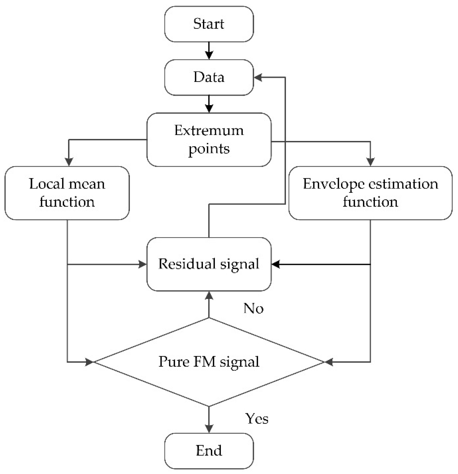
As explained above, the decomposition step of LMD is a multi-loop iterative process, first, a pure frequency modulation signal is obtained by iterating through the local extreme of the original signal, and then a PF component is obtained by further iteration, and so on, until all PFs are separated out. The decomposition flow chart of LMD is shown in Figure 4. FM signal in the figure represents the frequency modulation signal.

4.2. Selection of Characteristic PFs Based on Pearson Correlation Coefficient

In general, a series of PFs characterizing different feature scales can be obtained by LMD of the vibration signals. To quantify the correlation degree between PFs and the original signal, the Pearson correlation coefficient is introduced, as shown in Equation (12). The Pearson correlation coefficient is a value between −1 and 1, with the value tending to −1 or 1 when the correlation between the two variables strengthens and to 0 when the correlation between the two variables weakens. In general, the correlation coefficient less than or equal to 0.2 [58] implies that the two variables are not correlated; this principle is adopted in this paper. If the correlation coefficient between a PF component and the original data is less than or equal to 0.2, the PF component is discarded and the retained PFs are called the characteristic PFs. After the selection of Pearson correlation coefficients, the noise and the environmental vibration of the original signal were discarded and the components useful for damage identification were retained.
ρ X , Y = cov ( X , Y ) σ X σ Y
where X represents the original data and Y represents the PFs.

4.3. Time-Domain Feature Extraction

When the track structure is in the deformed state, the waveform of the vibration signal definitely changes [59]. The time-domain analysis method analyzes the system intuitively and accurately in the time domain and can be used to conduct structural damage identification studies by calculating the time-domain characteristic parameters of the vibration signal to reflect the relevant information of the vibration signal. It has been shown that the hierarchical function obtained by the adaptive decomposition method carries more damage information and is more sensitive to damage after decomposition [60]. Therefore, this paper employs the peak-to-peak acceleration, variance, root mean square, shape factor, crest factor, and skewness of the characteristic PFs [52] as time-domain feature indicators. Time-domain feature analysis is performed separately for the characteristic PFs and then the average value is taken as the feature vector. Table 1 lists the specific information of the time-domain features.
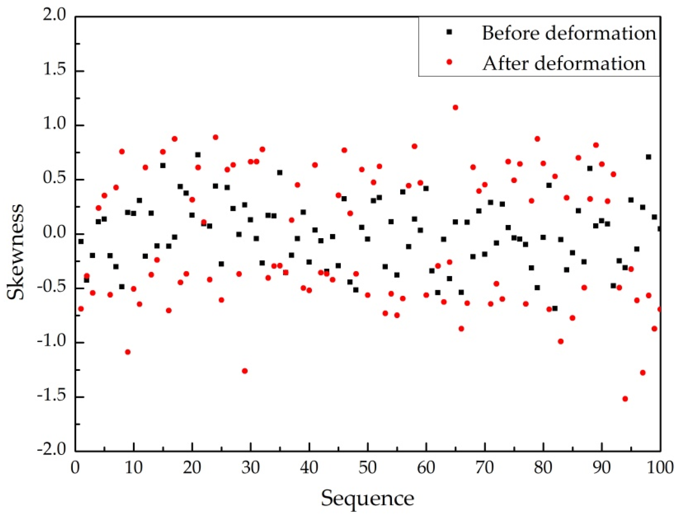
The amplitude of the vibration can only describe the instantaneous value of the vibration magnitude and does not include the time duration of vibration, and its root mean square value considering the time duration can characterize the magnitude of the vibration signal energy. The numerator in time-domain feature indicators of peak-to-peak acceleration, shape factor, and crest factor are the maximum value of vibration amplitude, highlighting the role of large amplitude. In addition, shape factor and crest factor can detect the presence of shocks in the vibration response signal. Variance can effectively characterize the extent to which a random variable deviates from its mean and, to a certain extent, can reflect the stability of the signal. Skewness can reflect the distribution characteristics of the vibration signal waveform. Due to the limitation of length, this paper only shows the scatter plot of the skewness of the track slab in normal and deformed states, and the results are shown in Figure 5. In this paper, 100 data were randomly selected from the sample pool of normal and deformed states, respectively, for comparative analysis. The black boxes and red dots in the figure represent the skewness in normal and deformed states, respectively. It can be clearly seen that when the track slab is in the deformation state, the vibration waveform asymmetry increases. In the range of coordinates both less or greater than 0, the skewness of the damage condition is greater than that in the normal state. This phenomenon indicates that the vibration waveform asymmetry increases when track slab deformation occurs and the skewness index increases. This is consistent with the existing literature research results [61].

4.4. Time-Frequency-Domain Feature Extraction

When damage occurs to the track structure, the vibration energy distribution of the structure will change, and, therefore, the energy of the characteristic PFs of the track structure will change simultaneously. A certain location of the track structure at which damage occurs can be considered the location with reduced frequency softening to absorb more vibration energy, which leads to an increase in the energy entropy of the vibration response. Therefore, the energy entropy of characteristic PFs can be selected as one of the damage identification features [59]. The energy entropy of characteristic PFs is calculated by the following steps:
  • Calculate the energy of the qth characteristic PF:
E q = j = 1 l | P F q j | 2
where l is the length of a characteristic PF.
2.
Calculate the total energy of these r efficient characteristic PFs:
E = q = 1 r E q
3.
Calculate the energy entropy of characteristic PFs:
H = - q = 1 r p q log ( p q )
where p q = E q E is the percentage of the energy of the qth characteristic PF relative to the total energy entropy, and q = 1 r p q = 1 .
To better understand the model formulation, the variables and parameters that appear in this section are classified and named. The results are shown in Table 2.
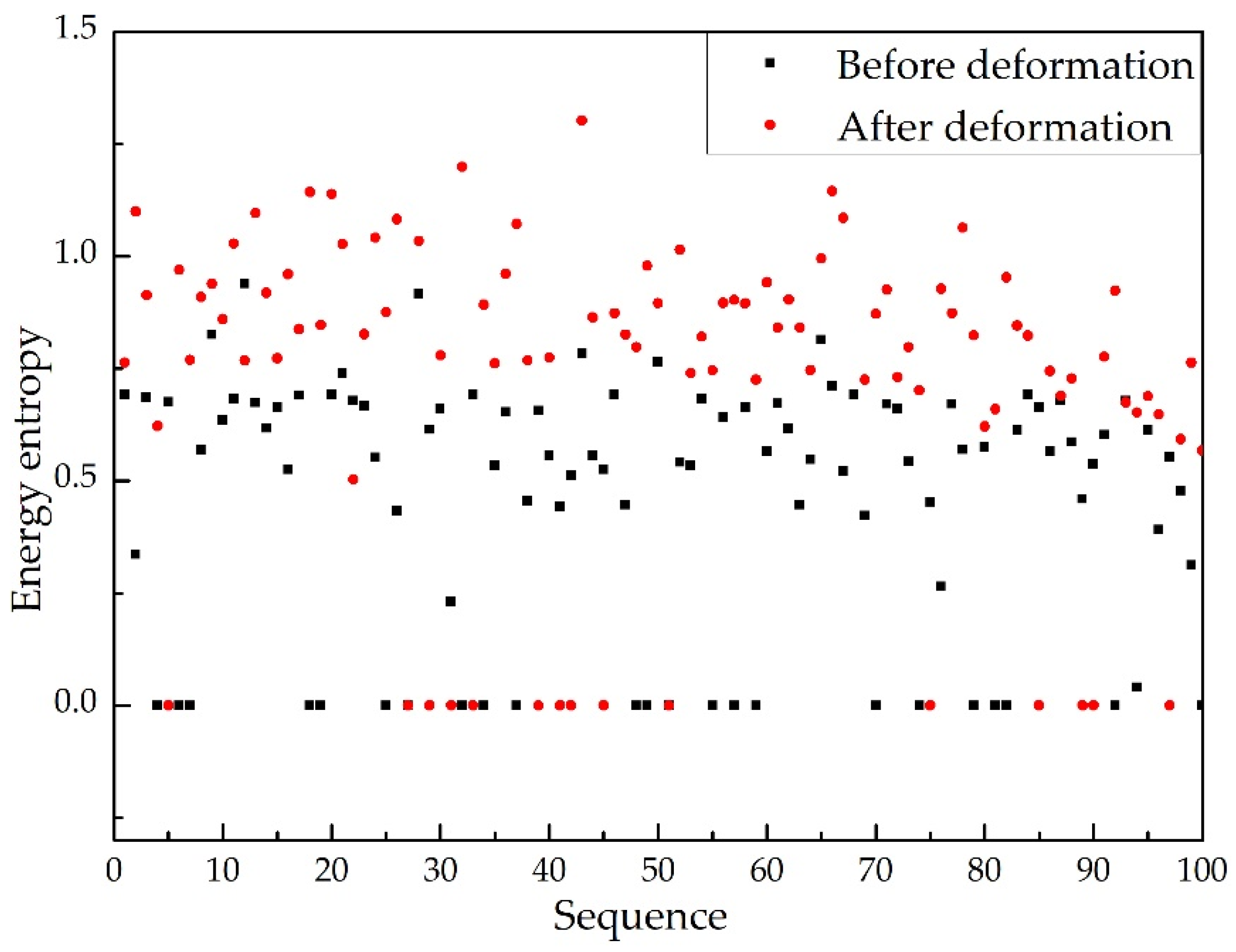
Figure 6 is a scatter plot of the energy entropy of the vibration response around track slab deformation. The black squares and red dots in the figure represent the energy entropy of the characteristic PFs in the normal and deformed state, respectively. Figure 6 indicates that the energy entropy of the characteristic PFs is larger in the deformed state, which is due to the damage of the track slab. When the track slab is in the deformation state, the structural stiffness decreases and the position needs to absorb more energy to achieve the equilibrium state; thus, the energy entropy increases. This is consistent with the existing literature results [62].
In this section, LMD is performed on the vibration data into several PFs, and the characteristic PFs are then selected with Pearson correlation coefficients. Six time-domain statistics and one time-frequency-domain feature are extracted from the characteristic PFs, which form a characteristic parameter vector matrix.

5. Establishment of Random-Forest Model

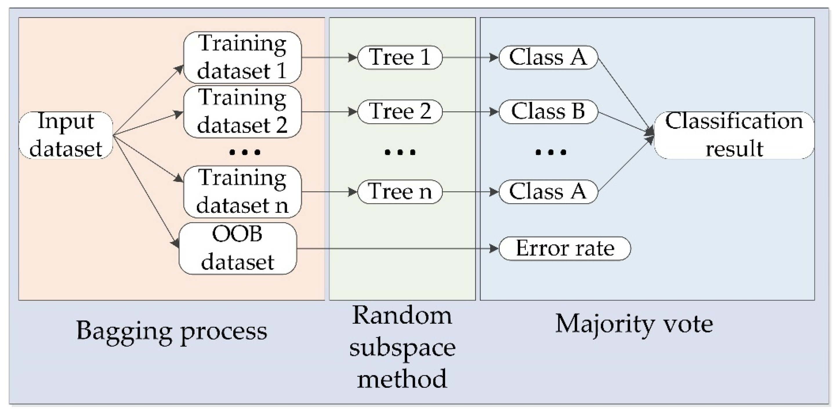
Random forest [63] is an ensemble machine learning algorithm with CART decision trees as the base classifier, where each decision tree is generated independently and completely split. It can solve both classification and regression problems by combining multiple independent decision trees based on voting or taking the average value; this approach tends to have higher accuracy and greater stability than using a single decision tree. Each decision tree is generated according to the following rules: (1) For a training set size of N, for each decision tree, N training samples that are put back are taken randomly from the training set as the training set. Approximately two-thirds of the observations are selected more than once, while the rest will not be chosen. The remaining one-third is called “out of bag” (OOB). (2) If the feature dimension of each sample is M, a subset of mtry features is randomly selected from M features (mtry << M), and mtry is called the split features. When the decision tree is split, the best of these mtry features is selected for splitting. Each tree grows to the greatest extent and without the pruning process. (3) To classify the samples of the testing set, the classification label is the majority vote decision of the decision trees. The introduction of random samples and random variables is crucial to the classification performance of the random-forest model. The former enables the model to have a more stable resistance to overfitting, and the latter enables it to have a higher accuracy rate than the decision tree method. The architecture of the random-forest model is shown in Figure 7. The working process is summarized as follows: random samples are input to each independent decision tree for classification, and each decision tree provides independent results. For the classification problem, the final decision is made by considering the majority of votes to determine the classification result.
The random-forest model classification performance is related to two factors [52]: the correlation of any two trees (the higher the correlation, the higher the error rate) and the classification ability of each tree (the stronger the classification ability, the lower the error rate). The classification ability of a tree and the correlation between two trees increases with the split features mtry. Therefore, the key problem is to determine the optimal split features mtry such that the classification ability and correlation are balanced, which is a parameter of the random-forest model. In addition, the more the number of decision trees, the better the randomization of the model, and thus the smaller the testing error of the model. Theoretically, the more the number of decision trees T, the better the randomization. With increasing number of decision trees, the test error variation decreases; hence, a reasonable number of trees can be determined. Hence, the split features mtry and the number of decision trees T are the two parameters of the random-forest model. The number of decision trees in the random-forest model can be determined by modifying the split features mtry and OOB error, while the error can be adjusted by changing the split features mtry and the number of decision trees T.

6. Results and Discussion

6.1. Random-Forest Model Results

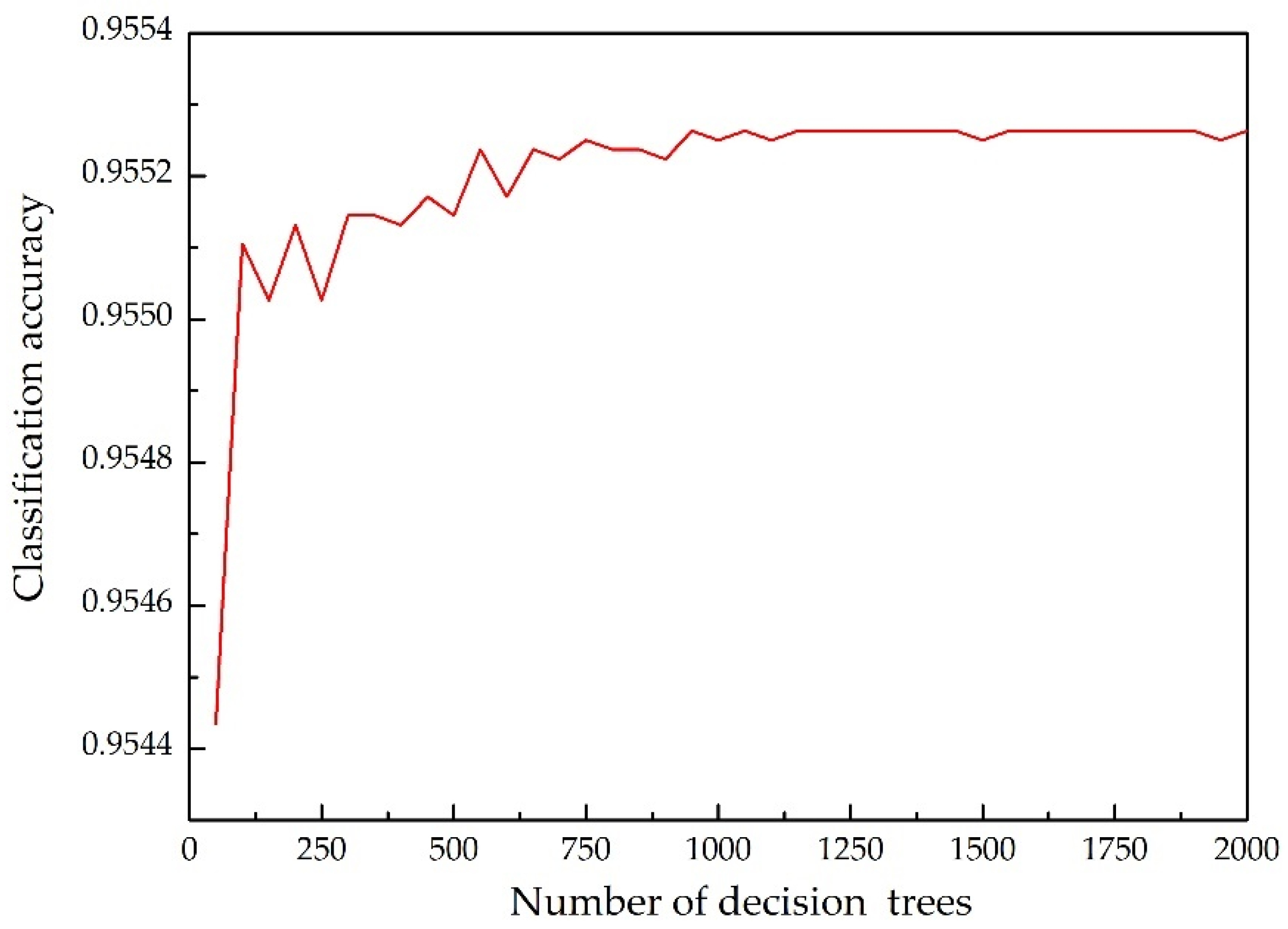
In this section, the results of the random-forest model and the model parameter optimization are presented. As mentioned in the previous section, fiber optic accelerometers are installed adjacent to the operating HSR to continuously acquire vibration data of the track slab in the normal and deformed states continuously. First, raw data are preprocessed with data interception, denoising, and segmentation. Then, the data are decomposed by LMD, and the characteristic PFs are selected on the basis of Pearson correlation coefficients. Finally, six time-domain feature parameters and one time-frequency-domain feature parameter are calculated of the selected characteristic PFs. Therefore, seven features can be extracted from the dataset to form the characteristic parameter vector matrix. For conducting evaluation analysis after the model development, the total dataset is divided into training and testing datasets. In this study, the dataset comprises 2534 samples, that is, 1875 and 659 samples for the normal and deformed states of track slab, respectively. Of the total data, 70% is used for the training set and the rest for the testing and validation of the results. During the development of the random-forest model, the number of decision trees T and the split features mtry are determined. In general, the split features mtry = (M) 1/2; in this paper, M = 7, so we let mtry = 3. The number of decision trees in random-forest model is determined according to the relationship between the number of decision trees and the classification accuracy, as shown in Figure 8. The classification accuracy tends to be stable when the number of decision trees reaches 1300. Given that the more decision trees, the better the randomization performance of the model, the number of decision trees in this paper is set to be 2000.
After the number of decision trees in the random-forest model is determined, the split features mtry need to be determined. When the classification accuracy reaches the maximum, the number of split features is considered to be optimal. Table 3 shows the effect of the number of split features mtry on the classification accuracy when the number of decision trees T is equal to 2000.
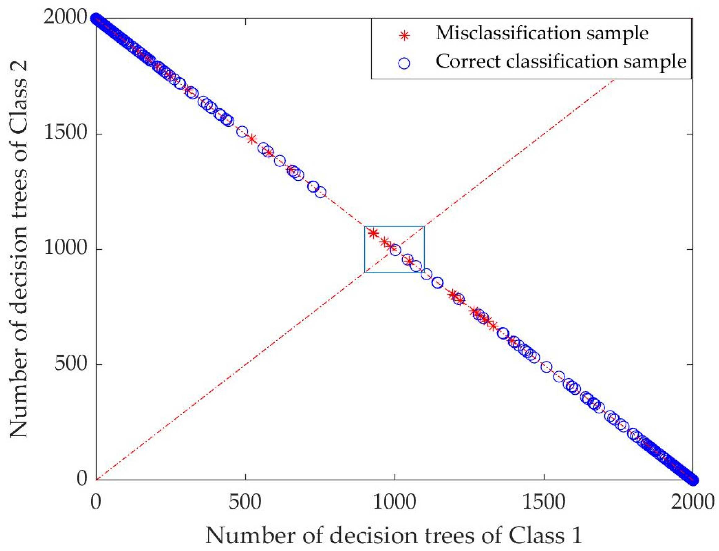
The best performance of the random-forest model to recognize Class 1 reaches 98.18% accuracy when mtry is set to 1. Similarly, the random-forest model using 3 split features (mtry = 3) can well identify Class 2 with 95.59% accuracy. Considering the average classifying accuracy, the random-forest models employing 3, 4, and 7 split features can achieve relatively higher accuracy (96.09%, 95.79%, and 94.58%) compared with other cases. It is also worth noting that more attention should be paid to the recognition accuracy of Class 2, because the deformed state may affect the safe operation of the HSR. From the model perspective, the split features mtry balances the strength of the trees as well as the correlation of the trees in the random-forest model. Therefore, in this paper, the split features mtry = 3 and the number of decision trees T = 2000 are used as the optimization parameters of the random-forest model. Figure 9 illustrates the results of random-forest classification using these optimized parameters (mtry = 3, T = 2000).
The points in Figure 9 represent the number of decision trees for both classifications, the horizontal coordinate represents the number of decision trees whose voting result is Class 1, and the vertical coordinate represents the number of decision trees whose voting result is Class 2. Since the total number of decision trees is 2000, all points are on the diagonal (x + y = 2000, x represents the number of decision trees whose voting result is Class 1, and y represents the number of decision trees whose voting result is Class 2). The red asterisks in the figure represent misclassified samples and the blue circles represent correctly classified samples. The samples in the blue boxes in Figure 9 represent close voting results and are prone to misclassification. Therefore, the closer the sample points are to the coordinates (2000, 0) and (0, 2000), the better is the performance of the model. It can be seen that, in the figure, most of the samples are concentrated at the two coordinates mentioned above, which indicates that the proposed random-forest model has a good classification performance. From a quantitative perspective, the total number of samples in the blue box is 7, accounting for 0.92% of the total testing set; this is a small percentage of the data, indicating that this random-forest model has a good classification effect.

6.2. Decision-Tree Model Results

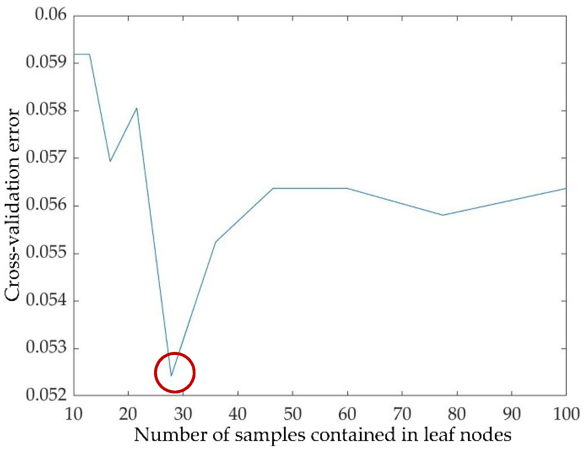
To verify the superiority of the proposed framework, we adopt a decision-tree model for a comparison study. The decision-tree model is a predictive model with an attribute structure that represents a mapping relationship between object attributes and object values [51]. A decision tree contains a root node and a number of internal nodes and leaf nodes. The root node contains the entire set of samples, the internal node represents a feature or attribute, and the leaf node represents a class. The path from the root node to each leaf node corresponds to a sequence of decision tests. Decision-tree learning essentially generalizes a set of classification rules from a training set to obtain a decision tree that is less contradictory to the dataset, while having good generalization ability [64]. In this paper, the ID3 algorithm and information gain principle are adopted to calculate and select the attribute with the greatest information gain as the classification attribute. In general, a number of attempts are needed to determine the sample number contained in leaf nodes to achieve good performance. Even a small sample number contained in leaf nodes will considerably affect the generalization ability of the decision-tree model. In this study, the cross-validation method is used to determine the sample number contained in leaf nodes to optimize the decision-tree model. Figure 10 shows the relationship between the number of samples contained in leaf nodes and the cross-validation error. The smaller the cross-validation error, the better is the generalization ability of the decision-tree model. As shown by the red circle in the figure, when the sample number contained in leaf nodes is 28, the cross-validation error is the smallest at 0.0523 and the decision-tree model generalization ability is the best. The decision-tree model is optimized for improved performance using the cross-validation method.
During decision-tree model learning, the node partitioning process will be repeated for classifying the training samples as accurately as possible. This sometimes results in overfitting because of too many branches in the decision-tree model. Therefore, the risk of overfitting can be reduced by actively removing some branches. In this study, the original decision-tree is pruned for comparison. The classification accuracy and cross-validation error of the original, optimized and pruned decision-trees are compared to determine the best performance of decision-tree model. Table 4 shows the classification accuracy and cross-validation error of the original, optimized, and pruned decision-tree.
As shown in Table 4, the cross-validation error reduced from 6.76% to 5.23% and the average classification accuracy increased from 91.49% to 93.06% by optimizing the original decision-tree; the cross-validation error reduced from 6.76% to 6.26% and the average classification accuracy increased from 91.49% to 92.51% by pruning the original decision-tree. Therefore, both optimizing and pruning of the original decision-tree can improve the generalization performance of the decision tree, with increased Class 1, Class 2, and average classification accuracy. In particular, the cross-validation error of the optimized decision-tree is smaller than that of the pruned decision-tree, indicating that optimization makes the decision-tree model generalize better than pruning. Therefore, the optimized decision-tree classification accuracy is higher than that of pruning, which is consistent with the above results. In summary, for the recognition of track slab deformation in this study, the original decision-tree needs to be optimized without pruning, and the classification accuracies of Class 1 and Class 2 are 94.96% and 91.15%, respectively, with an average classification accuracy of 93.06%. Comparison of the classification results shown in Table 3 indicates that the average classification accuracy of the random-forest model is higher than that of decision-tree model regardless of the value of split features. This confirms that the proposed random-forest model is better than the decision-tree model for the identification of track slab deformation.

7. Conclusions

In this paper, we proposed a method to analyze the health state of HSR using data-driven approaches based on on-site monitoring data. A novel random-forest-based strategy that combines LMD, time-domain feature extraction, and time-frequency-domain feature extraction for identification of track slabs deformation was proposed. The main conclusions are as follows.
  • A track-side vibration monitoring method based on fiber optic vibration sensing technology can effectively capture vibration signals that contain the information of train vibration, track slab deformation, noise, and environmental vibration.
  • The preprocessing methods of data interception, denoising, and data segmentation can effectively eliminate the effects of environmental vibration, noise, and time differences on the recognition effects. In addition, the time-domain and time-frequency-domain feature extraction methods based on LMD effectively extract the crucial information for detecting the deformation of track slabs.
  • The proposed intelligent recognition algorithm based on random-forest model can accurately identify the deformation of track slabs. The verification test results showed that the recognition accuracy reached 96.09%.
This paper provides not only a new method for operational HSR deformation monitoring but also an intelligent identification algorithm for track slab deformation identification. More importantly, the proposed method is applicable to the monitoring and identification of other structural defects. In the future, we will research the random-forest model on the deformation degree of track slabs.

Author Contributions

Conceptualization, G.G.; methodology, G.G.; software, G.G.; validation, G.G.; writing—original draft preparation, G.G.; writing—review and editing, G.G. and X.C.; project administration, B.D.; supervision, B.D. All authors have read and agreed to the published version of the manuscript.

Funding

This research was funded by National Natural Science Foundation of China (51822802, 51778033, U1811463, 71901011, and 51991395), National Key R&D Program of China (2018YFB2101003), The Science and Technology Major Project of Beijing (Z191100002519012) and Shenzhen Science and Technology Program (KQTD20180412181337494).

Institutional Review Board Statement

Not applicable.

Informed Consent Statement

Not applicable.

Acknowledgments

The authors thank Wentao Zhang at the Semiconductor Research Institute of Chinese Academy of Sciences for his provision of optical fiber sensing equipment. The authors would like to thank all the reviewers who participated in the review.

Conflicts of Interest

The authors declare no conflict of interest.

References

  1. Gao, L.; An, B.; Xin, T.; Wang, J.; Wang, P. Measurement, analysis, and model updating based on the modal parameters of high-speed railway ballastless track. Measurement 2020, 161, 107891. [Google Scholar] [CrossRef]
  2. Statistical Bulletin 2020 of China Railway. Available online: http://baijiahao.baidu.com/s?id=1691683529166535242 (accessed on 18 March 2021).
  3. Wang, P.; Xu, H.; Chen, R. Effect of cement asphalt mortar debonding on dynamic properties of CRTS II slab ballastless track. Adv. Mater. Sci. Eng. 2014, 2014, 1–8. [Google Scholar] [CrossRef] [Green Version]
  4. Li, Z.W.; Liu, X.Z.; He, Y.L. Identification of temperature-induced deformation for HSR Slab track using track geometry measurement data. Sensors 2019, 19, 5446. [Google Scholar] [CrossRef] [Green Version]
  5. Yang, M.H. Temperature warping deformation and modification of longitudinal slab-type ballastless track structure on bridge. China Railw. 2012, 04, 78–81. [Google Scholar]
  6. Li, Y.; Chen, J.J.; Wang, J.X.; Shi, X.F.; Chen, L. Analysis of damage of joints in CRTS II slab track under temperature and vehicle loads. KSCE J. C. Eng. 2020, 24, 1209–1218. [Google Scholar] [CrossRef]
  7. Gao, L.; Liu, Y.; Zhong, Y.L.; You, M.X.; Xin, T. Influence of damage of wide and narrow joints on mechanical performance of CRTS II slab-type ballastless track CWR. Railw. Eng. 2016, 5, 58–63. [Google Scholar]
  8. Xu, Y.D.; Yan, D.B.; Zhu, W.J.; Zhou, Y. Study on the mechanical performance and interface damage of CRTS II slab track with debonding repairment. Constr. Build. Mater. 2020, 257, 119600. [Google Scholar] [CrossRef]
  9. Shi, H.; Yu, Z.J.; Shi, H.M.; Zhu, L.Q. Recognition algorithm for the disengagement of cement asphalt mortar based on dynamic responses of vehicles. Proc. Inst. Mech. Eng. Part F J. Rail Rapid Transit 2018, 233, 270–282. [Google Scholar] [CrossRef]
  10. Yu, C.Y.; Xiang, J.; Mao, J.H.; Gong, K.; He, S.Y. Influence of slab arch imperfection of double-block ballastless track system on vibration response of high-speed train. J. Braz. Soc. Mech. Sci. Eng. 2018, 40, 109. [Google Scholar] [CrossRef]
  11. Ma, Z.R.; Gao, L.; Zhong, Y.L.; Ma, S.; An, B.L. Arching detection method of slab track in high-speed railway based on track geometry data. Appl. Sci. 2020, 10, 6799. [Google Scholar] [CrossRef]
  12. Cai, X.P.; Luo, B.C.; Zhong, Y.L.; Zhang, Y.R.; Hou, B.W. Arching mechanism of the slab joints in CRTS II slab track under high temperature conditions. Eng. Fail. Anal. 2019, 98, 95–108. [Google Scholar] [CrossRef]
  13. Zhao, L.; Zhou, L.Y.; Zhang, G.C.; Wei, T.Y.; Mahunon, A.D.; Jiang, L.Q.; Zhang, Y.Y. Experimental study of the temperature distribution in CRTS II ballastless tracks on a high-speed railway bridge. Appl. Sci. 2020, 10, 1980. [Google Scholar] [CrossRef] [Green Version]
  14. Zhu, S.Y.; Cai, C.B. Interface damage and its effect on vibrations of slab track under temperature and vehicle dynamic loads. Int.J. Nonlin. Mech. 2014, 58, 222–232. [Google Scholar] [CrossRef]
  15. Singh, M.; Singh, S.; Jaiswa, J.; Hernpshall, J. Autonomous rail track inspection using vision based system. In Proceedings of the IEEE International Conference on Computational Intelligence for Homeland Security & Personal Safety, Alexandria, VA, USA, 16–17 October 2006. [Google Scholar]
  16. Resendiz, E.; Hart, J.M.; Ahuja, N. Automated Visual Inspection of Railroad Tracks. IEEE T. Intell. Transp. 2013, 14, 751–760. [Google Scholar] [CrossRef] [Green Version]
  17. Yin, F. Research on detection method of gap caused by camber of CRTS II track slab. Railw. Eng. 2018, 58, 117–120. [Google Scholar]
  18. Ke, Y.T.; Cheng, C.C.; Lin, Y.C.; Ni, Y.Q.; Hsu, K.T.; Wai, T.T. Preliminary study on assessing delaminated cracks in cement asphalt mortar layer of high-speed rail track using traditional and normalized impact–echo methods. Sensors 2020, 20, 3022. [Google Scholar] [CrossRef]
  19. Xu, J.M.; Wang, P.; An, B.Y.; Ma, X.C.; Chen, R. Damage detection of ballastless railway tracks by the impact-echo method. Proc. Inst. Civ. Eng. Transp. 2018, 171, 106–114. [Google Scholar] [CrossRef]
  20. Pierre, A.B. Performance Evaluation of Impact Echo Method for Detection of Cavity Underneath a Concrete Slab Track Using Finite Element Method. Master’s Thesis, Pai Chai University, Daejeon, Korea, June 2019. [Google Scholar]
  21. Yang, Y.; Zhao, W.G. Curvelet transform-based identification of void diseases in ballastless track by ground penetrating radar. Struct. Control Health Monit. 2019, 26, e2322. [Google Scholar] [CrossRef]
  22. Liao, H.J.; Zhu, Q.N.; Jiu, Y.W.; Xie, Y.Y.; Sun, J.Y. Detection of ballastless track diseases in high-speed railway based on ground penetrating radar. J. Southwest Jiaotong Univ. 2016, 51, 8–13. [Google Scholar]
  23. Zhang, J.X.; Huang, W.Z.; Zhang, W.T.; Li, F.; Du, Y.L. Train-induced vibration monitoring of track slab under long-term temperature load using fiber-optic accelerometers. Sensors 2021, 21, 787. [Google Scholar] [CrossRef]
  24. Hussaini, S.K.K.; Indraratna, B.; Vinod, J.S. Application of optical-fiber Bragg grating sensors in monitoring the rail track deformations. Geotech. Test. J. 2015, 38, 387–396. [Google Scholar] [CrossRef] [Green Version]
  25. Chapeleau, X.; Sedran, T.; Cottineau, L.M.; Cailliau, J.; Taillade, F.; Gueguen, I.; Henault, J.M. Study of ballastless track structure monitoring by distributed optical fiber sensors on a real-scale mockup in laboratory. Eng. Struct. 2013, 56, 1751–1757. [Google Scholar] [CrossRef]
  26. Milne, D.; Masoudi, A.; Ferro, E.; Waston, G.; Louis, L.P. An analysis of railway track behaviour based on distributed optical fibre acoustic sensing. Mech. Syst. Signal Pr. 2020, 142, 106769. [Google Scholar] [CrossRef]
  27. Wang, Z.C.; Zhao, Z.G.; Chai, X.S.; Jin, M.; Feng, Y.J.; Ling, L.P.; Liu, Y.F. Research on monitoring technology of track slab upwarp based on distributed optical fiber sensing. Railw. Eng. 2020, 60, 42–45. [Google Scholar]
  28. Gao, W.H. Study on Analytical Method of Track Geometrical Irregularities for High-Speed Railway. Master’s Thesis, Beijing Jiaotong University, Beijing, China, 2020. [Google Scholar]
  29. Duan, Z.Q.; Meng, E.L.; Wang, L.M.; Li, H. Fault diagnosis for wind turbine transmission systems via demodulation analysis based on EEMD and energy separation. Noise. Vib. Control 2018, 38, 161–166. [Google Scholar]
  30. Huang, N.E.; Shen, Z.; Long, S.R.; Wu, M.L.C.; Shih, H.H.; Zheng, Q.N.; Yen, N.C.; Tung, C.C.; Liu, H.H. The empirical mode decomposition and the Hilbert spectrum for nonlinear and non-stationary time series analysis. P Math. Phy. Eng. Sci. 1998, 454, 903–995. [Google Scholar] [CrossRef]
  31. He, Y.F. Research on the Rail Defect Detection and Identification of the Urban Rail Transit. Master’s Thesis, Beijing Jiaotong Unviersity, Beijing, China, 2016. [Google Scholar]
  32. Ning, J. Study on the Time-Frequency Analysis by EMD and Cohen’s Kernel and Application in Track. Ph.D. Thesis, Southwest Jiaotong University, Sichuan, China, 2011. [Google Scholar]
  33. Chen, X.M. Time-Frequency Analysis and Prediction Study on Track Irregularities. Ph.D. Thesis, Institute of Railway Science, Beijing, China, 2006. [Google Scholar]
  34. Chen, T.T.; Zhao, W.G.; Li, R.Z.; Yang, Y.; Tian, X.S. Study on identification of CA mortar layer void based on convolution neural network. Railw. Stand. Des. 2021, 65, 1–8. [Google Scholar]
  35. Smith, J.S. The local mean decomposition and its application to EEG perception data. J. R. Soc. Interface 2005, 2, 443–454. [Google Scholar] [CrossRef]
  36. Gu, Z.Q.; Lin, Y.D. Fault diagnosis of rolling bearing based on improved LMD and comprehensive characteristic index. J. Hefei Univ. Tech. Nat. Sci. 2021, 44, 145–150. [Google Scholar]
  37. Zhang, Y.L.; Zhang, P.J.; Fang, Y.H.; Dong, X.Y. Research on signal feature extraction method of LMD-KICA rolling bearing. Mach. Des. Manuf. 2021, 02, 15–18. [Google Scholar]
  38. Li, X.; Ma, J.; Wang, X.D.; Wu, J.D.; Li, Z.R. An improved local mean decomposition method based on improved composite interpolation envelope and its application in bearing fault feature extraction. ISA Trans. 2020, 97, 365–383. [Google Scholar] [CrossRef]
  39. Kocbek, S.; Gabrys, B. Automated machine learning techniques in prognostics of railway track defects. In Proceedings of the International Conference on Data Mining Workshops (ICDMW), Beijing, China, 8–11 November 2019. [Google Scholar]
  40. Li, D.; Wang, Y.; Yan, W.J.; Ren, W.X. Acoustic emission wave classification for rail crack monitoring based on synchrosqueezed wavelet transform and multi-branch convolutional neural network. Struct. Health Monit. 2020, 2, 147592172092279. [Google Scholar] [CrossRef]
  41. Zhan, Y.; Dai, X.X.; Yang, E.H.; Wang, K.C.P. Convolutional neural network for detecting railway fastener defects using a developed 3D laser system. Int. J. Rail Transp. 2020, 1–21. [Google Scholar] [CrossRef]
  42. Yao, D.C.; Sun, Q.; Yang, J.W.; Liu, H.C.; Zhang, J. Railway fastener fault diagnosis based on generative adversarial network and residual network model. Shock. Vib. 2020, 2020, 8823050. [Google Scholar] [CrossRef]
  43. Cui, H.; Li, J.; Hu, Q.W.; Mao, Q.Z. Real-time inspection system for ballast railway fasteners based on point cloud deep learning. IEEE Access 2020, 8, 61604–61614. [Google Scholar] [CrossRef]
  44. Wei, X.K.; Yang, Z.M.; Liu, Y.X.; Wei, D.H.; Jia, L.M.; Li, Y.J. Railway track fastener defect detection based on image processing and deep learning techniques: A comparative study. Eng. Appl. Artif. Intel. 2019, 80, 66–81. [Google Scholar] [CrossRef]
  45. Ferreno, D.; Sainz-Aja, J.A.; Carrascal, I.A.; Guartas, M.; Pombo, J.; Casado, J.A.; Diego, S. Prediction of mechanical properties of rail pads under in-service conditions through machine learning algorithms. Adv. Eng. Softw. 2021, 151, 102927. [Google Scholar] [CrossRef]
  46. Zhuang, Z.; Zhang, G.H.; Dong, W.; Sun, X.Y.; Wang, C.J. Intelligent fault detection of high-speed railway turnout based on hybrid deep learning. In Proceedings of the 31st Australasian Joint Conference on Artificial Intelligence, Wellington, New Zealand, 11–14 December 2018. [Google Scholar]
  47. Li, W.J.; Shen, Z.H.; Li, P.G. Crack detection of track plate based on YOLO. In Proceedings of the 12th International Symposium on Computational Intelligence and Design (ISCID), Hangzhou, China, 14–15 December 2019. [Google Scholar]
  48. Wang, W.; Hu, W.; Wang, W.; Xu, X.; Wang, M.; Shi, Y.; Qiu, S.; Tutumluer, E. Automated crack severity level detection and classification for ballastless track slab using deep convolutional neural network. Autom. Constr. 2021, 124, 103484. [Google Scholar] [CrossRef]
  49. Hu, Q.; Xu, W.; Gao, F.; Zhu, H.P. Damage identification of CA mortar layer of CRTS Ⅰ slab track based on BP neural network. J. Civ. Eng. Manag. 2018, 35, 90–96. [Google Scholar]
  50. Guo, G.R.; Cui, X.H.; Du, B.W. Monitoring technology for deformation of key sections of CRTS Ⅱ slab ballastless track foundation. China Railw. 2019, 11, 60–66. [Google Scholar]
  51. Zhou, Z.H. Machine Learning, 1st ed; Tsinghua University Press: Beijing, China, 2016; pp. 101–102. [Google Scholar]
  52. Zhang, L.H.; Ni, Y.Q.; Lai, S.; Wang, S.G. A novel machine learning technique for online health monitoring of high-speed trains. In Proceedings of the 2nd International Workshop on Structural Health Monitoring for Railway System, Qingdao, China, 17–19 October 2018. [Google Scholar]
  53. Chen, X.Y. Research and Application of Intrusion Detection Technology Based on Features Analysis and Support Vector Machines. Master’s Thesis, Beijing University of Posts and Telecommunications, Beijing, China, 2015. [Google Scholar]
  54. Meng, D.M. Study on the Structural Damage Identification Based on the Free Response Signal and Neural Network. Master’s Thesis, Qingdao Technological University, Qingdao, China, 2012. [Google Scholar]
  55. Breiman, L. Bagging predictors. Mach. Learn. 1996, 24, 123–140. [Google Scholar] [CrossRef] [Green Version]
  56. Jiang, D.S.; Zhang, W.T.; Li, F. All-metal optical fiber accelerometer with low transverse sensitivity for seismic monitoring. IEEE Sens. J. 2013, 13, 4556–4560. [Google Scholar] [CrossRef]
  57. Cheng, J.S.; Zhang, K.; Yang, Y.; Yu, D.J. Comparison between the methods of local mean decomposition and empirical mode decomposition. J. Vib. Shock 2009, 28, 13–17. [Google Scholar]
  58. Buda, A.; Jarynowski, A. Life Time of Correlations and its Applications; Wydawnictwo Niezalezne: Wroclaw, Poland, 2010; pp. 5–21. [Google Scholar]
  59. Wang, Y.M. Study on the Structural Damage Identification Based on the Response and PSO-SVM. Master’s Thesis, Qingdao University of Technology, Qingdao, China, 2019. [Google Scholar]
  60. Yuan, C.Q.; Zhao, D.; Yu, Y.H. Identifying the damage degree of structure based on empirical mode decomposition and parameters in time domain amplitude. Nondestruct. Test. 2008, 30, 84–86. [Google Scholar]
  61. Wu, S.S. Research on Void Detection Method of CRTS Ⅱ Slab Track Based on Transient Impulse Response. Master’s Thesis, Shijiazhuang Tiedao University, Shijiazhuang, China, 2018. [Google Scholar]
  62. Zhou, T.L. Research on Structural Damage Identification Method Based on CEEMD. Master’s Thesis, Changsha University of Technology, Changsha, China, 2016. [Google Scholar]
  63. Breiman, L. Random forests. Mach. Learn. 2001, 45, 5–32. [Google Scholar] [CrossRef] [Green Version]
  64. Koga, S.S.; Zhou, X.L.; Dickson, D.W. Machine learning-based decision tree classifier for the diagnosis of progressive supranuclear palsy and corticobasal degeneration. Neuropathol. Appl. Neurobiol. 2021, 00, 1–11. [Google Scholar]
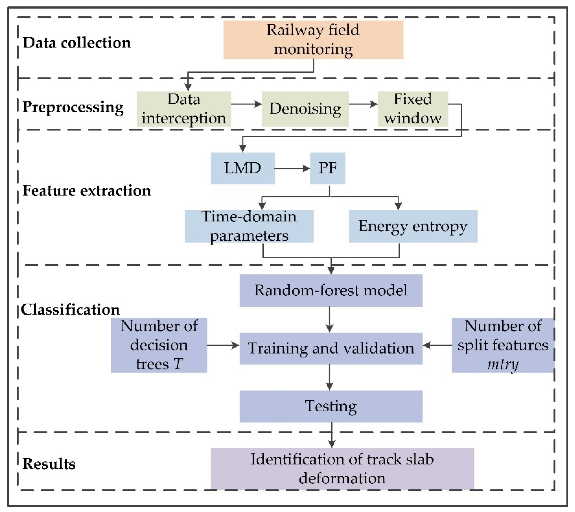
Figure 1. Flowchart of the deformation identification of a track slab.
Applsci 11 04756 g001
Figure 2. Field track-side monitoring system.
Applsci 11 04756 g002
Figure 3. Preprocessing process.
Applsci 11 04756 g003
Figure 4. Flow chart of LMD.
Applsci 11 04756 g004
Figure 5. Scatter plot of the skewness of the vibration response.
Applsci 11 04756 g005
Figure 6. Scatter plot of the energy entropy of the vibration response.
Applsci 11 04756 g006
Figure 7. Architecture of a random-forest classification model.
Applsci 11 04756 g007
Figure 8. Relationship between the number of decision trees and classification accuracy.
Applsci 11 04756 g008
Figure 9. Results of random-forest classification.
Applsci 11 04756 g009
Figure 10. Relationship between the number of samples contained in leaf nodes and the cross-validation error.
Applsci 11 04756 g010
Table 1. Summary of time domain features.
NameExpressionDescription
Peak-to-Peak V P P = max ( P F q ) min ( P F q ) The difference between the maximum and minimum values.
Variance s 2 = 1 r q = 1 r ( P F q P F ¯ ) 2 The average of the sum of squares of the difference between the data and the mean value.
Root mean square P F r m s = 1 r q = 1 r ( P F q ) 2 Indicates the magnitude of the energy of the vibration signal.
Shape factor f = P F r m s / 1 r q = 1 r | P F q | Refers to a value that is affected by the shape of waveforms.
Crest factor C = max ( P F q ) / P F r m s Detects the existence of shocks.
Skewness S k = 1 / r q = 1 r ( P F q P F ¯ ) 3 ( 1 / r q = 1 r ( P F q P F ¯ ) 2 ) 3 Measures the skewness of the data distribution
(Note: PFq represents the qth characteristic PF, P F ¯ represents the mean value of characteristic PFs, and r represents the number of characteristic PFs.)
Table 2. Nomenclature table of the model variables and parameters.
CategorySymbolName
variablesxVibration signal
tTime
NLocal extremum point
iLocal extremum point variable
mAverage of local extremum point
aLocal amplitude
hIntermediate process variable
sPure frequency modulation signal
PFProduct function
nnPure frequency modulation signal iteration count variable
kkMonotonic signal iteration count variable
uResidual signal
qNumber of characteristic product function variable
jLength of characteristic product function variable
ETotal energy
pNormalized energy
HEnergy entropy
parametersnPure frequency modulation signal iteration count
kMonotonic signal iteration count
rNumber of characteristic product function
lLength of characteristic product function
Table 3. Classification accuracy (%) with different number of split features.
Categorymtry = 1234567
Class 198.1896.6396.5897.8397.5096.5897.28
Class 291.5192.8995.5993.7591.4690.6991.87
Average94.8594.7696.0995.7994.4893.6494.58
(Note: Class 1 stands for the normal state of the track slab and Class 2 for the deformed state of the track slab).
Table 4. Classification accuracy (%) and cross-validation error (%).
CategoryOriginal
Decision-Tree
Optimized
Decision-Tree
Pruned
Decision-Tree
Class 193.6594.9694.05
Class 289.3291.1590.96
Average91.4993.0692.51
Error6.765.236.26
(Note: Error stands for the cross-validation error).
Publisher’s Note: MDPI stays neutral with regard to jurisdictional claims in published maps and institutional affiliations.