Solid-State Lithium Battery Cycle Life Prediction Using Machine Learning

Abstract

Battery lifetime prediction is a promising direction for the development of next-generation smart energy storage systems. However, complicated degradation mechanisms, different assembly processes, and various operation conditions of the batteries bring tremendous challenges to battery life prediction. In this work, charge/discharge data of 12 solid-state lithium polymer batteries were collected with cycle lives ranging from 71 to 213 cycles. The remaining useful life of these batteries was predicted by using a machine learning algorithm, called symbolic regression. After populations of breed, mutation, and evolution training, the test accuracy of the quantitative prediction of cycle life reached 87.9%. This study shows the great prospect of a data-driven machine learning algorithm in the prediction of solid-state battery lifetimes, and it provides a new approach for the batch classification, echelon utilization, and recycling of batteries.

1. Introduction

Lithium-ion batteries gradually becoming favored by the market because of their excellent performance and decreasing cost [1,2,3,4]. The demand for higher energy density and the concerns for safety issues of energy storage devices have also lead to the development of solid-state lithium batteries. First, solid-state batteries mitigate the safety risks by replacing the flammable organic liquid electrolytes with thermostable solid electrolytes. Second, solid electrolytes with a wider electrochemical window could enable the application of lithium metal anodes and certain cathodes with higher voltage capabilities and larger specific capacities [5,6]. However, the time-consuming electrochemical cycle life tests, which usually take months or years to determine the performance of concrete materials or systems, largely hinder the improvement of research efficiency for lithium batteries. Besides, cycle life is critical for the balanced design of cell packs and utilization of battery echelon [7]. The large-scale battery packs used in electric vehicles and energy storage power stations need multiple cells in series and parallel connection. The differences in cycle life of the paired batteries should be controlled in a narrow range or they will make battery balance difficult and will seriously affect the overall pack service life. Echelon utilization is even more dependent on the remaining useful life (RUL) of batteries to determine the price and application scenarios. Hence, the quick and precise estimation of useful battery life using early electrochemical test data will bring novel opportunities for battery research and application. In fact, RUL has been an increasingly more significant parameter in battery management systems, and it could provide predictive maintenance data for end users. The exploration for lithium battery modeling and degradation mechanisms has also become a research focus in energy storage fields [8,9,10].

Recently, advances in computational power, optimized algorithms, and data generation have enabled the wider application of machine-learning approaches in various projects, including battery degradation prediction [11,12,13,14,15,16,17,18,19]. For instance, Attia et al. established a closed-loop optimization system using elastic network regression and Bayesian optimization to predict the battery life and improve fast charging policies, and they compressed the original experimental period of over 500 days to 16 days [20]. Dai et al. also concentrated on the charging voltage curve of batteries to generate highly cycle life-correlated features. Interestingly, the influence of features on the state of health (SOH) is written into the loss function as a penalty factor, and the prior knowledge is thus embedded into the neural network to reduce the scope of parameter exploration and improve the optimization efficiency. Finally, the maximum prediction error of the SOH is less than 1.7% [21]. Liu et al. proposed a battery SOH assessment method based on different degradation features extracted from the voltage, electric current, and critical time during operation. These degradation features were fused and trained by the support vector regression mapping model that linked the feature space to the SOH space. The correlation between the degradation feature and the battery testing capacity was higher than 0.7, and the mean error of health estimation was less than 0.05 [22]. Zhou et al. constructed a temporal convolution network (TCN) using the dilation convolution technique, and they accurately captured the local regeneration of capacity with battery capacity sequence as the input. Then, empirical mode decomposition (EMD) was introduced to process the cycle data, which eliminated the error caused by local regeneration, and improved the RMSE accuracy of RUL prediction by 5% [23]. In addition to charge/discharge curves, other electrochemical test data have also been used to explore battery service performance. Zhang et al. used Gaussian process regression to deal with the electrochemical impedance spectroscopy of commercial lithium-ion batteries, and they successfully predicted the capacity and remaining cycle life of these batteries. By calculating the importance weight corresponding to different frequencies of the impedance spectrum, the interfacial impedance evolution represented by the low-frequency region was detected to be the focal points affecting battery capacity and degradation patterns [24]. Although the RUL prediction of liquid lithium-ion batteries has achieved a high accuracy, the RUL of solid lithium batteries is rarely reported due to the different degradation mechanisms, challenging performance variability, complicated interfacial reactions, and the lack of open-source test datasets [25]. In the following paragraph, some recent studies are reviewed to introduce the different degradation mechanisms between liquid and solid-state lithium batteries.

Many physical and chemical battery models have been proposed for diverse degradation mechanisms such as the growth of the solid electrolyte interphase, the fracture of lithium dendrites, active material loss, and interfacial polarization, which are listed in Figure 1 [26,27,28,29,30]. In general, the causes of battery degradation can be divided into two categories, capacity fading and impedance increases. Both have some related measurable physical quantities, while impedance information is more expensive to test and difficult to analyze. For commercial lithium-ion batteries, impedance does not change too much, because the liquid electrolyte wets the gaps inside electrode particles, as well as the gaps between electrodes and electrolytes [31]. In contrast, impedance increases take up a major degradation factor for solid-state batteries [6]. Delicate point contact is expected for solid-solid interfaces in solid-state batteries. These solid electrolyte/electrode interfaces significantly govern the electrochemical properties and cycle lifetime, as unwanted reaction products at the interface cannot dissolve and diffuse in the solid electrolyte [32,33]. Hence, it is necessary to employ both features to capture the electrochemical impedance evolution during degradation and to capture the capacity fading during cycling.

In this work, we chose symbolic regression (SR) as the prediction method considering the lack of a mature quantitative mapping formula between battery features and cycle life, as well as the strong nonlinear fitting ability of symbolic regression. The results showed that symbolic regression can accurately predict the RUL using the features derived from the voltage–time curves. To the best of our knowledge, the largest open-source solid-state lithium polymer battery charging and discharging dataset (LFP/Li or NCM/Li) was generated and made publicly available. After the extraction of features and parameter optimization, our models reached an 88% test accuracy for the quantitative prediction of the remaining cycle life. This work highlights the potential of data-driven methods to estimate the evolution of complex material systems, and it lays the foundation for the commercial application of solid-state lithium batteries in the future.

2. Materials and Methods

This section describes the generation of our battery cycle data and the methods we used for battery lifetime prediction. The features extracted from batteries are available at Zenodo (http://doi.org/10.5281/zenodo.4743315, accessed on 16 April 2021).

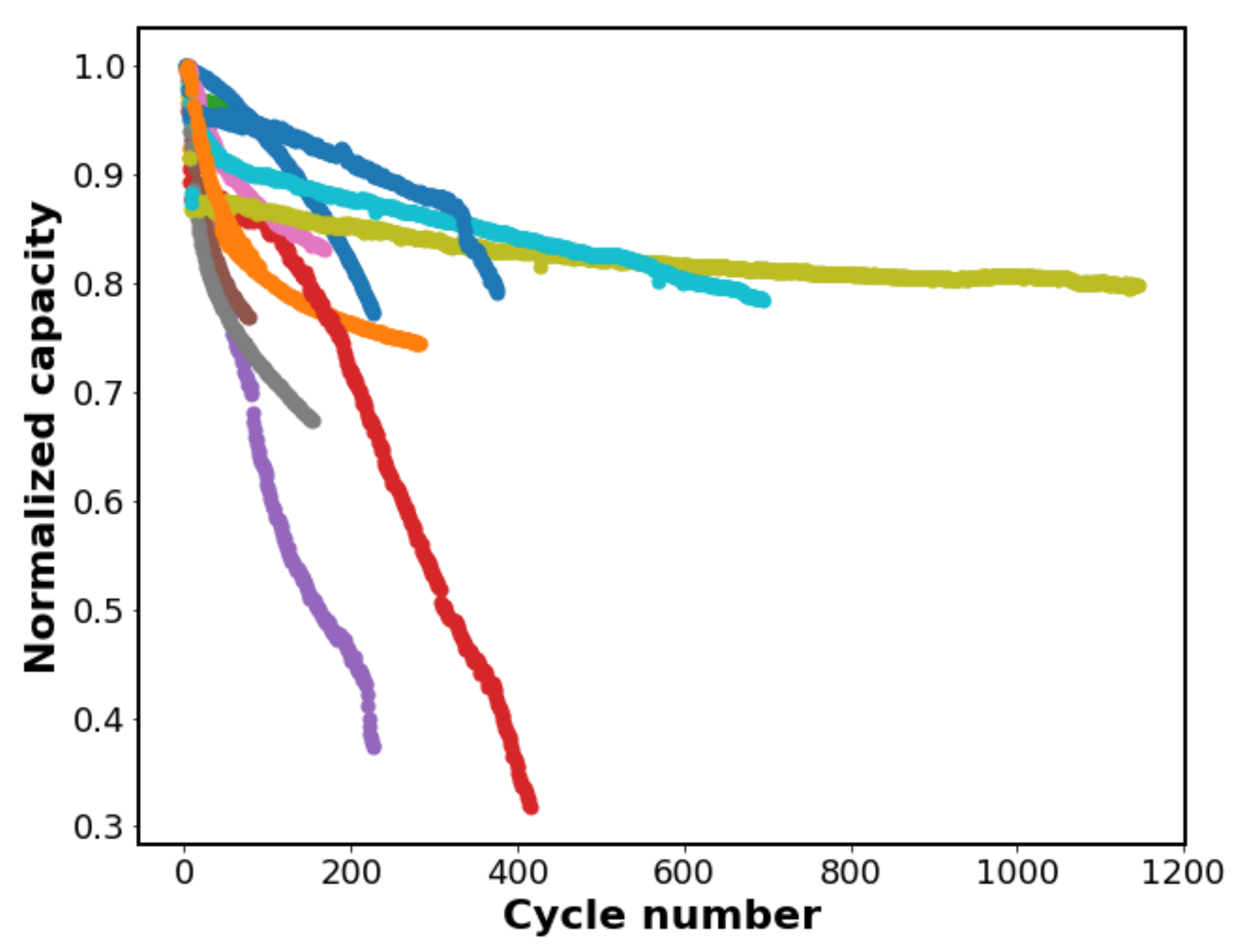
2.1. Battery Cycle Data Generation: Dataset Description

The dataset used in this work was composed of charge/discharge tests from 12 solid-state lithium polymer batteries. The cathode materials of 9 batteries were composed of lithium iron phosphate (LFP). The cut-off voltage range of the charge/discharge test was 2.0~3.65 V. The assembled LFP batteries were first charged with a constant current of 0.1 C, and the cutoff voltage was 3.65 V. When the voltage reached 3.65 V, they would charge at constant voltage with a cutoff current of 0.05 C. Then, they would discharge with a constant current of 0.1 C and a cutoff voltage of 2.0 V. The cycle tests were repeated until the battery capacity decayed to 80% of the nominal capacity. The cathode materials of the other 3 batteries were lithium nickel cobalt manganese oxide (NCM). The assembled NCM batteries were cycled in the same way as the LFP batteries were, while the cut-off voltage range was 3.0~4.2 V. The cross-linked nanocomposite polymer electrolytes (CNPEs) based on polyethylene oxide were prepared as described in our previous work from reference [34]. The LFP or NMC cathode was made of active materials with acetylene black and PVDF in the weight ratio of 8:1:1. Then, the CNPE films were sandwiched between the lithium anode and cathode film. All of the assembly processes were conducted under an argon environment in a glove box. These batteries were packaged in pouch cells and cycled in constant current using LAND Electronics with the temperature controlled at 25 °C. The tests were finished when the discharge capacity of the battery decreased to 80% of the initial discharge capacity. Due to the high-dimensional test data forms and intricate degradation mechanism of solid lithium batteries, we employed a data-driven approach using a series of descriptors extracted from the full voltage curves of each cycle. The specific feature selection and algorithm design are discussed in the next section.

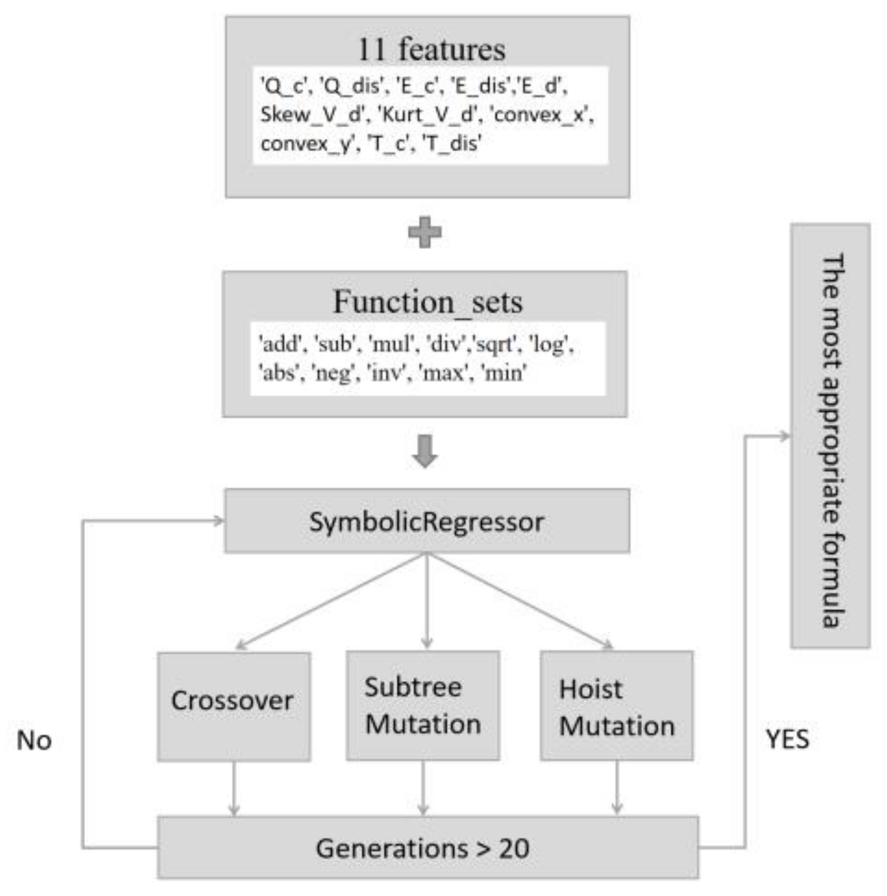
2.2. Feature Selection

Considering the lack of cycle-by-cycle impedance spectroscopy in our dataset and the impracticality and expensive cost of real-time impedance testing, we captured the impedance evolution from the voltage–time curve. Luckily, the voltage–time curve did reflect the battery aging information caused by impedance increases, and similar approaches have been proved efficient in previous work [35]. Due to the existence of internal impedance, the electrode potential deviated from the equilibrium potential when the current passed through the electrode. This phenomenon is called polarization, which produces overpotential, as shown in Figure 2. The result of polarization is that the terminal voltage of a battery is lower than the equilibrium potential when the battery is discharging and higher than the equilibrium potential when the battery is charging. Therefore, the working voltage curve of the battery becomes the superposition of polarization information inside the battery. For example, Koga et al. proved the efficiency of quasi-polarization, defined as half of the difference in the averaged value between the charge and discharge voltage curve. Quasi-polarization monotonically increases with cycle numbers and roughly estimates the evolution of polarization.

We also established a measure of polarization degree, which is the kurtosis of the charge/discharge voltage difference sequence (gray area), as shown in Figure 3a. Kurtosis is a common mathematical feature, which can be used to measure the steepness of the probability distribution of random variables. Its calculation formula is shown in Equation (4). The larger the kurtosis value, the more concentrated the probability distribution. The smaller the kurtosis value, the more uniform the probability distribution. As the overpotential caused by polarization concentrates at the beginning and end of the charge/discharge process in the early battery cycles, and then gradually fills the whole charge/discharge process, we proposed that the kurtosis value would decrease with the cycle numbers. As shown in Figure 3b, taking 6# battery as an example, its kurtosis value did monotonously decrease with the cycle numbers, which proves the correctness of our assumption. A correlation coefficient (ρ) was introduced to examine the correlation between features and the RUL [36]:

$$\rho =Cor\left(X_{feature},RUL\right)=\frac{cov\left(X_{feature},RUL\right)}{\sqrt{Var\left(X_{feature}\right)Var\left(RUL\right)}}$$

(1)

where X_feature denotes one of features we extracted from our dataset, ‘Cov’ stands for the covariance between variables, ‘Var’ represents the variance in the data, and RUL represents the cycle numbers of the remaining useful life [37]. The RUL for the ith cycle is calculated by

$$RU{L}_i=n+1-i$$

(2)

where n is the total number of battery charge and discharge cycles, and i is the ith charge and discharge cycle we chose to study. Equation (1) means the present cycle is also included in the remaining useful cycles.

Based on the above discussion of degradation mechanisms and analysis of charge/discharge curves, 30 features were selected for the RUL prediction (Supplementary Table S1). Some features represent the fading of capacity. The other features represent the increase in internal resistance. Furthermore, as shown in Figure 4, by sorting their coefficients of association between feature value and the RUL, 11 important features were retained, and they are described in detail below:

Feature 1–2: Charge/discharge time. Time of constant current charge/discharge progress. The duration indicates the capacity by which the battery can be charged. Hence, this phenomenon can reflect the battery degradation process.

Feature 3–4: Charge/discharge capacity. The total capacity of constant current charge/discharge progress.

Feature 5–6: the integral value of charge/discharge capacity–voltage curves: capacity–voltage curves are drawn with charge/discharge capacity as the x-coordinate and the output voltage as the y-coordinate. The integral value can be used as a measure of the energy, containing the heating energy consumed by the polarization internal resistance.

Feature 7–8: Turning point coordinates of capacity–voltage curve. Turning points are defined as the positions where the slope of the capacity–voltage curves dramatically change.

Feature 9–10: The kurtosis and skewness of difference between the charge and discharge voltage curve. Skewness, also known as the third-order central moment, can be used to measure the asymmetry of the probability distribution of random variables [38]. The formulation is:

$$S=\frac{1}{n}{{\displaystyle \sum }}_{i=1}^n\left[{\left(\frac{X_i-\mu }{\sigma }\right)}^3\right]$$

(3)

where S represents the skewness, n is the number of samples, X_i is the value of the ith sample (here, it is the voltage difference), and μ and σ are the mean and variance of the voltage difference sequence, respectively.

Kurtosis, also called fourth-order central moment, can be used to measure the steepness of the probability distribution of random variables [38]. The formulation is:

$$K=\frac{1}{n}{{\displaystyle \sum }}_{i=1}^n\left[{\left(\frac{X_i-\mu }{\sigma }\right)}^4\right]$$

(4)

where K represents the kurtosis, and n, X_i, μ, and σ are the same as those in Equation (3). Here, we have subtracted the value by 3 so that the kurtosis of the normal distribution is zero, which also explains the negative kurtosis values in Figure 3b.

Feature 11: Energy dissipation. The difference value of feature 5 and feature 6.

2.3. Algorithm Selection

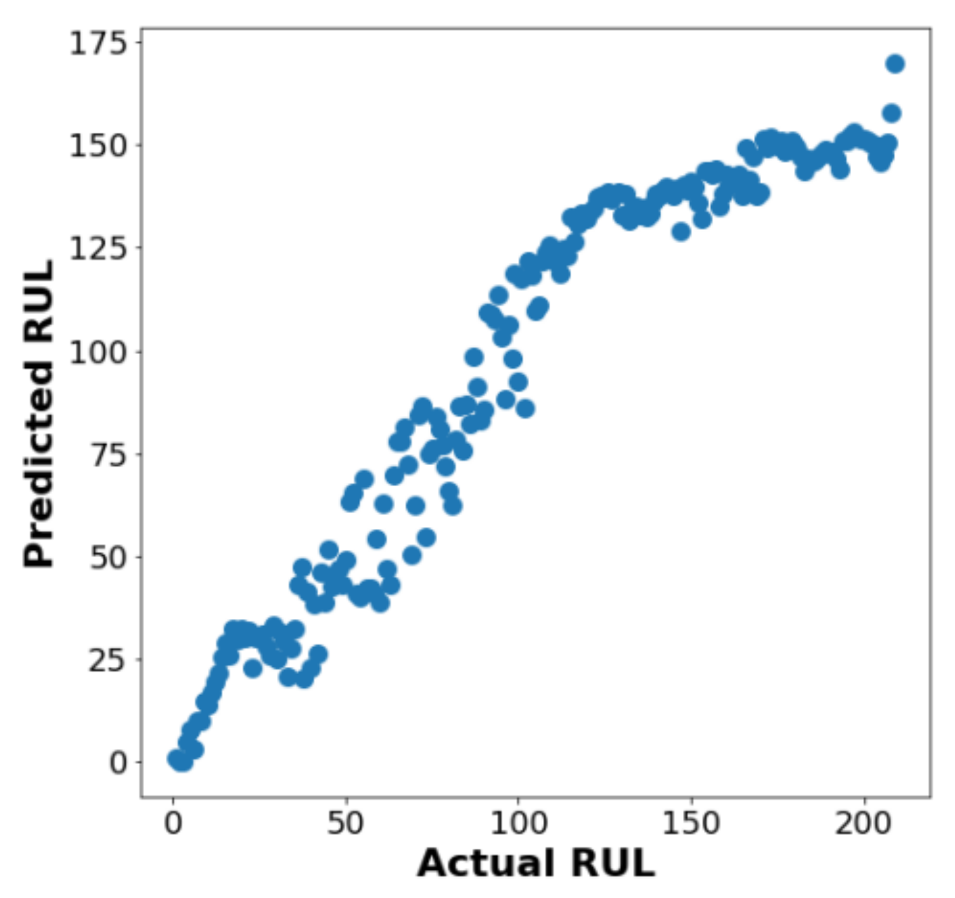
Cycle life and RUL prediction is a regression task. As there is no clear formula to describe the relationship between the proposed features and cycle numbers quantitatively, we chose symbolic regression (SR), a machine learning model complemented by the genetic programming optimization method, to solve this problem, because it could generate an expression close to the theoretical formula by progressive optimization. The model structure is shown in Figure 5. First, a series of initial functions are randomly generated to roughly fit the mathematical relationship between the proposed features and the RUL. Then, this algorithm allows these initial functions to breed, mutate, and evolve on account of the survival of the fittest. We used a Python library called gplearn to implement symbolic regression programming. Hyper-parameters (p_crossover = 0.5, p_subtree_mutation = 0.1, p_hoist_mutation = 0.2, p_point_mutation = 0.1) and function sets (‘add,’ ‘sub,’ ‘mul,’ ‘div,’ ‘sqrt,’ ‘log,’ ‘abs,’ ‘neg,’ ‘inv,’ ‘max,’ ‘min’) were adopted herein to obtain a brief but accurate description formula. The experimental setup of hyper-parameters in the SR model is shown in

Table 1. The experimental setup of hyper-parameters in SR model.

Parameter	Value
population size	5000
Generations	5
stopping criteria	0.01
p_crossover	0.7
p_subtree_mutation	0.1
p_hoist_mutation	0.05
p_point_mutation	0.1
function set	‘add’, ’sub’, ’mul’, ’div’, ’sqrt’, ’log’, ’abs’, ’neg’, ’inv’, ’max’, ’min’
parsimony coefficient	0.001

p_crossover is used to control the probability of mixing components between individual trees, while subtree will be replaced by a naïve random element during mutation, which is controlled by p_subtree_mutation. A high p_hoist_mutation number could avoid too complicated a formula, and p_point_mutation could bring opportunities for reintroducing eliminative functions and operators. The above probabilities were chosen to trade-off the complexity against the accuracy of formulas.

.

The coefficient of determination (R²) and root-mean-square error (RMSE) were chosen to evaluate the model performance. R² and RMSE are frequently chosen to evaluate the machine learning model performance [39,40]. R² could reflect the fitting degree of the regression equation, and the formula is as follows:

$$\begin{array}{c}{R}^2\left(y,\widehat{y}\right)=1-\frac{{{\displaystyle \sum }}_{i=0}^{n-1}{\left(y_i-{\widehat{y}}_i\right)}^2}{{{\displaystyle \sum }}_{i=0}^{n-1}{\left(y_i-\overline{y}\right)}^2}\end{array}$$

(5)

$$\overline{y}=\frac{1}{n}{{\displaystyle \sum }}_{i=0}^{n-1}{y}_i$$

(6)

where ${\widehat{y}}_i$ represents the predicted value of the ith sample, $y_i$ is the corresponding true value, and n denotes the number of samples. The best possible score is 1.0 and it would be negative if the model is arbitrarily worse. RMSE is defined as [4]:

$$RMSE=\sqrt{\frac{1}{n}{\displaystyle \sum }_{i=1}^n{\left(y_i-{\widehat{y}}_i\right)}^2}$$

(7)

where y_i is the observed cycle life, ŷ_i is the predicted cycle life, and n is the total number of samples.

3. Results

The battery dataset was collected when the discharge capacity of each battery decreased to 80% of the initial discharge capacity. The capacity of the batteries ranged from 40 to 60 mAh and the cycle lives ranged from 70 to 213 cycles. Figure 6 shows the discharge capacity as a function of cycle number for the whole cycle life, where the color denotes different batteries. The capacity fade speeds were different in the first few cycles and there were even some noisy fluctuations in the capacity fading curves.

We built a symbolic regression model using a series of descriptors extracted from the full voltage curves of each cycle. The specific feature selection and hyperparameter setup are discussed in the above section. After several populations of training, an optimized expression generated by our SR model outputted predicted values approaching the ground-truth RUL values in our training battery data. The formulas generated by our SR model can be found in

Table 2. The six mathematical formulas generated by the SR model.

Formulas	R2	Complexity
X5	0.7482	0
min(X29, X5)	0.7730	1
0.820 × X1	0.8768	1
min(X20, 0.848 × X1)	0.9093	2
max(X1, $\sqrt{\mathrm{X}24}$) × 24	0.7884	3
X5 × max($\sqrt{\mathrm{X}21}$, X6 − (X24/X21))	0.9307	5

. In addition, the pair plot for the actual RUL of the test batteries and the predicted RUL inferred by the fourth formula in Table 2 is shown in Figure 7.

The explanations of each symbol shown in Table 2 are as follows: X1 denotes charge-specific capacity; X5 and X6 represent the integrals of capacity and voltage charging/discharging curves, respectively; X20 is the kurtosis of difference between the charging and discharging curve; X21 describes the previous locally convex/concave X coordinate of the voltage and capacity charging curve; X24 denotes the latter locally convex/concave Y coordinate of the voltage and capacity charging curve; X29 is the charging time. ‘min()’ means taking the minimum value of elements. ’max()’ means taking the maximum value of elements. $R^2$ can be calculated by using Equations (5) and (6). The complexity is also the number of operational symbols that can measure the complexity of formulas in the case of overfitting.

The final equation obtained from the SR model is expressed as follows:

$$\min \left(\mathrm{X}20, 0.848\times \mathrm{X}1\right)$$

(8)

where X20 denotes the kurtosis of difference between the charging and discharging curve, and X1 represents the charge-specific capacity.

We also conducted a comparison of predicted results and errors with the other three machine-learning methods coming from recent excellent related studies in the literature: support vector regression (SVR), Gaussian process regression (GPR), and elastic net (EN), as shown in

Table 3. Comparison of RUL prediction results of GPR, SVR, EN, and SR (RUL_Error =|RUL_prediction – RUL_True|).

Method	R2	RMSE	RULError53 (RULTrue = 157)	RULError105 (RULTrue = 105)	RULError179 (RULTrue = 31)
SVR	0.81	26.50	2	6	27
GPR	0.83	24.64	23	7	13
EN	0.69	33.27	30	8	27
SR	0.91	18.17	4	4	0

. The RUL_prediction results for the SR model were calculated by the fourth formula in Table 2, and the other three were calculated by the methods in references [4,22,24], respectively. The computational characteristics for the four models are shown in

Table 4. The computational characteristics for the SR model.

Computational Characteristics	Value
	SVR	GPR	EN	SR
Training time	0.1800 s	3.1527 s	0.0021 s	13.2677 s
Inference time	0.0023 s	0.0078 s	0.0013 s	0.0017 s
Total used memory	0.5975 GB	0.5999 GB	0.5963 GB	0.6346 GB

. The explanation of each characteristic is as follows. Training time is the whole time for the training of our SR model, including 5 generations to breed, mutate, and evolve. Inference time is the time taken by the model from receiving the input battery feature parameters to calculating the predicted RUL values. Total used memory is the memory containing the model parameters and formulas of every generation.

4. Discussion

In this work, we successfully assembled 12 solid-state polymer batteries with cycle lives ranging from 70 to 213 cycles to build the training datasets. Then, we performed battery RUL prediction by using the symbolic regression method with 11 highly correlated features as model inputs. These 11 physical quantities, such as capacity, energy, and charge/discharge voltage differences, were designed and screened by analyzing their different degradation mechanisms and charging/discharging curves compared with liquid lithium batteries.

After populations of breed, mutation, and evolution training, a high number of formulas were generated. Among these formulas, only those with high accuracies and low complexities can be explained for researchers to better understand the relationship of solid-state batteries to their characteristics. The six mathematical formulas that met the criteria of simplicity and accuracy are shown in Table 2. The first formula, X5, is the integral of the capacity and voltage charging curve of each battery (measured in units of mWh), which represents the amount of energy charged into the battery. This value is more than just capacity because it also takes inner resistance into account. The increase in impedance will affect the voltage value of each capacity point on the charge/discharge curve, thus affecting the integral energy. It could roughly predict the value of RUL with the simplest form. The second formula, min(X29, X5), is the smaller value between charging time and integral energy. The charging time is proportional to the capacity because of the constant current charging operation. This formula shows that the battery capacity and energy will decrease with the decrease in its RUL. The third formula is the battery discharge capacity (measured in units of mAh) multiplied by a factor of 0.820, and it could basically predict the value of RUL. It proves that capacity degradation also takes up a major factor for the aging of solid-state batteries. The fourth formula, min (X20, 0.798 × X1), takes the smaller value between our proposed kurtosis feature and the discharge capacity multiplied by a factor. X20 is a measure of polarization degree, which is the kurtosis value of the charge/discharge voltage difference sequence. In addition, X20 monotonously decreases with the cycle numbers, as shown in Figure 3b, because the overpotential caused by polarization concentrates at the beginning and the end of the charge/discharge process in the early battery cycles, and then gradually fills the whole charge/discharge process. X1 is a measure of capacity degradation, as we discussed in the third formula. Taken together, it proves that capacity degradation and impedance evolution are both highly correlated factors in solid-state battery aging, which is consistent with our previous conjecture. The forms of the fifth and sixth formulas are more complicated and lose their original physical meaning after calculation. However, it can still be seen that the values of charging/discharging energy and capacity are directly proportional to the RUL and the values of resistance and polarization degree are inversely proportional to the RUL. However, these two formulas were abandoned because they did not meet the trade-off between accuracy and complexity. Therefore, the fourth formula, containing features X20 (kurtosis) and X1 (charge-specific capacity), was the best compromise between accuracy and complexity.

We further investigated the fourth formula in Table 2 by comparing the predicted RUL and the true value of all experimental cycles. As shown in Figure 7, the upper-right corner of the plot demonstrates the initial stage of battery cycling. At this stage, the predicted value was less than the actual value. This might be due to the absence of significant aging characteristics, and the model could not accurately predict the battery life from the selected features. The lower-left corner of the plot shows the end stage of the battery cycling, and the predicted value was slightly higher than the actual value at this time, which may have been caused by the rapid decline in various performance indicators [31]. In the middle of the chart, the accuracy of the model was the most satisfactory. The obvious aging characteristics shown by the batteries are convenient for the model to capture and predict. Basically, all the data points were concentrated on the diagonal of the pair plot, which shows that the predicted value was in good agreement with the actual value. Our model achieved an excellent prediction accuracy from the perspective of R² (0.91) and RMSE (18.17). Through appropriate pretraining on LFP solid battery data, the model also exhibited a passable transfer prediction ability for NMC solid battery data. These experimental results showed that the method developed in this paper is universal in the field of solid-state lithium batteries with different material systems.

Then, we compared our results with the other three methods, SVR, GPR, and elastic net, in Table 3. SVR is a nonparametric algorithm based on support vector machine, GPR is a kernel-based probabilistic model that predicts according to the similarity between samples, and elastic net is a regularized linear regression model. These three methods have been employed frequently in the recent literature, and they have achieved high accuracy. However, due to the existence of an internal fixed formula, they still have no satisfactory adaptability and applicability in different battery systems. For accuracy comparison during these machine-learning models, we randomly selected cycles 53, 105 and 179 as examples. As the number of cycles increased, the advantage of our model gradually became obvious. At cycle 179, the predicted RUL error led by SR reduced to 0, while the predicted RUL errors of SVR, GPR, and EN remained high at 27, 13, and 27, respectively. R² and RMSE were evaluated by comparison between the prediction RUL values of four methods and the true RUL values from whole cycles of the test battery.

The higher prediction accuracy of our SR model was attributed to the screened features, which accurately tracked the battery degradation and created highly correlated inputs for the SR model. The diversity of applied symbols broke the restriction of fixed expressions and was also helpful for better optimization results [41]. However, the computation cost might be the current limitation of this model, as listed in Table 4. Comparing the other three methods with the fixed mapping formula form, the training time and storage consumption of symbolic regression were larger. This can be improved by reducing the number of screened features and formula symbols using domain knowledge in future work. Besides, the training process is strongly dependent on the quality and quantity of battery testing data. Thus, we made our experimental data publicly available at Zenodo [42]. This should encourage other battery researchers to share their experimental data to promote the development of battery cycle life prediction research.

The promise of symbolic regression for fast and accurate battery RUL prediction was demonstrated in this work. RUL prediction would promote the development of cell pack balanced design and battery echelon utilization [7]. Battery cycle life estimation could also greatly shorten the electrochemical test time and could accelerate the optimization of battery material systems and manufacturing processes. Overall, RUL prediction could provide great prospects for battery application, management, and optimization in the future.

5. Conclusions

This paper focused on identifying degradation patterns and the RUL prediction of solid-state lithium polymer batteries by using domain knowledge features. First, 11 physical quantities such as capacity, energy, and charge/discharge voltage differences were chosen as input features by analyzing degradation mechanisms, charging/discharging curves, and correlations between features and RUL. Then, the RUL was estimated using a symbolic regression model, which showed that kurtosis and charge-specific capacity had strong correlations with RUL. Finally, the SR model showed a higher accuracy (R², 0.91) compared with the other three machine learning methods (SVR, GPR, and EN with R² as 0.81, 0.83, and 0.69, respectively). This improvement was attributed to the accurate tracking of battery aging by the proposed impedance evolution features and the successful optimization by the unique formula mining function of SR models. Solid-state lithium batteries are close to the gate of commercialization, and their RUL prediction will become of vital importance. Improving the RUL prediction model with higher accuracy, earlier estimation, and better interpretability is promising to further promote the large-scale applications of solid-state lithium batteries.

References

1. Dunn, B.; Kamath, H.; Tarascon, J.-M. Electrical energy storage for the grid: A battery of choices. Science 2011, 334, 928–935. [Google Scholar] [CrossRef] [PubMed] [Green Version]
2. Nykvist, B.; Nilsson, M. Rapidly falling costs of battery packs for electric vehicles. Nat. Clim. Chang. 2015, 5, 329–332. [Google Scholar] [CrossRef]
3. Schmuch, R.; Wagner, R.; Hörpel, G.; Placke, T.; Winter, M. Performance and cost of materials for lithium-based rechargeable automotive batteries. Nat. Energy 2018, 3, 267–278. [Google Scholar] [CrossRef]
4. Severson, K.A.; Attia, P.M.; Jin, N.; Perkins, N.; Jiang, B.; Yang, Z.; Chen, M.H.; Aykol, M.; Herring, P.K.; Fraggedakis, D.; et al. Data-driven prediction of battery cycle life before capacity degradation. Nat. Energy 2019, 4, 383–391. [Google Scholar] [CrossRef] [Green Version]
5. Janek, J.; Zeier, W.G. A solid future for battery development. Nat. Energy 2016, 1, 16141. [Google Scholar] [CrossRef]
6. Xu, L.; Tang, S.; Cheng, Y.; Wang, K.; Liang, J.; Liu, C.; Cao, Y.-C.; Wei, F.; Mai, L. Interfaces in Solid-State Lithium Batteries. Joule 2018, 2, 1991–2015. [Google Scholar] [CrossRef] [Green Version]
7. Tang, X.; Zou, C.; Wik, T.; Yao, K.; Gao, F. Run-to-Run control for active balancing of lithium iron phosphate battery packs. IEEE Trans. Power Electron 2020, 2, 1499–1512. [Google Scholar] [CrossRef] [Green Version]
8. Schuster, S.F.; Bach, T.; Fleder, E.; Müller, J.; Brand, M.; Sextl, G.; Jossen, A.J. New charging method to avoid nonlinear aging of Lithium-Ion Batteries. Energy Storage 2015, 1, 44–53. [Google Scholar] [CrossRef]
9. Schuster, S.F.; Brand, M.J.; Berg, P.; Gleissenberger, M.; Jossen, A.J. Lithium-ion cell-to-cell variation during battery electric vehicle operation. Power Sources 2015, 297, 242–251. [Google Scholar] [CrossRef]
10. Harris, S.J.; Harris, D.J.; Li, C.J. Failure statistics for commercial lithium ion batteries: A study of 24 pouch cells. Power Sources 2017, 342, 589–597. [Google Scholar] [CrossRef] [Green Version]
11. Butler, K.T.; Davies, D.W.; Cartwright, H.; Isayev, O.; Walsh, A. Machine learning for molecular and materials science. Nature 2018, 559, 547–555. [Google Scholar] [CrossRef]
12. Granda, J.M.; Donina, L.; Dragone, V.; Long, D.L.; Cronin, L. Controlling an organic synthesis robot with machine learning to search for new reactivity. Nature 2018, 559, 377–381. [Google Scholar] [CrossRef]
13. Raccuglia, P.; Elbert, K.C.; Adler, P.D.; Falk, C.; Wenny, M.B.; Mollo, A.; Zeller, M.; Friedler, S.A.; Schrier, J.; Norquist, A.J. Machine-learning-assisted materials discovery using failed experiments. Nature 2016, 533, 73–76. [Google Scholar] [CrossRef]
14. Segler, M.H.S.; Preuss, M.; Waller, M.P. Planning chemical syntheses with deep neural networks and symbolic AI. Nature 2018, 555, 604–610. [Google Scholar] [CrossRef] [Green Version]
15. Sha, W.; Guo, Y.; Yuan, Q.; Tang, S.; Zhang, X.; Lu, S.; Guo, X.; Cao, Y.; Cheng, S. Artificial Intelligence to Power the Future of Materials Science and Engineering. Adv. Intell. Syst. 2020, 2, 2070320. [Google Scholar] [CrossRef] [Green Version]
16. Sidorov, D.; Liu, F.; Sun, Y. Machine learning for energy systems. Energies 2020, 13, 4708. [Google Scholar] [CrossRef]
17. Phattara, K.; Yodo, N. A data-driven predictive prognostic model for lithium-ion batteries based on a deep learning algorithm. Energies 2019, 12, 660. [Google Scholar]
18. Chandran, V.; Patil, C.; Karthick, A.; Ganeshaperumal, D.; Rahim, R.; Ghosh, A. State of charge estimation of lithium-ion battery for electric vehicles using machine learning algorithms. World Electr. Veh. J. 2021, 12, 38. [Google Scholar] [CrossRef]
19. Sheikh, S.; Anjum, M.; Khan, M.; Hassan, S.; Khalid, H.; Gastli, A.; Lazhar, B. A battery health monitoring method using machine learning: A data-driven approach. Energies 2020, 13, 3658. [Google Scholar] [CrossRef]
20. Attia, P.M.; Grover, A.; Jin, N.; Severson, K.A.; Markov, T.M.; Liao, Y.H.; Chen, M.H.; Cheong, B.; Perkins, N.; Yang, Z.; et al. Closed-loop optimization of fast-charging protocols for batteries with machine learning. Nature 2020, 578, 397–402. [Google Scholar] [CrossRef] [Green Version]
21. Dai, H.; Zhao, G.; Lin, M.; Wu, J.; Zheng, G. A novel estimation method for the state of health of lithium-ion battery using prior knowledge-based neural network and Markov chain. IEEE Trans. Ind. Electron 2019, 66, 7706–7716. [Google Scholar] [CrossRef]
22. Liu, D.; Song, Y.; Li, L.; Liao, H.; Peng, Y. On-line life cycle health assessment for lithium-ion battery in electric vehicles. J. Clean. Prod. 2018, 199, 1050–1065. [Google Scholar] [CrossRef]
23. Zhou, D.; Li, Z.; Zhu, J.; Zhang, H.; Hou, L. State of health monitoring and remaining useful life prediction of lithium-ion batteries based on temporal convolutional network. IEEE Access 2020, 8, 53307–53320. [Google Scholar] [CrossRef]
24. Zhang, Y.; Tang, Q.; Zhang, Y.; Wang, J.; Stimming, U.; Lee, A.A. Identifying degradation patterns of lithium-ion batteries from impedance spectroscopy using machine learning. Nat. Commun. 2020, 11, 1706. [Google Scholar] [CrossRef]
25. Ramakumar, C.; Deviannapoorani, L.; Dhivya, L.; Shankar, S.; Murugan, R. Lithium garnets: Synthesis, structure, Li+ conductivity, Li+ dynamics and applications. Prog. Mater. Sci. 2017, 88, 325–411. [Google Scholar] [CrossRef]
26. Christensen, J.; Newman, J. Erratum: A mathematical model for the lithium-ion negative electrode solid electrolyte interphase. J. Electrochem. Soc. 2004, 151, A1977. [Google Scholar] [CrossRef] [Green Version]
27. Pinson, M.B.; Bazant, M.Z. Theory of sei formation in rechargeable batteries: Capacity fade, accelerated aging and lifetime prediction. J. Electrochem. Soc. 2012, 160, A243–A250. [Google Scholar] [CrossRef]
28. Yang, X.-G.; Leng, Y.; Zhang, G.; Ge, S.; Wang, C.-Y. Computational design and refinement of self-heating lithium-ion batteries. J. Power Sources 2017, 360, 28–40. [Google Scholar] [CrossRef]
29. Christensen, J.; Newman, J. Cyclable lithium and capacity loss in li-ion cells. J. Electrochem. Soc. 2005, 152, A818–A829. [Google Scholar] [CrossRef]
30. Zhang, Q.; White, R.E. Capacity fade analysis of a lithium ion cell. J. Power Sources 2008, 179, 793–798. [Google Scholar] [CrossRef]
31. Koerver, R.; Dursun, I.; Leichtwei, T.; Dietrich, C.; Zhang, W.; Binder, J.; Hartmann, P.; Zeier, W.; Janek, J. Capacity fade in solid-state batteries: Interphase formation and chemomechanical processes in nickel-rich layered oxide cathodes and lithium thiophosphate solid electrolytes. Chem. Mater. 2017, 29, 5574–5582. [Google Scholar] [CrossRef]
32. Kaneko, F.; Wada, S.; Nakayama, M.; Wakihara, M.; Koki, J.; Kuroki, S. Capacity fading mechanism in all solid-state lithium polymer secondary batteries using peg-borate/aluminate ester as plasticizer for polymer electrolytes. Adv. Funct. Mater. 2009, 19, 918–925. [Google Scholar] [CrossRef]
33. Nakayama, M.; Wada, S.; Kuroki, S.; Nogami, M. Factors affecting cyclic durability of all-solid-state lithiumpolymer batteries using poly(ethylene oxide)-based solid polymer electrolytes. Energy Environ. Sci. 2010, 3, 1995–2002. [Google Scholar] [CrossRef]
34. Tang, S.; Lan, Q.; Xu, L.; Liang, J.; Lou, P.; Liu, C.; Cao, L.M.Y.; Cheng, S. A novel cross-linked nanocomposite solid-state electrolyte with super flexibility and performance for lithium metal battery. Nano Energy 2020, 71, 104600. [Google Scholar] [CrossRef]
35. Koga, C.; Wada, S.; Nakayama, M. All solid-state lithium polymer secondary batteries using spinel Li4/3Ti5/3O4 as an active material. Electrochim. Acta. 2010, 55, 2561–2566. [Google Scholar] [CrossRef]
36. Luo, D.; Zeng, S.; Chen, J. A probabilistic linguistic multiple attribute decision making based on a new correlation coefficient method and its application in hospital assessment. Mathematics 2020, 8, 340. [Google Scholar] [CrossRef] [Green Version]
37. Ren, L.; Zhao, L.; Hong, S.; Zhao, S.; Wang, H.; Zhang, L. Remaining useful life prediction for lithium-ion battery: A deep learning approach. IEEE Access 2018, 6, 50587–50598. [Google Scholar] [CrossRef]
38. Kang, P.; Chen, Z. Aircraft classification method based on the kurtosis. Eng. J. 2019, 21, 7855–7859. [Google Scholar] [CrossRef]
39. Sha, W.; Li, Y.; Tang, S.; Tian, J.; Zhao, Y.; Guo, Y.; Zhang, W.; Zhang, X.; Lu, S.; Cao, Y.; et al. Machine learning in polymer informatics. InfoMat 2020, 3, 353–361. [Google Scholar] [CrossRef]
40. Zhang, D. A coefficient of determination for generalized linear models. Am. Stat. 2018, 71, 310–316. [Google Scholar] [CrossRef]
41. Weng, B.; Song, Z.; Zhu, R.; Yan, Q.; Sun, Q.; Grice, C.; Yan, Y.; Yin, W. Simple catalysis descriptor discovered by symbolic regression. Nat. Commun. 2020, 11, 3513. [Google Scholar] [CrossRef]
42. Yuancheng, C. Features values of Solid-State Lithium Battery datasets [Data set]. Zenodo 2021. [Google Scholar] [CrossRef]
Figure 1. Summary of causes of battery degradation.
Applsci 11 04671 g001
Figure 2. A typical discharge curve of a solid-state battery.
Applsci 11 04671 g002
Figure 3. The charge/discharge voltage difference sequence (a) and their kurtosis values decrease with cycle numbers (b).
Applsci 11 04671 g003
Figure 4. Heatmap based on correlation (left) and the diagram of correlation coefficient (right) between all the 30 available features and RUL. The importance of each feature can be observed visually.
Applsci 11 04671 g004
Figure 5. Structure of symbolic regression model.
Applsci 11 04671 g005
Figure 6. Cycle performance of LFP/NCM solid-state lithium polymer batteries: discharge capacity decreases with cycle numbers.
Applsci 11 04671 g006
Figure 7. The pair plot for predicted/actual RUL.
Applsci 11 04671 g007