A Novel 2D Model for Freezing Phase Change Simulation during Cryogenic Fracturing Considering Nucleation Characteristics

Abstract

A 2D computational fluid dynamics (CFD) model in consideration of nucleation characteristics (homogeneous/heterogeneous nucleation) using the volume of fluid (VOF) method and Lee model was proposed. The model was used to predict the process of a multiphase flow accompanied by freezing phase change during cryogenic fracturing. In this model, nucleation characteristic (homogeneous and heterogeneous nucleation) during the freezing process and the influence of the formed ice phase on the flowing behavior was considered. Validation of the model was done by comparing its simulation results to Neumann solutions for classical Stefan problem. The comparison results show that the numerical results are well consistent with the theoretical solution. The maximum relative differences are less than 7%. The process of multiphase flow accompanied by the freezing of water was then simulated with the proposed model. Furthermore, the transient formation and growth of ice as well as the evolution of temperature distribution in the computational domain was studied. Results show that the proposed method can better consider the difference between homogeneous nucleation in the fluid domain and heterogeneous nucleation on the wall boundary. Finally, the main influence factors such as the flow velocity and initial distribution of ice phase on the fracturing process were discussed. It indicates that the method enable to simulate the growth of ice on the wall and its effect on the flow of multiphase fluid.

1. Introduction

Cryogenic fracturing [1,2,3,4] is a waterless reservoir stimulation technique which uses cryogenic fluids such as liquid carbon dioxide and liquid nitrogen for fracturing purpose. The technique takes advantage of the effect of thermal shock which presents as a sharp thermal gradient introduced by the cryogen on the rocks. It could enhance the fractures initiation and propagation in the rock stratum, viz. enhancing fracturing. Recently, as the disadvantages of the conventional hydraulic fracturing technique (heavy water consumption, soil pollution, formation damage, etc.) are widely recognized, cryogenic fracturing is gaining an increasing attention in the field of petroleum engineering.

Quite a few researches on cryogenic fracturing [5,6,7,8,9,10,11,12,13,14,15,16,17,18,19,20] have been carried out by scholars and engineers, in which significant efforts are devoted to investigating the feasibility of cryogenic fracturing for engineering application and figuring out the damage mechanism of cryogenic fracturing. These works are largely comprised of experimental studies in the laboratory. The porous structure of the reservoir stratum makes the fracturing process complicated and it enhances the difficulty of investigation. Nuclear magnetic resonance (NMR) [7,8], scanning electron microscope (SEM) [9,10], computed tomography (CT) [11,12] are widely used to capture the micro-structural changes in the specimens. Fractures are characterized with the aid of acoustic transmission, pressure-decay measurements [12], which enables further quantitative analysis. A series of cryogenic quenching tests (into liquid nitrogen) of specimens [13,14] were conducted and the evolution of permeability (pore distribution) [15,16] and mechanical properties (elastic modulus, tensile/compressive strength) [9,17,18] were studied. It was found that liquid nitrogen could induce damage to the specimens more efficiently by comparing the methods such as air cooling and water cooling [10]. The strength and brittleness of the shale could be reduced through the treatment of liquid nitrogen cooling, and it could help in decreasing the initiation pressure of reservoir stimulation [19]. It was also revealed that a repeated cooling–heating treatment could be more favorable in fracturing in comparison to a single cooling treatment [4,7,8]. Various factors, such as the cooling rate, initial temperature of specimens, the water saturation of specimens, the period of freeze thaw cycle [4], are found to affect the fracturing effect. Besides the experimental works, attempts were made to introduce numerical methods into the research on cryogenic fracturing in recent studies. Alqahtani [21] simulated the cryogenic fracturing process in unconventional reservoirs and evaluated the effect of thermal stresses on fracture development. Yao and co-workers [20] simulated the cryogenic fracturing process in Niobrara shale sample with the modified TOUGH2-EGS. A numerical scheme was developed by Li and co-workers [14] which could simulate the temperature history and the rewetting front positions in a laboratory quenching test. Wu and co-workers [9] numerically analyzed the influences of the cooling rate on rock degradation by conducting a three dimensional simulation using ABAQUS.

Most of the previous researches are focusing on the mechanical changes in the reservoir stratum caused by cryogenic stimulation (initiation and propagation of fracture, rock deformation, evolution of permeability etc.). Nevertheless, only few attentions are aroused to the heat and mass transfer process during cryogenic fracturing. The heat and mass transfer during fracturing would significantly influence the temperature distribution in the reservoir, further affecting the occurrence of thermal shock. Consequently, the heat and mass transfer process would significantly influence the cryogenic fracturing process which should be carefully considered. In this work, displacement flow of the residual water in the stratum by the injected cryogenic fracturing fluid is considered. In this process, the residual water in the reservoir is constantly cooled down by the cryogenic fracturing fluid while flowing in the stratum pore channel, which further leads the residual water to freeze. The newly-formed ice is supposed to occupy the pore channel partly or completely, affecting the subsequent state of flow. In this case, the cold energy transferred in the stratum during fracturing would also be influenced. Additionally, large-scale ice blockage can result in local pressure rise in the reservoir, which could enhance the initiation and propagation of fractures. According to the above analysis, it is noted that the displacement flow of residual water by the cryogenic fracturing fluid would have profound influence on the fracturing process. The process is quite complicated in practice as the following physical processes are involved and worked together including miscible/immiscible displacement flow (depends on the type of fracturing fluid (liquid carbon dioxide, liquid nitrogen)), liquid–gas phase transition (vaporization of the fracturing fluid), liquid–solid phase transition (solidification of residual water), pore-scale flow. It is indicated by the literature survey that nearly no research has focused on such a displacement process by far.

Accordingly, a primary study on this freezing-coupling displacement process is carried out which introduces a newly developed numerical model to simulate the freezing process during the displacement flow. Due to the complexity of the actual process, simplifications as illustrated in Figure 1 were made as follows.

(1)

A 2D model is developed. The main purpose of this research is to qualitatively reflect the freezing process during the displacement process and the influence of the formed ice on the flow status in a numerical method. The 2D method is considered sufficient for achieving this goal. Moreover, compared with 3D simulation, 2D simulation could significantly reduce the time cost of calculation.

(2)

The effect of porous structure is neglected and immiscible displacement flow in a single passage is considered. The “single passage” simplification is made referring to the research works on pure displacement process [22,23,24,25,26,27,28], in which the essential feature of the displacement process could be reflected. The “immiscible displacement” simplification comes from the fact that as a candidate of the cryogenic fracturing fluid, liquid nitrogen (LN₂) is hardly soluble in water.

(3)

The influences due to vaporizing of the fracturing fluid and pore scale are neglected. This simplification is made in consideration of the complexity of the vaporization process and the capillary effect. Research works on freezing soil [29] were also referred to, where the influence of vapor component is neglected.

Based on the above simplifications, the major effort is spent on simulating the growth of ice phase and the influence of ice phase on the flow status during the displacement process (Figure 1c).

Research on this process is supposed to provide a method to predict the ice blockage pattern in the reservoir properly, which is necessary for a further prediction of the fracture development, pressure distribution, permeability evolution, thermal shock position, and other factors during fracturing. An improvement in the fracturing efficiency can then be expected.

2. Mathematical Formulations

During the displacement flow process along with the growth of ice phase as shown in Figure 1c, the phase interaction can be described as: During the displacement, the cryogenic fluid would push the water towards the forward wall boundaries, which can be implemented by simulating the fluid dynamics based on the N-S governing equations. Furthermore, the interface and the development of each fluid phase can be dealt using the volume of fluid (VOF) method [30]. Meanwhile, according to the cooling effect induced by the cryogenic fluid, the water near the wall would freeze. The process of cooling and freezing can be simulated by the energy conservation equation and phase-change model [31,32,33,34,35]. On the other hand, the newly generated ice phase should attach to the wall and block the development of multiphase fluid. In order to simulate the above process, a transient CFD model for 2D computational domain on the basis of the VOF method is proposed to simulate the process of multiphase flow (water and cryogenic fluid) involving liquid–solid phase transition (water–ice). Three phases including the primary phase (water), the secondary phase (ice), and the third phase (cryogenic fluid) are defined. Therein, the mass transfers among the multiphase through the surface are neglected in this method. The momentum, continuity, energy and VOF equations in the governing equations are solved. This model is also capable of handling the conduction-controlled solidification problem (the classical Stefan problem) by reducing the number of defined phases to 2 (water and ice) and eliminating the momentum equation. In modeling the phase change (forming and growth of ice), the Lee model [35] is used and the nucleation rate of the classical nucleation theory (CNT) [36,37,38,39] is innovatively introduced in the calculation of mass transfer rate between water and ice phase. As for the interaction between the fluid and the ice phase [40,41,42], The sponge-layer absorbing technique [41], by which the ice phase can be handled to be similar to solid and then can perform the blocking effect on the other phases of water and cryogenic fluid, is adopted to reflect the influence of the newly formed ice on the flow status (the fluid variables, such as velocity, pressure).

2.1. Governing Equations

The volume fraction (α) represents the composition of the control cell. Therein, α_i = 1 suggests the cell is fully occupied by the i phase, α_i = 0 indicates there are no i phase in the cell and 0 < α_i < 1 means that only part of the cell contains i phase. The heat transfer process during cryogenic fracturing includes three phases which are the water, ice, and cryogenic fluid, respectively.

For the tracking of interface (water–cryogenic fluid, water–ice), the VOF method in Euler–Euler multiphase system is adopted, in which the interface is tracked by solving volume fraction equations. In the present work, the volume fraction of the i^th phase can be calculated as [43,44]:

$$\frac{\partial {\alpha }_i}{\partial t}+\nabla ·({\alpha }_i{\overrightarrow{u}}_i)=S_{{\alpha }_i}$$

(1)

where S_αi is the source term of the ice phase, which is induced by the mass transfer during ice formation, and the details would be discussed in the following section. In the computational domain with n phases, the volume fractions of these phases can be referred to the following constraint:

$${\sum }_{i=1}^n{\alpha }_i=1 .$$

(2)

Therein, the fluid density in the cell can be expressed according to the volume fractions of the n phases:

$$\rho =\sum {\alpha }_i{\rho }_i .$$

(3)

The mass conservation equations of each phase are solved, and the continuity equation of the i^th phase could be written as:

$$\frac{\partial {\alpha }_i{\rho }_i}{\partial t}+\nabla ·({\alpha }_i{\rho }_i{\overrightarrow{u}}_i)=S_{m_i}$$

(4)

where ${\rho }_i$ and ${\overrightarrow{u}}_i$ represent the fluid density and the fluid velocity of the i^th phase, respectively. Furthermore, S_mi represents the mass source which equals to zero at the flow interface (water–cryogenic fluid) and equals to mass transfer rate at the water–ice interface. The formulation of the mass source is presented in Section 2.2.

In this case, the momentum equations are applied to model the flow behavior of various phases, which can be written as following for the i^th phase.

$$\frac{\partial {\rho }_i{\alpha }_i{\overrightarrow{u}}_i}{\partial t}+\nabla ·({\rho }_i{\alpha }_i{\overrightarrow{u}}_i{\overrightarrow{u}}_i)=-{\alpha }_i\nabla p+\nabla ·{\stackrel{=}{\tau }}_i+K_{ji}({\overrightarrow{u}}_j-{\overrightarrow{u}}_i)+S_{u_i}$$

(5)

where p is pressure, K_ji is interfacial drag coefficient, S_ui is the source term of the momentum induced by the mass transfer which would be given in the next section in details. Furthermore, $\stackrel{=}{\tau }$ is the tensor of the stress-strain and it is described as:

$${\stackrel{=}{\tau }}_i={\mu }_i{\alpha }_i(\nabla {\overrightarrow{u}}_i+\nabla {\overrightarrow{u}}_i^T)+{\alpha }_i\left({\omega }_i-\frac{2}{3}{\mu }_i\right)\nabla ·{\overrightarrow{u}}_i\stackrel{=}{I}$$

(6)

where $\stackrel{=}{I}$ is unit tensor. In all the cases described in this work, Reynolds number is not allowed to exceed the critical value as about 2000, suggesting that a laminar flow model is used for the simulation. The energy conservation equation of the i^th phase is expressed as:

$$\frac{\partial {\rho }_i{\alpha }_i{H}_i}{\partial t}+\nabla ·({\rho }_i{\alpha }_i{\overrightarrow{u}}_i{H}_i)=\nabla ·\left(k_i\nabla T_i\right)+S_{H_i}$$

(7)

where H represents specific enthalpy, k represents the thermal conductivity, T represents the fluid temperature, and S_Hi represents the heat source due to mass transfer which would be described in the next section.

As a result, the governing equations mentioned above constitute a time-dependent and space-dependent model for the physical problems of the temperature distribution, the fluid flow and the phase change of solid–liquid. The source terms in the governing equations are deduced by introducing the nucleation rate of classical nucleation theory (CNT) into the Lee model, which would be presented in detail in the next section.

2.2. Freezing Model

The mass transfer rate in the freezing process is derived as following. Moreover, the sponge-layer absorbing technique, which is used to handle the fluid variables of ice phase, is introduced.

2.2.1. Model of Phase Change

The source terms owing to the phase change in the VOF, mass, momentum, and energy equations are handled using Lee model (Lee, 1979) [35,45,46], which is a physical based model for phase change and it can be employed in conjunction with the VOF multiphase model.

The source term in the mass conservation equation can be defined from Lee’s work [35]. If T_s > T_sat (ice dissolving into water), the rate of mass transfer for ice phase can be expressed as:

$${\dot{m}}_{sl}={\lambda }_{sl}{\alpha }_s{\rho }_s \frac{T_s-T_{sat}}{T_{sat}}$$

(8)

For the current solidification process, the process of ice dissolving into water can be neglected. Thus, ${\dot{m}}_{sl}$ can be treated as zero in this work. Furthermore, if T_l < T_sat (water freezing into ice), the rate of mass transfer for water phase can be written as:

$${\dot{m}}_{ls}={\lambda }_{ls}{\alpha }_l{\rho }_l \frac{T_{sat}-T_l}{T_{sat}}$$

(9)

where ${\dot{m}}_{sl}$ and ${\dot{m}}_{ls}$ are the mass transfer rates from ice to water and from water to ice, respectively, whose units are kg/(m³s). The λ is the time relaxation parameter of phase change with the unit of 1/s, which would be presented in detail later, α represents the volume fraction, ρ represents the density (kg m⁻³), and T represents the temperature (K). The subscript “s” and “l” represent solid (ice) and liquid (water). T_sat is the freezing point and it is 273.15 K for phase change between water and ice. Therefore, the source terms of the governing Equation (4) are calculated as:

$$S_{m_i}=\{\begin{array}{cc}{\dot{m}}_{sl}-{\dot{m}}_{ls},\hfill & \hfill for water phase\\ {\dot{m}}_{ls}-{\dot{m}}_{sl},\hfill & \hfill for ice phase\end{array}$$

(10)

Then, the source term of the volume fraction for each phase is described as:

$$S_{{\alpha }_i}=\frac{S_{m_i}}{{\rho }_i} .$$

(11)

Furthermore, the momentum source can be written as:

$$S_{u_i}=\{\begin{array}{cc}{\dot{m}}_{sl}{\overrightarrow{u}}_l-{\dot{m}}_{ls}{\overrightarrow{u}}_s,\hfill & \hfill for water phase\\ {\dot{m}}_{ls}{\overrightarrow{u}}_s-{\dot{m}}_{sl}{\overrightarrow{u}}_l,\hfill & \hfill for ice phase\end{array}$$

(12)

where ${\overrightarrow{u}}_l$ and ${\overrightarrow{u}}_s$ are the fluid velocities of water and ice. Therein, the velocity of ice phase is treated as zero. Finally, the source term in the energy equation can be calculated as:

$$S_{h_i}=\{\begin{array}{cc}{\dot{m}}_{sl}{H}_L,\hfill & \hfill for water phase \\ {\dot{m}}_{ls}{H}_L,\hfill & \hfill for ice phase\end{array}$$

(13)

where H_L represents the latent heat induced by phase change between water and ice.

2.2.2. Calculation of the Mass Transfer Rate

Nucleation rate, a concept of the classical nucleation theory (CNT) which can reflect the icing capability of water, is introduced into the calculation of mass transfer rate during freezing in the present model. The parameter (J) provides the number of newly formed nuclei per cubic meter and per second, which is mathematically described as:

$$J=\frac{k_{B}T}{h}\exp \left(-\frac{\Delta g}{k_{B}T}\right)n_L\exp \left(-\frac{\Delta G^{*}}{k_{B}T}\right)$$

(14)

where T represents the water temperature, h represents Planck constant which equals to 6.626 × 10⁻³⁴ J·s, k_B represents Boltzmann constant which equals to 1.380 × 10⁻²³ J·K⁻¹, Δg represents the activation energy of water molecules passing through water and ice interface which is around 4.000 × 10⁻²⁰ J, n_L represents the number of water molecule in a water volume which is about 3.34 × 10²⁸ m⁻³. Furthermore, ΔG* reflects the variation of Gibbs function for the phase change between ice and water. Gibbs function can be described as [47,48]:

$$\Delta G^{*}=\frac{16\pi {\gamma }_{iw}^3{T}_{sat}^2 }{3H_{Lv}^2\Delta T^2}{\alpha }_{ey}$$

(15)

where γ_iw is the superficial free energy of the water–ice interface, H_Lv is latent heat per volume. Moreover, α_ey is the shape coefficient of nucleation and can be written as:

$${\alpha }_{ey}=\frac{2-3cos\theta +cos{\theta }^3 }{4}$$

(16)

where θ is the contact angle ranging from 0° to 180°. It is shown by Equation (14) to Equation (16) that the influence of the contact angle is considered in calculating the nucleation rate. As the other parameters are constant, the nucleation rate would gradually increase with the contact angle decreasing, which quantitatively reflects the change during nucleation from the uniform state to the inhomogeneous state. To reflect the effects of the contact angle on the variation of the mass transfer rate, a mathematical relationship between the relaxation time parameter λ in Equation (9) and the nucleation rate J is established, which is presented as:

$${\lambda }_{ls}=J{V}_l$$

(17)

where V_l is the volume of water in the cell. Then, Equation (9) can be rewritten as:

$${\dot{m}}_{ls}=J{V}_l{\alpha }_l{\rho }_l \frac{T_{sat}-T_l}{T_{sat}} .$$

(18)

Equation (17) is established on a simple idea that the nucleation rate and the volume of the water in which nucleation occurs would both influence the freezing rate. With the treatment shown by Equation (17), difference between homogeneous nucleation in the fluid domain (without solid surface) and heterogeneous nucleation on the solid wall can be reflected by the mass transfer rate obtained via Equation (18). Furthermore, the influence of the newly formed ice phase (treated as solid surface by specifying contact angle value for it) on the freezing process is also possible to be simulated using the newly proposed model, which is hard to be considered in previous models.

2.2.3. Treatment of Variables in the Cells with Ice Phase

The fluid variables (velocity, pressure) of ice cell are treated based on the theory of the sponge-layer absorbing technique [41,49,50]. For the cell including ice phase, the modified fluid velocities and pressure could be expressed as:

$$u_M=\left(1-{\alpha }_s\right)u_C$$

(19)

$$v_M=\left(1-{\alpha }_s\right) v_C$$

(20)

$$p_M=\left(1-{\alpha }_s\right)p_C$$

(21)

where u_C, v_C, and p_C are the calculated x-velocity, y-velocity and pressure. u_M, v_M, and p_M are the corrected values of x-, y-velocities and pressure. Furthermore, α_s is the volume fraction of ice phase. If α_s equals to 1, it suggests that the cell is fully occupied by the ice phase. In this case, the velocity and pressure would be zero.

2.3. The Setting of the Boundary Conditions in the Computational Domain

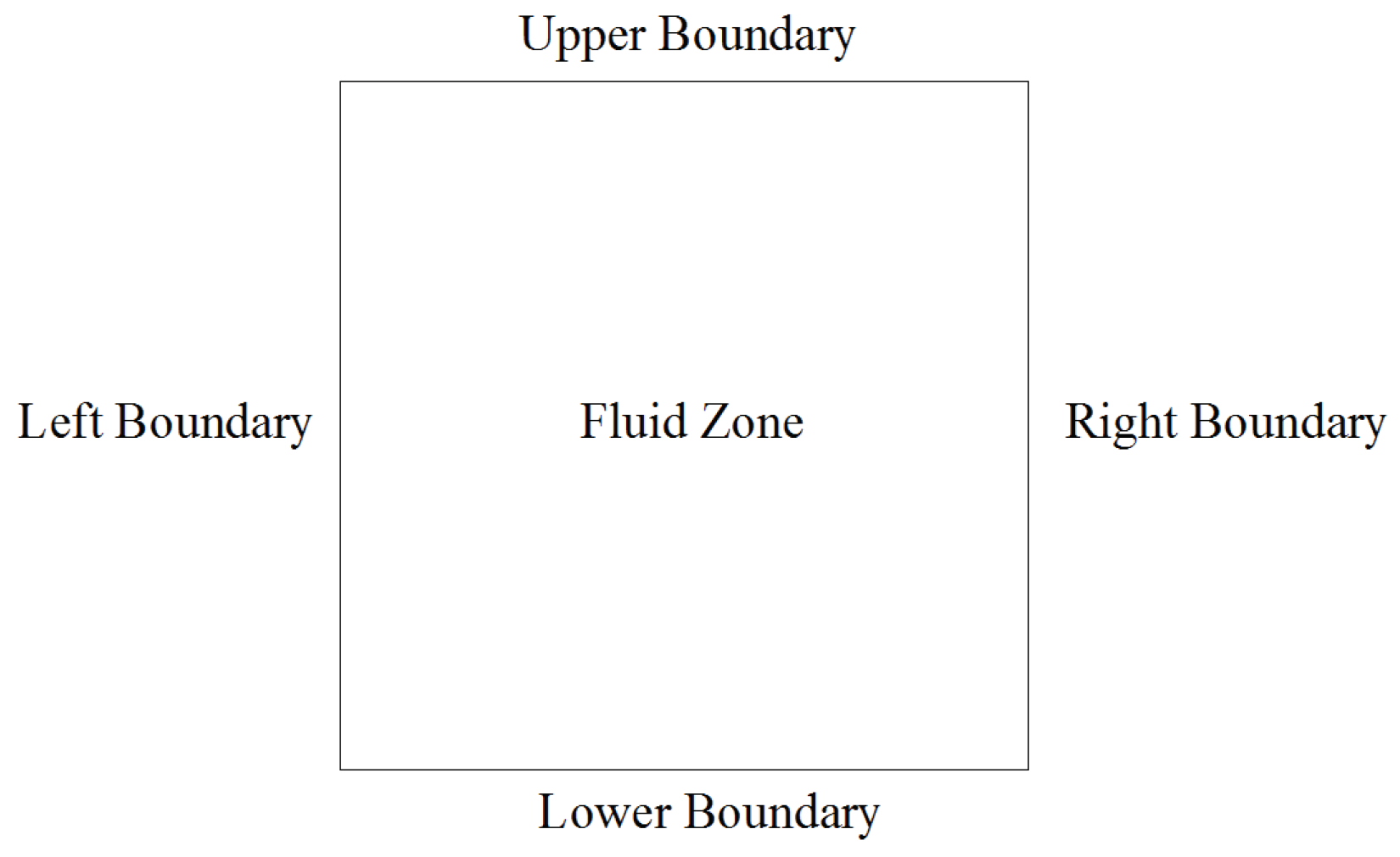
All the numerical studies are carried out in a two dimensional computational domain of 0.01 m × 0.01 m as shown in Figure 2.

The details of the boundary conditions applied in the case study are as follows:

(1) Velocity-inlet boundary

$$u_l=u_0, v_l=0,T_l=T_0,u_s=0,v_s=0,T_s=0,{\alpha }_s=0 .$$

(22)

(2) Outflow boundary

The flux of all the variables at the outflow boundary is set as zero, which means the state in the fluid zone are not affected by the conditions at the outflow boundary

$$\frac{\partial u_l}{\partial x}=0, \frac{\partial v_l}{\partial x}=0,\frac{\partial T_l}{\partial x}=0,\frac{\partial u_s}{\partial x}=0,\frac{\partial v_s}{\partial x}=0,\frac{\partial T_s}{\partial x}=0,\frac{\partial {\alpha }_s}{\partial x}=0 .$$

(23)

(3) Wall boundary with constant temperature

$$u_l=0, v_l=0,T_l=T_0,u_s=0,v_s=0,T_s=T_0,\frac{\partial {\alpha }_s}{\partial n}=0 .$$

(24)

(4) Adiabatic wall boundary

The heat flux passing through this face is set as zero:

$$u_l=0, v_l=0,\frac{\partial T_l}{\partial n}=0,u_s=0,v_s=0,\frac{\partial T_s}{\partial n}=0,\frac{\partial {\alpha }_s}{\partial n}=0 .$$

(25)

Different combinations of the above four boundary conditions are adopted in different cases, which are noted in the subsequent sections.

2.4. Solution Scheme of Numerical Model

On the basis of the second order upwind scheme, the governing equations of the mass, momentum, and temperature could be discretized. The SIMPLEC algorithm is selected as the solution method. Furthermore, the first order implicit solver is applied for time advancing in the unsteady simulation. The convergence criterions of all the variables are setting as 10⁻⁶. The above equations are solved in Fluent 6.3.26 CFD software. Finally, the calculation of the source terms in Section 2.2.1, Section 2.2.2 and Section 2.2.3 are carried out by defining the user defined function (UDF) in Fluent.

3. Results and Discussions

Here the sensitivities of mesh size and time step of the numerical model are discussed. The accuracy and feasibility of the present method are validated by comparing the simulation result with the Neumann solutions of Stefan problem. Thereafter, the influence factors such as the nucleation characteristics (homogeneous/heterogeneous) and the inlet flow on the freezing process are discussed.

3.1. Sensitivity Study and Model Validation

In this section, the classical Stefan problem [42,51,52] is simulated for model validation. Here the test cases with different mesh numbers (1600, 6400, and 25,600) and time steps (0.0005 s, 0.001 s, and 0.002 s) are designed to study the numerical convergence of the proposed method. The boundary conditions for model validation are listed in

Table 1. The settings of the boundary conditions (model validation).

Boundary	Conditions
Left	$u_l=0, v_l=0,T_l=253.15,u_s=0,v_s=0,T_s=253.15,\frac{\partial {\alpha }_s}{\partial n}=0$
Right	$u_l=0, v_l=0,\frac{\partial T_l}{\partial n}=0,u_s=0,v_s=0,\frac{\partial T_s}{\partial n}=0,\frac{\partial {\alpha }_s}{\partial n}=0$
Upper	$u_l=0, v_l=0,\frac{\partial T_l}{\partial n}=0,u_s=0,v_s=0,\frac{\partial T_s}{\partial n}=0,\frac{\partial {\alpha }_s}{\partial n}=0$
Lower	$u_l=0, v_l=0,\frac{\partial T_l}{\partial n}=0,u_s=0,v_s=0,\frac{\partial T_s}{\partial n}=0,\frac{\partial {\alpha }_s}{\partial n}=0$

.

Initial Conditions

The fluid zone of the computational domain is fully filled with liquid water with a temperature of 283.15 K (10 °C). The properties of water and ice are listed in

Table 2. Thermo-physical properties of water (0.5 °C, 0.1 MPa) and ice (0 °C) [53].

Materials	ρ (kg mz3)	Cp (J kg−1 K−1)	K (W m−1 K−1)	$\mathit{\mu }$
Water	996.32	4318	0.5263	0.00176
Ice	916.2	2050	2.22	-

. The numerical study in this paper is carried out at atmospheric pressure within a temperature range from −20 °C to 10 °C. It is assumed that the temperature variation would not induce the change of the thermo-physical properties of water and ice. The pressure variation during the simulation is also insignificant compared with atmospheric pressure. Therefore, the thermo-physical properties are set as constants.

In the numerical simulation, the volume fraction change of the ice phase indicates the formation and grow of the ice layer. There is no ice in the domain at the initial state, which suggests the volume fraction of ice phase would equal to zero in the whole domain. The ice would gradually form, leading to the volume fraction of the ice phase increase along with the time goes on. As the cell plotted in Figure 3 where the ice forms and develops, is adopted to demonstrate the ice layer. The ice–water interface is tracked by the changing of the volume fraction (ice phase) in the model. Then the location of the water–ice interface is determined as the contour of ice phase with the average value of volume fraction as 0.5. On this basis, the sensitivity test about the mesh number and time step for the conduction-controlled water–ice phase change problem is conducted and the result is plotted in Figure 4. Therein, the effect of mesh numbers (mesh schemes 1600, 6400, and 25,600) on the interface location evolution is given in Figure 4a. While, results for sensitivity tests of the time steps versus 0.0005 s, 0.001 s, and 0.002 s are plotted in Figure 4b, respectively. It is seen from Figure 4a that along with the mesh number increasing, the curves of the interfacial position evolution tend to coincide, indicating the convergence of the present method. In consideration of the computational accuracy and cost, the mesh number of 6400 (grid size 0.125 mm) and the time step of 0.001 s are suitable for the numerical simulation of freezing process in this work.

Furthermore, three values of the shape coefficient of nucleation α are selected (α_wall on the wall and α_ice on the ice are set to be the same as 0.01, 0.001, and 0.0001, respectively). The comparisons between the numerical results simulated by the present method and the Neumann solutions of the classical Stefan problem are presented in Figure 5 and Figure 6.

Figure 5 compares the result of interface position evolution by the present method (in three different α values) with that obtained through the theoretical Neumann solutions. It can be found from the figure that along with the shape coefficient of nucleation α decreasing, the numerical results of interfacial position evolution gradually tend to be the same and coincide well with the theoretical solutions. The max relative difference between the numerical results of α = 0.0001 and the theoretical solutions at various moments are about 6.58%.

Figure 6 shows the comparison of the temperature distribution at t = 6 s and 9 s obtained by the present method (α = 0.0001) and the theoretical Neumann solutions, respectively. It is found that the numerical result agrees well with the theoretical solutions and the max relative differences at 6 s and 9 s are about 4.01% and 4.74%, respectively. The comparison results in this section proved that the newly-proposed model could effectively predict the process of water freezing within a satisfying accuracy.

3.2. Discussion about Nucleation Characteristic and Inlet Flow

The multiphase flow process accompanied by solidification in a single flow passage (Figure 1c) is simulated. The phenomena of ice formation with different nucleation rates and the characteristic of multiphase flow around the ice phase are numerically studied, respectively. It should be noted that based on the grid size of 0.125 mm and the time step of 0.001 s from Figure 4, the courant number for the test cases with flow process in this section were analyzed and were less than 1, which can ensure the numerical iterative convergence. Thus, the grid size of 0.125 mm and the time step of 0.001 s are adopted in the subsequent test cases.

3.2.1. Influence of Homogeneous and Heterogeneous Nucleation Rates

Here two test cases of conduction-controlled water–ice phase change without inflow of cryogenic fluid (case 1, 2) are studied. For the simplified practical process as shown in Figure 1c, the left boundaries are designed to be inlet boundary to coincide with the situation of Figure 1c, and the temperatures on the inlet and wall boundaries are designed to be the same to study the difference of homogeneous and heterogeneous nucleation due to the different kinds of boundaries. Furthermore, different shape coefficients of nucleation are designed in Case 1 and 2 to distinguish the phase-change processes between the ice generation on the wall and the ice growth on the frozen ice, which should be closer to be practical situation. The boundary condition settings of Case 1 and 2 are listed in

Table 3. The settings of the boundary conditions (Case 1, 2).

Boundary	Conditions
Left	$u_l=0, v_l=0,T_l=253.15,u_s=0,v_s=0,T_s=253.15,{\alpha }_s=0$
Right	$\frac{\partial u_l}{\partial x}=0, \frac{\partial v_l}{\partial x}=0,\frac{\partial T_l}{\partial x}=0,\frac{\partial u_s}{\partial x}=0,\frac{\partial v_s}{\partial x}=0,\frac{\partial T_s}{\partial x}=0,\frac{\partial {\alpha }_s}{\partial x}=0$
Upper	$u_l=0, v_l=0,T_l=253.15,u_s=0,v_s=0,T_s=253.15,\frac{\partial {\alpha }_s}{\partial n}=0$
Lower	$u_l=0, v_l=0,T_l=253.15,u_s=0,v_s=0,T_s=253.15,\frac{\partial {\alpha }_s}{\partial n}=0$

.

Initial Conditions

The fluid zone of the computational domain is fully filled with liquid water with a temperature of 283.15 K (10 °C). The shape coefficients of nucleation α_ey on the velocity-inlet boundary and wall boundary are set to 1.0 and 0.1, respectively. It reflects the difference in nucleation characteristic at wall boundary and in the fluid. Meanwhile, in order to understand the influence of the shape coefficient of nucleation on ice formation and growth, different values of α_ice (shape coefficient on the ice) are specified with 0.1 in case 1 and 0.2 in case 2.

Simulation Results

For case 1, the distribution of ice phase at different moments are simulated and shown in Figure 7 to describe the process of ice growth. At the moment of t = 1.0 s which is shown by Figure 7a, due to the low temperature and high rate of crystallization J on the wall boundary, the ice phase firstly appears on the upper and lower boundaries. The formation of the ice at the wall boundary affects the J of water near the newly generated ice. Meanwhile, the low temperature of left boundary causes the formation of discontinuous loose ice near the velocity-inlet boundary. After a while, the form of ice phase on the three boundaries (upper, lower, and left) becomes regular and continuous at t = 5.0 s. With the time advancing, the ice phase gradually develops towards the interior of water area at t = 10.0 s. Therein, the ice layers on the upper and lower boundaries are always thicker than those on the left boundary. From Figure 7, it can be concluded that the phenomenon of ice formation and propagation can be well simulated by the numerical method. Moreover, by comparing the ice layer thickness on the left velocity-inlet boundary with that on the horizontal wall boundaries in Figure 7a, it is noted that the present method not only can consider the effect of the low temperature but also can reflect the difference between the rate of mass transfer due to homogeneous nucleation and heterogeneous nucleation for actual physical processes.

Figure 8 shows the distribution of ice phase at two moments (t = 1.0 s and t = 10.0 s) in case 2 which is simulated by the present method. By comparing these results to Figure 7, it can be found that the differences between case 1 (Figure 7) and case 2 (Figure 8) mainly present the freezing rate on the formed ice, which can be expressed as follows in detail. Firstly, near the left boundary, there is no continuous ice phase on the left boundary until t = 10.0 s in case 2. Secondly, during the whole process, the ice layers of case 2 on the upper and lower boundaries have less thickness than case 1. Therefore, the numerical method proposed in this paper is capable to consider the influences of different contact angles and different crystallization rates based on the practical situation.

Finally, temperature distribution at t = 10.0 s in both cases are simulated and plotted in Figure 9. It is seen that the range influenced by the boundaries with low temperature in the two cases are almost the same. On the other hand, the difference of the two cases mainly reflects the irregular oscillation of temperature at the location of the water–ice interface, which can show the distinct thermal conductivity of water and ice phase.

3.2.2. Interaction of Fluid Field and Ice Phase

In this section, the interaction between ice growth and fluid flow (case 3, 4, 5, and 6) is studied. For the practical situation, the cooling effect of the solid wall may be generally stronger than the formation water, which possibly causes the existence of the frozen ice at the initial moment of the displacement flow process. Furthermore, depending on the different conditions, the distributions of the initial frozen ice should be different. Therefore, four test cases with different initial ice phase are designed to study the displacement flow process with the growth of ice phase. The boundary conditions for case 3, 4, 5, and 6 are listed in

Table 4. The settings of the boundary conditions (Case 3, 4, 5, 6).

Boundary	Conditions
Left	$u_l=0.01, v_l=0,T_l=253.15,u_s=0,v_s=0,T_s=253.15,{\alpha }_s=0$
Right	$\frac{\partial u_l}{\partial x}=0, \frac{\partial v_l}{\partial x}=0,\frac{\partial T_l}{\partial x}=0,\frac{\partial u_s}{\partial x}=0,\frac{\partial v_s}{\partial x}=0,\frac{\partial T_s}{\partial x}=0,\frac{\partial {\alpha }_s}{\partial x}=0$
Upper	$u_l=0, v_l=0,T_l=253.15,u_s=0,v_s=0,T_s=253.15,\frac{\partial {\alpha }_s}{\partial n}=0$
Lower	$u_l=0, v_l=0,T_l=253.15,u_s=0,v_s=0,T_s=253.15,\frac{\partial {\alpha }_s}{\partial n}=0$

. The shape coefficients of nucleation α_ey in the fluid domain, on the ice and on the wall boundary are 1.0, 0.1, and 0.0001, respectively.

In the case study of the current section, the phase of cryogenic fluid is specified as n-hexanol (CH₃(CH₂)₅OH). This substance could exist as steady liquid form at −40 °C (Melting point: −52 °C, Boiling point: 157 °C). Moreover, its solubility in water is quite low (6 g/L, 25 °C). Considering the test conditions (below 0 °C most time), n-hexanol is an ideal choice for conducting the freezing-coupling immiscible displacement process with water. The thermal properties of n-hexanol is listed in

Table 5. Thermo-physical properties of n-hexanol (10 °C, 0.1 MPa) [54].

Materials	ρ (kg m−3)	Cp (J kg−1 K−1)	k (W m−1 K−1)	μ (Pas)
N-hexanol	814	2090	0.141	0.0052

.

Similar to those of water and ice, the thermo-physical properties of n-hexanol are set as constants in simulations.

Initial Conditions

To investigate the influence of the ice phase distribution on the flowing state, different distributions of the ice phase in the computational domain are specified as the initial conditions. To obtain the initial ice phase distribution data, a case of conduction-controlled water–ice phase change without any fluid inflow (case ex) is carried out with the boundary conditions listed in

Table 6. The settings of the boundary conditions (Case ex).

Boundary	Conditions
Left	$u_l=0, v_l=0,T_l=283.15,u_s=0,v_s=0,T_s=283.15,{\alpha }_s=0$
Right	$\frac{\partial u_l}{\partial x}=0, \frac{\partial v_l}{\partial x}=0,\frac{\partial T_l}{\partial x}=0,\frac{\partial u_s}{\partial x}=0,\frac{\partial v_s}{\partial x}=0,\frac{\partial T_s}{\partial x}=0,\frac{\partial {\alpha }_s}{\partial x}=0$
Upper	$u_l=0, v_l=0,T_l=253.15,u_s=0,v_s=0,T_s=253.15,\frac{\partial {\alpha }_s}{\partial n}=0$
Lower	$u_l=0, v_l=0,T_l=253.15,u_s=0,v_s=0,T_s=253.15,\frac{\partial {\alpha }_s}{\partial n}=0$

.

Initial condition in Case ex is set as: The fluid zone of the computational domain is fully filled with liquid water with a temperature of 283.15 K (10 °C).

The main difference between case ex and case 1, 2 is that the temperature at left boundary is set as 283.15 K (10 °C). Therefore, the ice phase in case ex would only form and grow on the two horizontal boundaries (upper and lower). Different situations of initial ice phase distribution are obtained by importing the data of ice phase distribution at different moments in case ex into the current study cases. For this time, ice distribution at t = 50 s, 100 s, and 150 s in case ex is adopted and the distribution state in the computational domain is shown by Figure 10.

Besides the above three initial ice phase distribution conditions, the case where there is no initial ice phase is also considered. Accordingly, four cases are included in the case study in this section. The initial ice phase distributions of the four cases are:

(1) Case 3 (no initial ice phase),

(2) Case 4 (Figure 10a),

(3) Case 5 (Figure 10b), and

(4) Case 6 (Figure 10c).

The part that is not occupied by the ice phase in the computational domain is filled with liquid water at beginning with a temperature of 283.15 K (10 °C).

Simulation Results

Firstly, in case 3 at the initial stage (t = 0.0 s), there is no ice in the computational domain. By the method of this paper, the process of n-hexanol driving water and ice developing is numerically simulated, and then the distributions of cryogenic fluid, water, and ice at different moments are presented in Figure 11. The red zone represents the cryogenic fluid and ice, and the blue zone represents the water phase. From the figure, it is seen that the numerical simulation method could simulate the process of ice expansion and two-phase fluid flow. At the initial phase of t = 0.2 s, due to the low temperature and high rate of crystallization on the wall boundary, there are respective ice layers on the upper and lower boundaries. Then the cryogenic fluid of n-hexanol from the left velocity-inlet boundary flows around the ice layers and drives the water in the middle domain. Furthermore, the low temperature of n-hexanol affects the growth of ice on the wall boundaries and causes the left of the ice layer to be thicker. With time advancing (t = 0.4 s, 0.6 s, and 0.8 s), the ice layers gradually grow and further block the inflow of cryogenic fluid. Then the n-hexanol flows through the narrow channel due to the formed ice and then spreads towards the whole water area.

The flow fields distribution at various moments are shown in Figure 12. The influences of the ice layer on the flow state are reflected in the flow velocity changing (a value of up to about 0.014 m s⁻¹ is obtained in the simulation, which is higher than the inlet velocity of 0.01 m s⁻¹, indicating the fluid acceleration due to the presence of ice layer). For the fluid in the right domain with the thinner ice layers, the fluid velocity gradually decreases and becomes relatively stable. The velocity distribution shown in Figure 12 indicates that the simulated result obeyed the basic conservation law of mass and momentum. Thus, the present method can correctly simulate the propagation of the ice phase and its effect on the flow state.

In order to study the effect of the initial distribution of the ice phases on the convection process, the distributions of three phases (cryogenic fluid, water and ice) at t = 0.5 s are plotted in Figure 13. Therein, case 3 is without initial ice and the initial ice phase distributions in case 4, case 5, and case 6 are presented in Figure 10a–c, respectively. It is obviously seen from Figure 13 that the initial ice phase distribution has significant influence on the convection of cryogenic fluid and water. With the initial ice phase composition increasing, the cryogenic fluid spreads more rapidly. Figure 14 shows the vector graph of fluid velocity of water and n-hexanol at t = 0.5 s under different initial conditions of ice phase composition. It also can be found from Figure 14 that as the initial ice phase composition increases, the fluid domain becomes narrower, which causes the max fluid velocity of two-phase fluid to increase and change from 0.013 m s⁻¹ to 0.032 m s⁻¹. Furthermore, Figure 15 describes the pressure distribution in the fluid domain. It can be found from Figure 15 that there are two peak values of pressure about 1.2~1.4 Pa which locate at the top-left corner and bottom-left corner due to the blockage of ice layers. From above analysis, it can be concluded that the present method enable the numerical simulation of the multiphase flow propagation accompanied by solidification phase change during cryogenic fracturing.

4. Conclusions

In this paper, a 2D numerical model considering the nucleation characteristics based on VOF method and Lee model is developed to predict the propagation of multiphase flow accompanied by solidification phase change during cryogenic fracturing. The formation and propagation of ice on the wall boundary along with multiphase flow around ice was studied. Conclusions are drawn as follows:

(1)

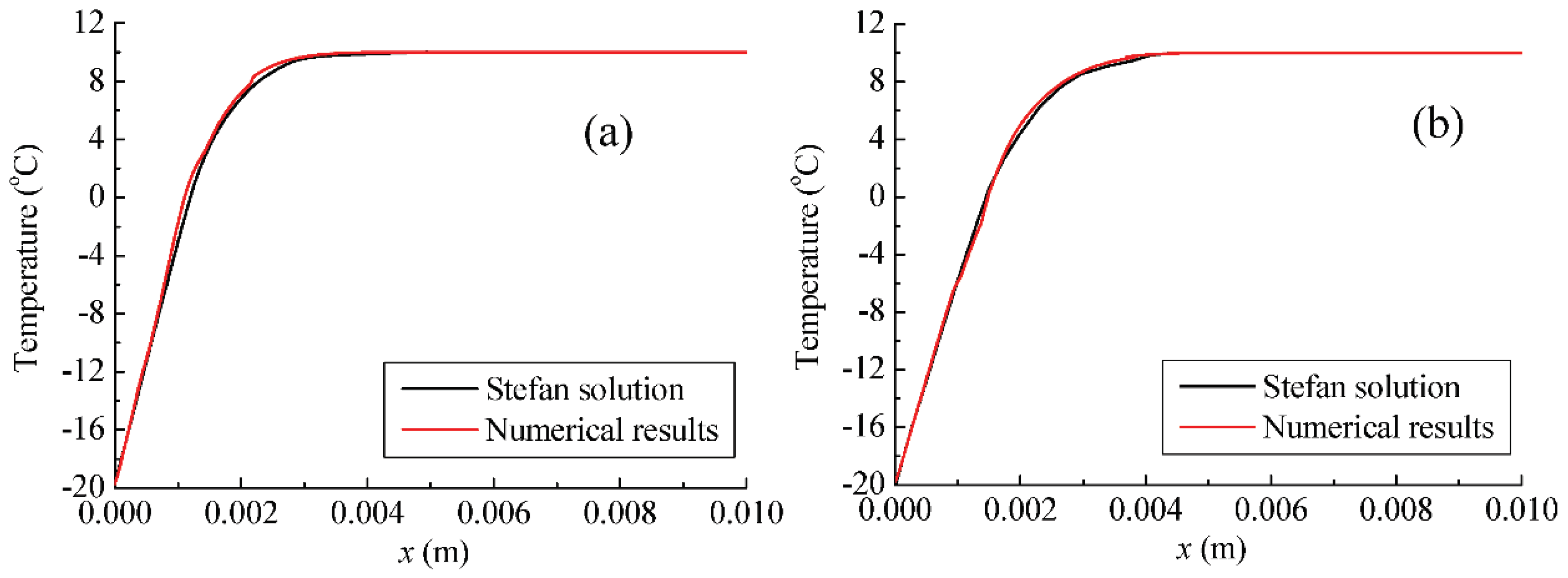
For the classical Stefan problem, the max relative difference between the convergent numerical results and the theoretical solutions are about 6.58%, which can validate the feasibility and accuracy of the newly proposed method.

(2)

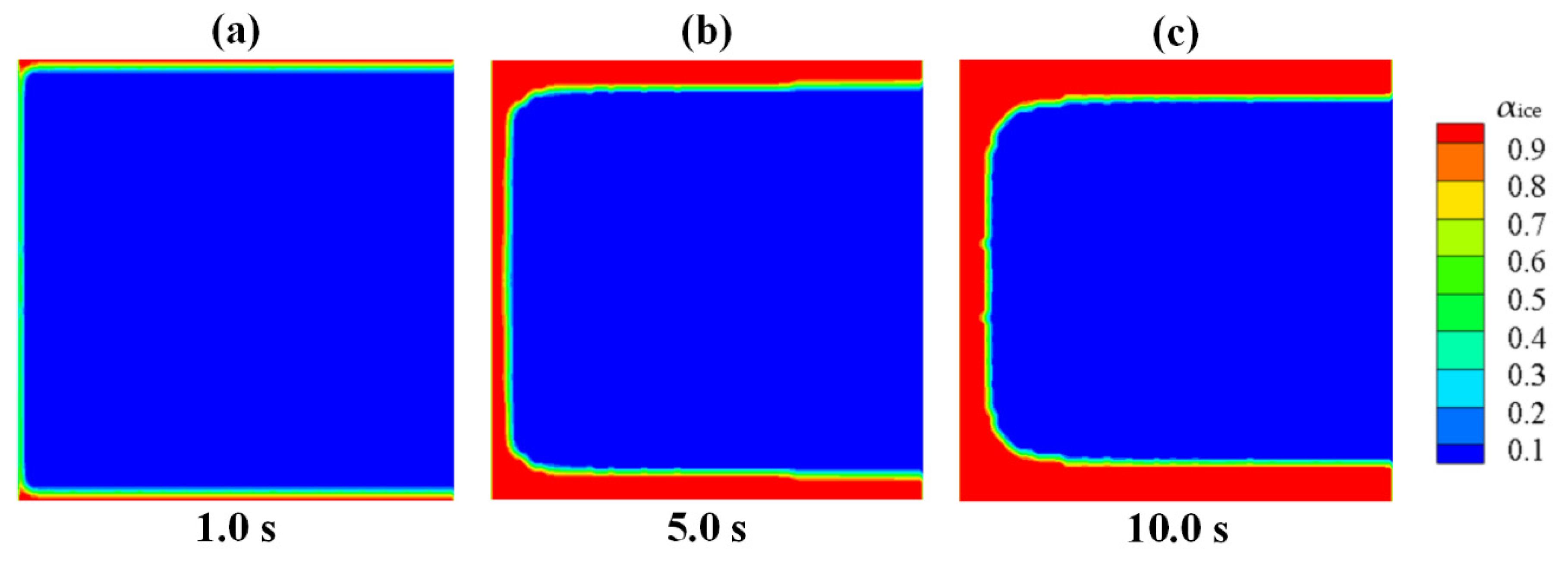
Through the simulation on the process of the ice generation and growth in Case 1, the improved Lee model in the proposed numerical method could consider the effect of low-temperature boundary on the freezing. It also could well reflect the different characteristic of the homogeneous nucleation and the heterogeneous nucleation on various kinds of boundaries.

(3)

By comparing the numerical solutions of Case 1 with that of Case 2, the concept of shape coefficient of nucleation in the proposed numerical method has the ability to distinguish the phase-change processes between the ice generation on the wall and the ice growth on the frozen ice, which could restore the practical situation.

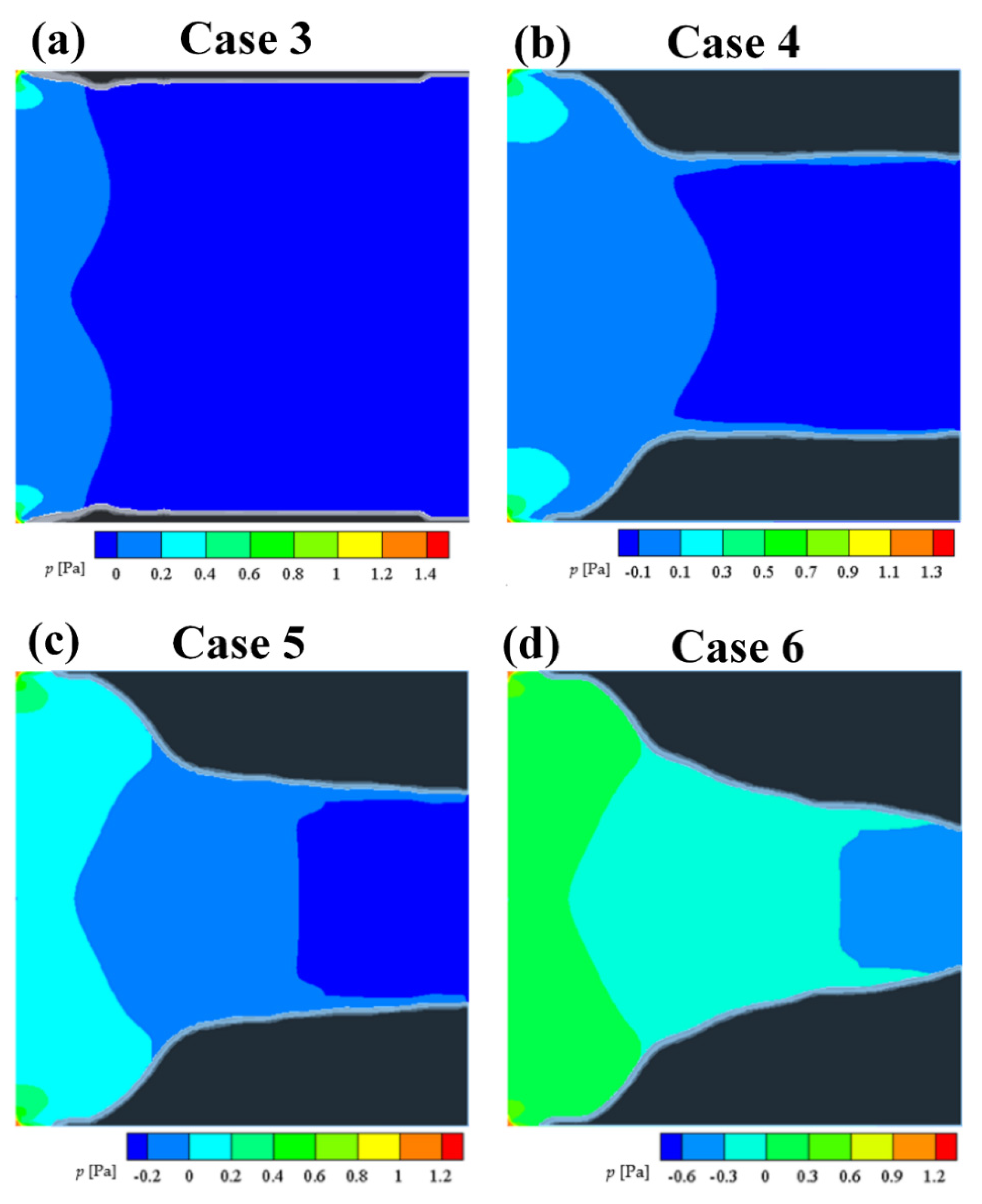
(4)

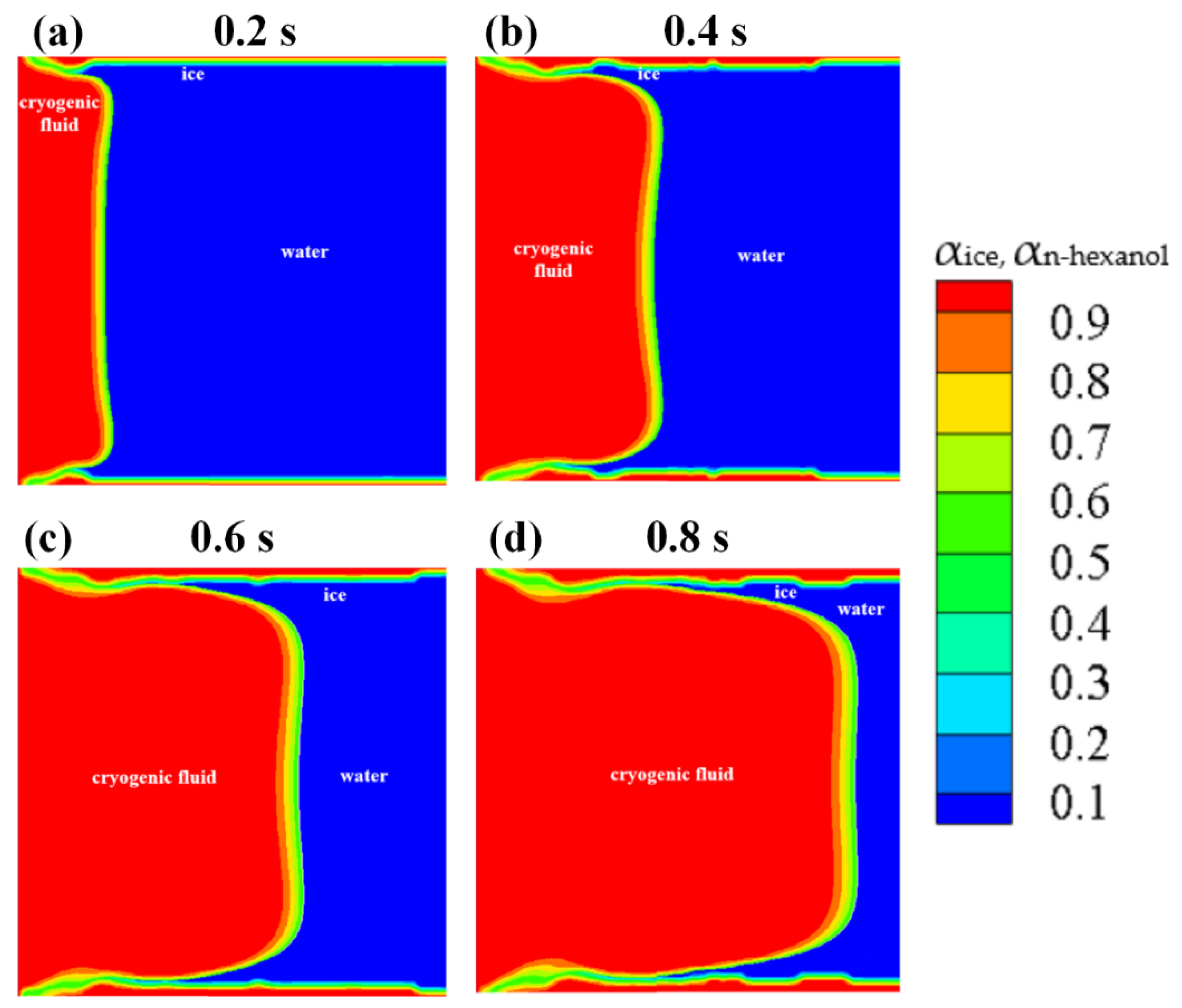
The numerical results of Case 3~6 indicate that the sponge-layer absorbing technique is capable of handling the frozen ice and simulating its blocking effect on fluid flow.

In future researches, the model experiments should be carried out to further validate the newly proposed numerical method. Furthermore, the method can be developed further on the following aspects: Considering the effects of temperature and pressure on the thermo-physical properties (thermal conductivity, density, viscosity, specific heat capacity, etc.) to meet the practical engineering requirements; extending the present method to three dimensions for more extensive application about the practical engineering problems; further performing the complete uncertainty analysis based on the experimental results; and further introducing more interactive effects among the multiphase fluids (such as mass transfer).

References

1. Li, Z.; Xu, H.; Zhang, C. Liquid nitrogen gasification fracturing technology for shale gas development. J. Pet. Sci. Eng. 2016, 138, 253–256. [Google Scholar] [CrossRef]
2. Zhang, Y. Study on Liquid Nitrogen Fracturing in Coalbed Gas Well. Master’s Thesis, Southwest Peroleum University, Chengdu, China, 2015. [Google Scholar]
3. Wang, L.; Yao, B.; Cha, M.; Alqahtani, N.B.; Patterson, T.W.; Kneafsey, T.J.; Miskimins, J.L.; Yin, X.; Wu, Y.S. Waterless fracturing technologies for unconventional reservoirs-opportunities for liquid nitrogen. J. Nat. Gas Sci. Eng. 2016, 35, 160–174. [Google Scholar] [CrossRef] [Green Version]
4. Huang, Z.; Zhang, S.; Yang, R.; Wu, X.; Li, R.; Zhang, H.; Hung, P. A review of liquid nitrogen fracturing technology. Fuel 2020, 266, 117040. [Google Scholar] [CrossRef]
5. Grundmann, S.R.; Rodvelt, G.D.; Dials, G.A. Cryogenic nitrogen as a hydraulic fracturing fluid in the Devonian shale. In Proceedings of the SPE Eastern Regional Meeting, Pittsburgh, PA, USA, 9–11 November 1998. [Google Scholar]
6. McDaniel, B.W.; Grundmann, S.R.; Kendrick, W.D. Field applications of cryogenic nitrogen as a hydraulic-fracturing fluid. J. Pet. Technol. 1998, 50, 5038–5039. [Google Scholar]
7. Qin, L.; Zhai, C.; Liu, S.; Xu, J.; Wu, S.; Dong, R. Fractal dimensions of low rank coal subjected to liquid nitrogen freeze-thaw based on nuclear magnetic resonance applied for coalbed methane recovery. Powder Technol. 2018, 325, 11–20. [Google Scholar] [CrossRef]
8. Qin, L.; Zhai, C.; Liu, S.; Xu, J.; Yu, G.; Sun, Y. Changes in the petrophysical properties of coal subjected to liquid nitrogen freeze-thaw-A nuclear magnetic resonance investigation. Fuel 2017, 194, 102–114. [Google Scholar] [CrossRef]
9. Wu, X.; Huang, Z.; Li, R.; Zhang, S.; Wen, H.; Huang, P.; Dai, X.; Zhang, C. Investigation on the damage of high-temperature shale subjected to liquid nitrogen cooling. J. Nat. Gas Sci. Eng. 2018, 57, 284–294. [Google Scholar] [CrossRef]
10. Wu, X.; Huang, Z.; Song, H.; Zhang, S.; Cheng, Z.; Li, R.; Wen, H.; Huang, P.; Dai, X. Variations of Physical and Mechanical Properties of Heated Granite After Rapid Cooling with Liquid Nitrogen. Rock Mech. Rock Eng. 2019, 52, 2123–2139. [Google Scholar] [CrossRef]
11. Cha, M.; Yin, X.; Kneafsey, T.; Johanson, B.; Alqahtani, N.; Miskimins, J.; Patterson, T.; Wu, Y.S. Cryogenic fracturing for reservoir stimulation-Laboratory studies. J. Pet. Sci. Eng. 2014, 124, 436–450. [Google Scholar] [CrossRef] [Green Version]
12. Cha, M.; Alqahtani, N.B.; Yin, D.; Kneafsey, T.J.; Yao, B.; Wu, Y. Laboratory system for studying cryogenic thermal rock fracturing for well stimulation. J. Pet. Sci. Eng. 2017, 156, 780–789. [Google Scholar] [CrossRef] [Green Version]
13. Li, R.; Huang, Z.; Wu, X.; Yan, P.; Dai, X. Cryogenic quenching of rock using liquid nitrogen as a coolant: Investigation of surface effects. Int. J. Heat Mass Transf. 2018, 119, 446–459. [Google Scholar] [CrossRef]
14. Li, R.; Zhang, C.; Huang, Z. Quenching and rewetting of rock in liquid nitrogen: Characterizing heat transfer and surface effects. Int. J. Therm. Sci. 2020, 148, 106161. [Google Scholar] [CrossRef]
15. Zhao, B.; Zhang, G.Q.; Zhao, P.Y.; Wang, L.L.; Lin, Y.; Lv, Y.J. Experimental study of mechanics and seepage characteristics of sandstones after liquid-nitrogen stimulation. J. Nat. Gas Sci. Eng. 2017, 47, 11–21. [Google Scholar] [CrossRef]
16. Yin, G.; Shang, D.; Li, M.; Huang, J.; Gong, T.; Song, Z.; Deng, B.; Liu, C.; Xie, Z. Permeability evolution and mesoscopic cracking behaviors of liquid nitrogen cryogenic freeze fracturing in low permeable and heterogeneous coal. Powder Technol. 2018, 325, 234–246. [Google Scholar] [CrossRef]
17. Han, S.; Cheng, Y.; Gao, Q.; Yan, C.; Han, Z. Experimental study of the effect of liquid nitrogen pretreatment on shale fracability. J. Nat. Gas Sci. Eng. 2018, 60, 11–23. [Google Scholar] [CrossRef]
18. Gao, F.; Cai, C.; Yang, Y. Experimental research on rock fracture failure characteristics under liquid nitrogen cooling conditions. Results Phys. 2018, 9, 252–262. [Google Scholar] [CrossRef]
19. Jiang, L.; Cheng, Y.; Han, Z.; Gao, Q.; Yan, C.; Wang, H.; Fu, L. Effect of liquid nitrogen cooling on the permeability and mechanical characteristics of anisotropic shale. J. Pet. Explor. Prod. Technol. 2019, 9, 111–124. [Google Scholar] [CrossRef] [Green Version]
20. Yao, B.; Wang, L.; Yin, X.; Wu, Y.S. Numerical modeling of cryogenic fracturing process on laboratory-scale Niobrara shale samples. J. Nat. Gas Sci. Eng. 2017, 48, 169–177. [Google Scholar] [CrossRef]
21. Alqahtani, N.B. Experimental Study and Finite Element Modeling of Cryogenic Fracturing in Unconventional Reservoirs. Ph.D. Thesis, Colorado School of Mines, Golden, CO, USA, 2015. [Google Scholar]
22. Dong, B.; Yan, Y.; Li, W.; Song, Y. Lattice Boltzmann simulation of viscous fingering phenomenon of immiscible fluids displacement in a channel. Comput. Fluids 2010, 39, 768–779. [Google Scholar] [CrossRef]
23. Freitas, J.F.; Soares, E.J.; Thompson, R.L. Residual mass and flow regimes for the immiscible liquid-liquid displacement in a plane channel. Int. J. Multiph. Flow 2011, 37, 640–646. [Google Scholar] [CrossRef]
24. Huang, J.; Xial, F.; Yin, X. Lattice Boltzmann Simulation of pressure-driven two-phase flows in capillary tube and porous medium. Comput. Fluids 2017, 155, 134–145. [Google Scholar] [CrossRef]
25. Caliman, H.M.; Soares, E.J.; Thompson, R.L. An experimental investigation on the Newtonian-Newtonian and viscoplastic-Newtonian displacement in a capillary tube. J. Non-Newton. Fluid Mech. 2017, 247, 207–220. [Google Scholar] [CrossRef]
26. Eslami, A.; Frigaard, I.A.; Taghavi, S.M. Viscoplastic fluid displacement flows in horizontal channels: Numerical simulations. J. Non-Newton. Fluid Mech. 2017, 249, 79–96. [Google Scholar] [CrossRef]
27. Soori, T.; White, A.R.; Ward, T. Immiscible fluid displacement in a porous media: Effect of surfactants introduced ab initio versus surfactants formed in-situ. J. Pet. Sci. Eng. 2019, 180, 310–319. [Google Scholar] [CrossRef]
28. Oladosu, O.; Bhakta, J.; Alba, K. Density-stable yield-stress displacement flow of immiscible fluids in inclined pipes. J. Non-Newton. Fluid Mech. 2020, 275, 104203. [Google Scholar] [CrossRef]
29. Song, W.; Zhang, Y.; Li, B.; Fan, X. A lattice Boltzmann method for heat and mass transfer phenomena with phase transformations in unsaturated soil during freezing process. Int. J. Heat Mass Transf. 2016, 94, 29–38. [Google Scholar] [CrossRef]
30. Hirt, C.W.; Nichols, B.D. Volume of Fluid (VOF) Method for the Dynamics of Free Boundaries. J. Comput. Phys. 1981, 39, 201–225. [Google Scholar] [CrossRef]
31. Nazzi Ehms, J.H.; De Césaro Oliveski, R.; Oliveira Rocha, L.A.; Biserni, C.; Garai, M. Fixed Grid Numerical Models for Solidification and Melting of Phase Change Materials (PCMs). Appl. Sci. 2019, 9, 4334. [Google Scholar] [CrossRef] [Green Version]
32. Voller, V.R. Modeling Solidification Processes; Technical Report, Mathematical Modeling of Metals Processing Operations Conference; American Metallurgical Society: Palm Desert, CA, USA, 1987. [Google Scholar]
33. Voller, V.R. A Computational Modeling Framework for the Analysis of Metallurgical Solidification Process and Phenomena; Technical Report, Conference for Solidification Processing; Ranmoor House: Sheffield, UK, September 1987. [Google Scholar]
34. Voller, V.R.; Prakash, C. A Fixed-Grid Numerical Modeling Methodology for Convection- Diffusion Mushy Region Phase-Change Problems. Int. J. Heat Mass Transf. 1987, 30, 1709–1720. [Google Scholar] [CrossRef]
35. Lee, W.H. A Pressure Iteration Scheme for Two-Phase Modeling; Technical Report LA-UR, 79-975; Los Alamos Scientific Laboratory: Los Alamos, NM, USA, 1979. [Google Scholar]
36. Ickes, L.; Welti, A.; Hoose, C.; Lohmann, U. Classical nucleation theory of homogeneous freezing of water: Thermodynamic and kinetic parameters. Phys. Chem. Chem. Phys. 2015, 17, 5514–5537. [Google Scholar] [CrossRef]
37. Němec, T. Estimation of ice–water interfacial energy based on pressure-dependent formulation of classical nucleation theory. Chem. Phys. Lett. 2013, 583, 64–68. [Google Scholar] [CrossRef]
38. Sear, R.P. Nucleation: Theory and applications to protein solutions and colloidal suspensions. J. Phys. Condens. Matter 2007, 19, 033–101. [Google Scholar] [CrossRef]
39. Wilson, P.W.; Heneghan, A.F.; Haymet, A.D.J. Ice nucleation in nature: Super cooling point (SCP) measurements and the role of heterogeneous nucleation. Cryobiology 2003, 46, 88–98. [Google Scholar] [CrossRef]
40. Abbasfard, H.; Evans, G.; Khan, M.S.; Moreno-Atanasio, R. A new two-phase coupling model using a random fluid fluctuating velocity: Application to liquid fluidized beds. Chem. Eng. Sci. 2018, 180, 79–94. [Google Scholar] [CrossRef]
41. Wang, W.H. Analysis and Research on Water Entry Problem and Its Application in Ship and Ocean Engineering. Ph.D. Thesis, Dalian University of Technology, Dalian, China, 2010. [Google Scholar]
42. Zhao, Y.; Zhao, C.Y.; Xu, Z.G. Numerical study of solid-liquid phase change by phase field method. Comput. Fluids 2018, 164, 94–101. [Google Scholar] [CrossRef]
43. Cui, J.; Li, W.Z.; Liu, Y.; Jiang, Z.Y. A new time- and space-dependent model for predicting frost formation. Appl. Therm. Eng. 2011, 31, 447–457. [Google Scholar] [CrossRef]
44. Cui, J.; Li, W.Z.; Liu, Y.; Zhao, Y.S. A new model for predicting performance of fin-and-tube heat exchanger under frost condition. Int. J. Heat Fluid Flow 2011, 32, 249–260. [Google Scholar] [CrossRef]
45. Tang, Y.; Zhu, S.L.; Qiu, L.M. Determination of mass transfer coefficient for condensation simulation. Int. J. Heat Mass Transf. 2019, 143, 118485. [Google Scholar] [CrossRef]
46. Chen, G.; Nie, T.T.; Yan, X.H. An explicit expression of the empirical factor in a widely used phase change model. Int. J. Heat Mass Transf. 2020, 150, 119279. [Google Scholar] [CrossRef]
47. Wu, D.Y.; Lai, Y.M.; Zhang, M.Y. Heat and mass transfer effects of ice growth mechanisms in a fully saturated soil. Int. J. Heat Mass Transf. 2015, 86, 699–709. [Google Scholar] [CrossRef]
48. Lai, Y.M.; Wu, D.Y.; Zhang, M.Y. Crystallization deformation of a saline soil during freezing and thawing processes. Appl. Therm. Eng. 2017, 120, 463–473. [Google Scholar] [CrossRef]
49. Wang, W.H.; Wang, Y.Y. Numerical study on cylinder entering water in wave. J. Shanghai Jiaotong Univ. 2010, 44, 1393–1399. [Google Scholar]
50. Shen, Z.R.; Wan, D.C. An irregular wave generating approach based on naoe-FOAM-SJTU solver. China Ocean Eng. 2016, 30, 177–192. [Google Scholar] [CrossRef]
51. Criscione, A.; Kintea, D.; Tukovic, Z.; Jakirlic, S.; Roisman, I.V.; Tropea, C. Crystallization of supercooled water: A level-set-based modeling of the dendrite tip velocity. Int. J. Heat Mass Transf. 2013, 66, 830–837. [Google Scholar] [CrossRef] [Green Version]
52. Berberovic, E.; Schremb, M.; Tukovic, Z.; Jakirlic, S.; Tropea, C. Computational modeling of freezing of supercooled water using phase-field front propagation with immersed points. Int. J. Heat Mass Transf. 2018, 99, 329–346. [Google Scholar] [CrossRef]
53. Fukusako, S. Thermophysical Properties of Ice, Snow, and Sea Ice. Int. J. Thermophys. 1990, 11, 353–372. [Google Scholar] [CrossRef]
54. Liu, G.Q.; Ma, L.X.; Liu, J. Handbook of Physical Property Data for Chemistry and Chemical Engineering; Chemical Industry Press: Beijing, China, 2002. [Google Scholar]
Figure 1. Schematic diagram of the simplification (a) practice condition in reservoir (b) the simplified model of the reservoir and (c) the local area of the simplified model (considered in this paper).
Applsci 10 03308 g001
Figure 2. The setting of the computational domain.
Applsci 10 03308 g002
Figure 3. Contour of ice phase fraction and location of water–ice interface.
Applsci 10 03308 g003
Figure 4. Sensitivity study on mesh number (a) and time step (b).
Applsci 10 03308 g004
Figure 5. Time histories of interface position by theoretical solution and current method.
Applsci 10 03308 g005
Figure 6. Distribution of temperature by theoretical solution and current method (a) 6 s and (b) 9 s.
Applsci 10 03308 g006
Figure 7. Contours of ice phase fraction at various moments for case 1 (a) 1.0 s, (b) 5.0 s, and (c) 10.0 s.
Applsci 10 03308 g007
Figure 8. Contours of ice phase fraction at various moments for case 2 (a) 1.0 s and (b) 10.0 s.
Applsci 10 03308 g008
Figure 9. Comparison of temperature distribution (K) in both cases at t = 10.0 s (a) Case 1 and (b) Case 2.
Applsci 10 03308 g009
Figure 10. Ice formation and development on the wall boundary with time advancing (case ex) (a) 50 s, (b) 100 s, and (c) 150 s.
Applsci 10 03308 g010
Figure 11. Distributions of cryogenic fluid, water and ice (phase fraction) at various moments (a) 0.2 s, (b) 0.4 s, (c) 0.6 s, and (d) 0.8 s.
Applsci 10 03308 g011
Figure 12. Vector graph of fluid velocity (ms−1) of water and n-hexanol at various moments (a) 0.2 s, (b) 0.4 s, (c) 0.6 s, and (d) 0.8 s.
Applsci 10 03308 g012
Figure 13. Distributions of cryogenic fluid, water and ice (phase fraction) at t = 0.5 s under different initial ice phase distribution state (a) Case 3, (b) Case 4, (c) Case 5, and (d) Case 6.
Applsci 10 03308 g013
Figure 14. Vector graph of fluid velocity (ms−1) of water and n-hexanol at t = 0.4 s under different initial ice phase distribution state (a) Case 3, (b) Case 4, (c) Case 5, and (d) Case 6.
Applsci 10 03308 g014
Figure 15. Contour of fluid pressure (Pa) at t = 0.4 s under various initial ice phase distribution state (a) Case 3, (b) Case 4, (c) Case 5, and (d) Case 6.
Applsci 10 03308 g015