A Novel Way to Automatically Plan Cellular Networks Supported by Linear Programming and Cloud Computing

Abstract

With the increasing number of mobile subscribers worldwide, there is a need for fast and reliable algorithms for planning/optimization of mobile networks, especially because, in order to maintain a network’s quality of service, an operator might need to deploy more equipment. This paper presents a quick and reliable way to automatically plan a set of frequencies in a cellular network, using both cloud technologies and linear programming. We evaluate our pattern in a realistic scenario of a Global System for Mobile communications protocol (GSM) network and compare the results to another already implemented commercial tool. Results show that even though network quality was similar, our algorithm was twelve times faster and used four times less memory. It was also able to frequency plan seventy cells simultaneously in less than three minutes. This mechanism was successfully integrated in the professional tool Metric, and is currently being used for cellular planning. Its extension for application to 3/4/5G networks is under study.

1. Introduction

By September of 2019, the number of mobile subscribers worldwide was around 8 billion, and one estimation puts that number at 8.9 billion by 2025 [1]. This means that in order to maintain the network’s capacity and its quality of service (QoS), one might need to deploy more equipment, increasing the risk of a chaotic network, and consequently, the amount of interference.

Wireless cellular networks propagate electromagnetic waves to establish connectivity between base station (BS) antennas and users’ mobile terminals. Multiple antennas must be deployed to provide coverage of a given service area. To operate, mobile operators have access to a set of radio channels, frequencies with specific bandwidths allowing them to establish communication with mobile terminals. The distribution of frequencies among BSs, so-called frequency planning, is a challenge, as the re-use of the same frequency by a neighboring cell may result in interference that makes it impossible to communicate.

Usually, frequency planning and allocation is a manual, time consuming, but important task to a quality network. The reason for the complexity of this task is because of aspects such as terrain topography and urban density, where non-uniform coverage exists. The overall objective is to allocate frequencies while creating the least amount of interference—ideally, none.

There are protocols that can be applied to help with solving this problem. Self-organizing networks (SON) are an example of that. They collect data from the network and automatically make changes to it based on that data, by analyzing a set of key performance indicators (KPIs). In our case, we would need a KPI representing interference. Interference is possible to estimate, using estimated cell powers from propagation models such as Okumura-hata and Walfish Ikegami [2].

This idea is applied and tested for the Global System for Mobile communications protocol (GSM), a cellular system that, compared to UMTS and LTE, presents higher challenges in terms of cellular planning [3]. GSM specifies that a cell has to have both control channels (CCH) and traffic channels (TCH), responsible for transmitting network information and user traffic respectively.

This new planning pattern was implemented and applied in a commercial tool called Metric [4]. Metric is a planning, monitoring, and optimizing tool for mobile networks, currently used by multiple operators.

The novelty of this paper is the use of cloud services and linear programming to quickly and automatically plan or heal a network. Following the SON concept, we were able to create and implement a work pattern which estimates power, calculates possible interference, and finds a solution, outputting the best set of frequencies to allocate to each cell.

This paper considered the possibility of mass planing new cells from different sites. New methods and materials were used, new optimization rules and evaluation tests were obtained, and the new functionalities were introduced in the Metric tool. This work was started by the work presentation in [5] considering new gaps and opportunities to plan mobile cellular networks in an efficient way assuring the accuracy and precision of results.

The paper is organized as follows: Section 2 presents the state-of-the-art and related work, including the methods and materials used. We also mathematically explain our definition of interference, as well as other rules used in integer linear programming. In the same section we also detail all module specifications and implementations present in the working pattern. The evaluation scenario and tests results are described in Section 3. Finally, main conclusions and future work are described in Section 4.

2. Materials and Methods

In the next sections, we will briefly talk about the concepts related to and used in our work. In Section 2.1 we explain cell coverage, interference, and types of planning. Next, we explain the concept of SON in Section 2.2. We then talk about cloud services and the types of serverless computing in Section 2.3. In Section 2.4 there is a small explanation of Metric software as a service (SaaS). The Z-order curve and the Geohash algorithm are explained in Section 2.5. Finally, we talk about linear programming in Section 2.6.

2.1. Cellular Planning

Cellular planning is important in order to increase network capacity and avoid interference between the increasing number of active devices in an area. A good plan not only reduces network costs, but also increases the quality of service. Ideally, the coverage area should be uniform, without overlaps or empty spaces. One can theoretically solve this problem using regular polygons (triangles, squares, and hexagons). The hexagon is most-often used because it is the polygon closer to the real coverage of an omnidirectional antenna. Problems begin to appear when one understands that the real coverage might not be close to a hexagon at all, as illustrated in Figure 1. Aspects like terrain topography and urban density change the way power decays over time. Another problem is that traffic distribution is not uniform. Different cell sizes must be used—smaller ones for areas with more traffic and vice-versa. In consequence, the network becomes less and less uniform.

Knowing this, there are three types of interference [6] which we need to account for:

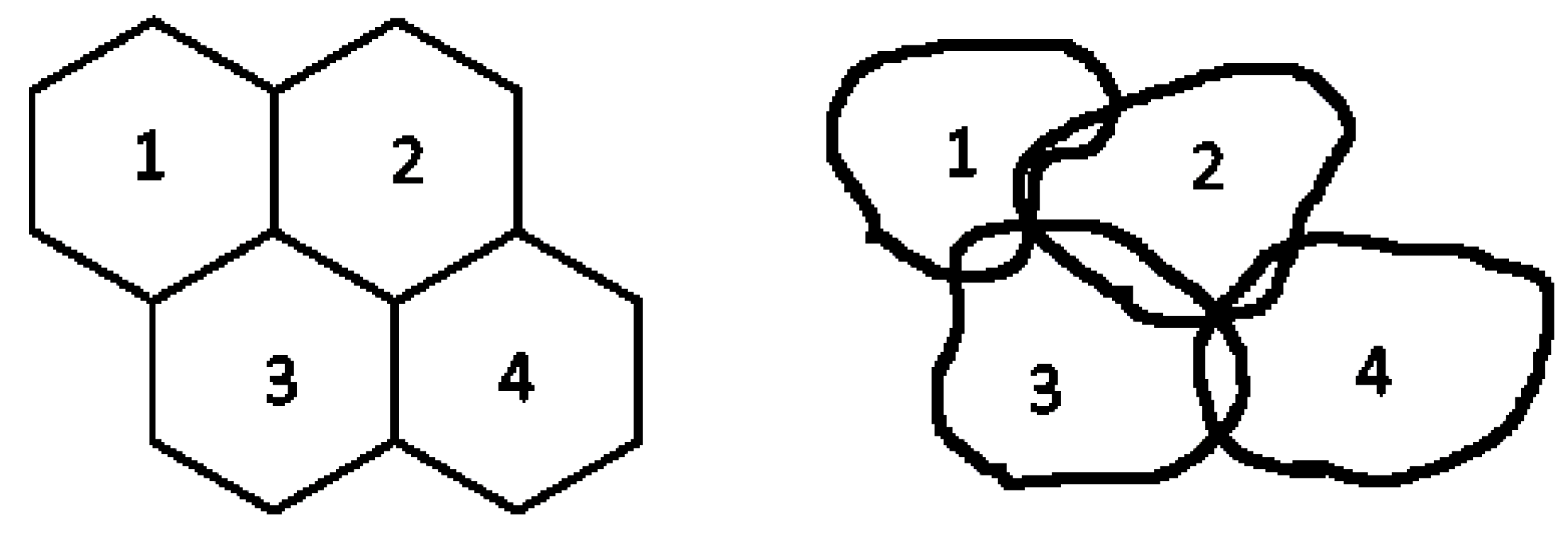
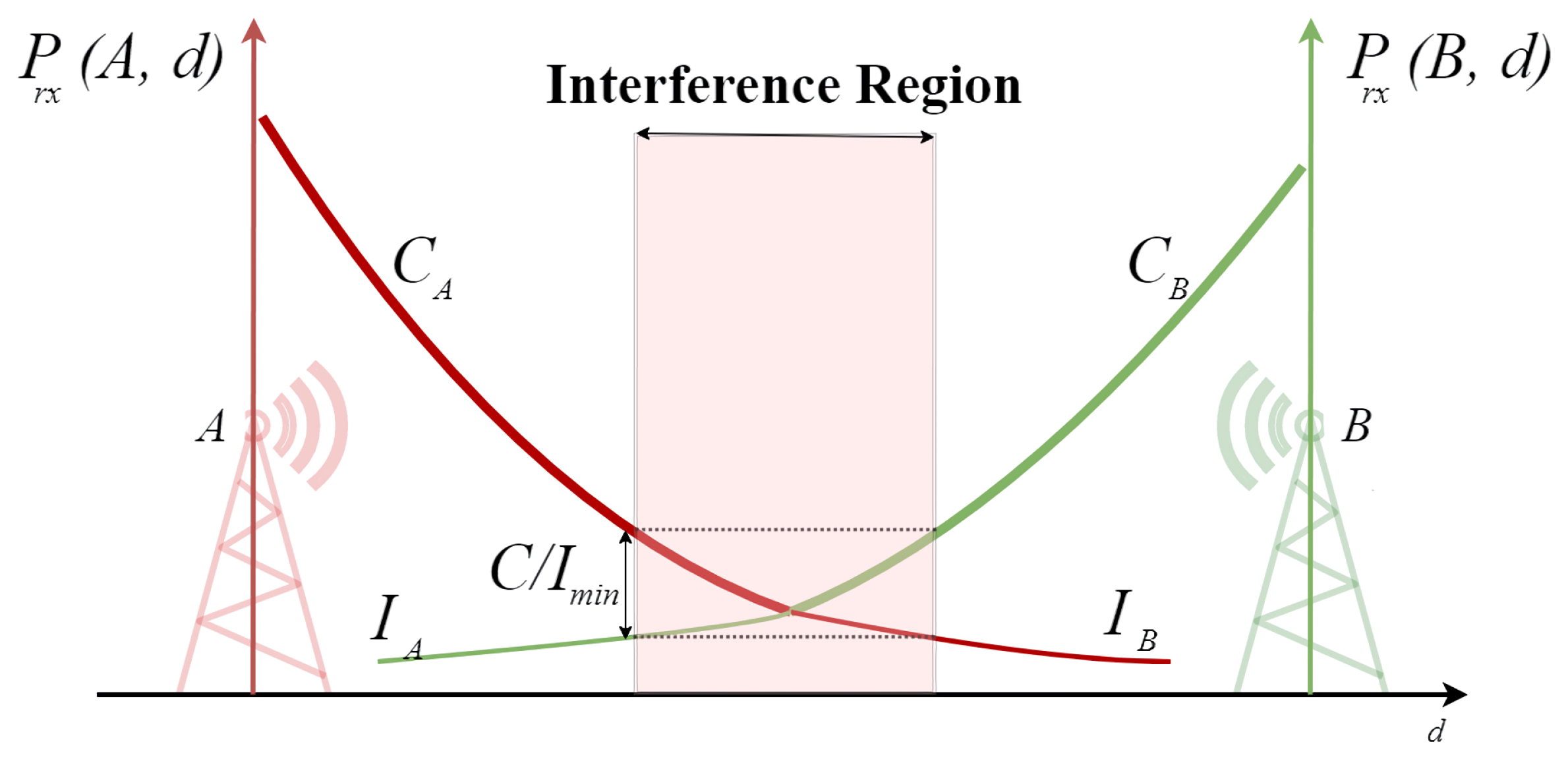
• Co-channel interference: The interference created from other cells with the same frequency. This is solved by spacing cells with the same frequency and splitting the cell in sectors (sectorization).
• Adjacent Interference: The interference coming from adjacent channels in adjacent cells. This is easily solved with quality filters and making sure there are sufficient differences between the frequencies used in those cells.
• Self interference: A consequence from a cell’s signal reflecting from obstacles (buildings, mountains, etc.). Solved by correctly splitting downlink and uplink frequencies.

There are multiple ways to allocate frequencies. The most used are either fixed frequency allocation, where frequency allocation respects a set of constraints as well as possible, and minimum span allocation, where allocation is done using the minimum amount of frequencies still respecting those constraints. But there are other “out of the box” solutions. In 2010, Chao et al. [7] proposed a new method of frequency planning using a cell’s latitude, longitude, and azimuth, and comparing them with that cell’s neighbors, thereby predicting which cells will interfere with each other. However, this process is still manual and requires human intervention.

2.2. Self-Organizing Networks

Usually, mobile network design requires three phases. First is network planning, taking in account certain aspects such as coverage, interference, quality of service, and frequency reusing. Second comes monitoring: using KPIs to evaluate the current state of the network. Those KPIs are analyzed in the final phase, optimization, changing parameters such as cell direction and intensity, antenna height, and radio parameters. This process its manual, expensive, and time consuming. In order to solve these problems, an automated technology named SON was designed in order to automatically plan, configure, manage, optimize, and heal mobile networks. This technology is characterized by a life cycle (Figure 2) composed of three phases:

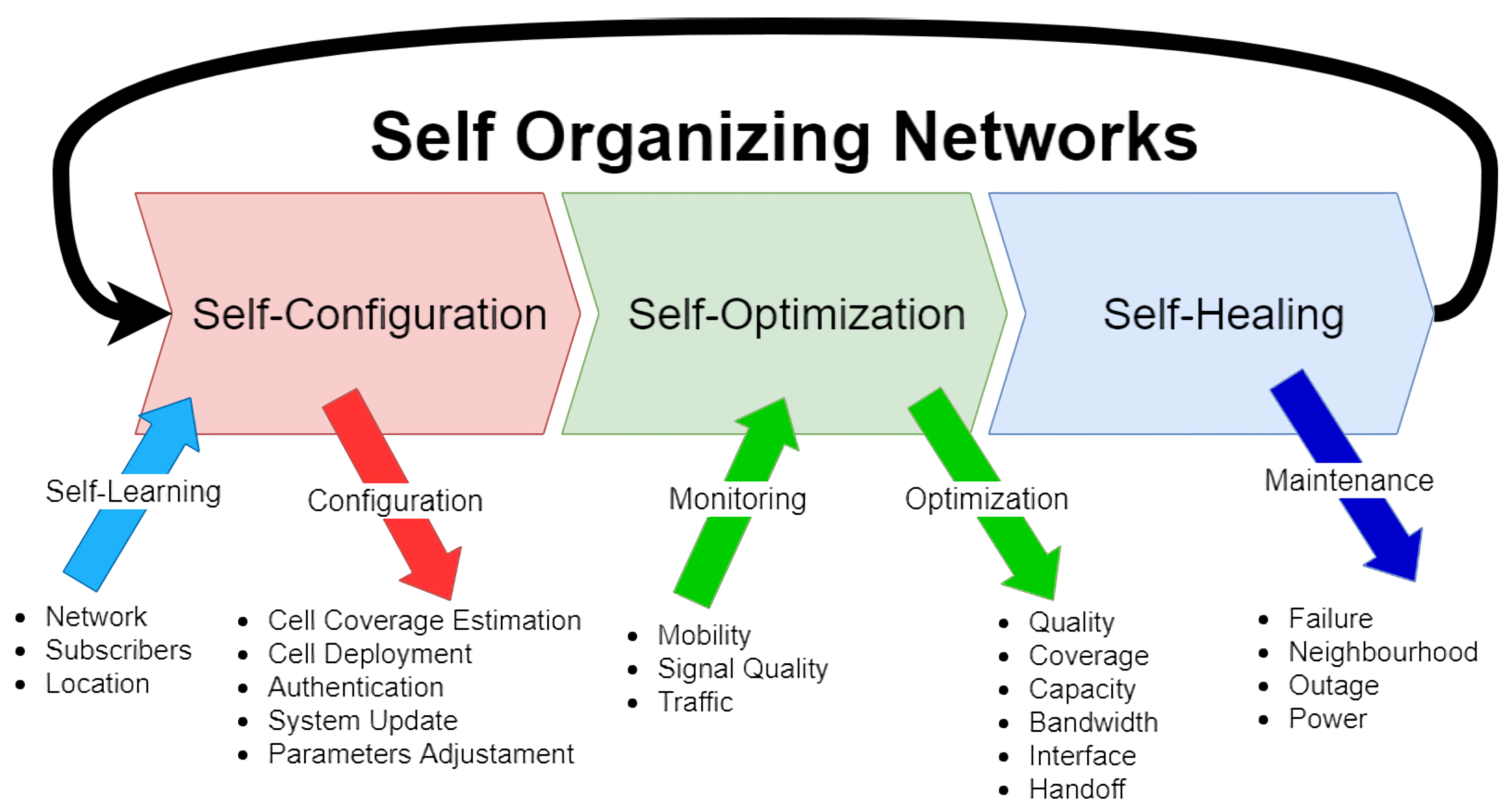
• Self-configuration: Following the idea of “plug and play,” this section is responsible for configuring a new node in a network, not only in connectivity but also for transferring the network parameters to that node.
• Self-optimization: Responsible for important factors in the network, such as topology, propagation, and interference (the one which is covered in this paper).
• Self-healing: In case some nodes fail. This section is responsible for warning the other nodes of that failure in order to reduce the impacts on the network’s services.

2.3. Cloud Services

Cloud services make it so that someone can connect and use applications based in the cloud. There are multiple advantages. Both users and companies can have access to complex applications without the need for specialized hardware/software. Not only that though, as users can usually access those applications on any device with internet access, which also means that all data are the same, regardless of that device. Finally, those applications are usually pay-per-use, avoiding expenses on unused services. Usually, the amount paid for these services is lower than the amount paid for management of dedicated hardware [8]. The clear definition and application of the service level agreement (SLA) are of paramount importance. Cloud-based solutions are only viable for a client if aspects such as quality and availability are defined between him and the service provider [9]. One example is Amazon Web Services (AWS), which contains services and applications in areas including databases, virtual servers, computation, machine learning, artificial intelligence, gaming, internet of things, and many others [10].

As illustrated in Figure 3, there are three standard types of service modules, each one defined by the National Institute of Standards and Technology (NIST) [11]:

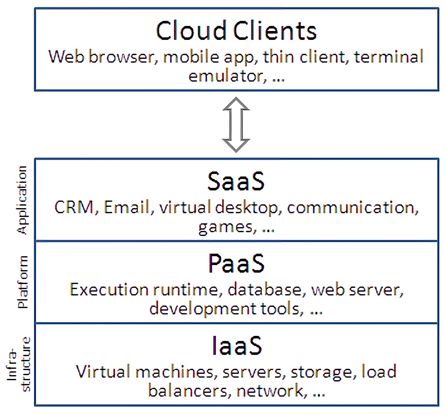
• Infrastructure as a service (IaaS): Where the consumer is able to deploy and run arbitrary software, which can include operating systems and applications. The consumer does not manage or control the underlying cloud infrastructure but has control over operating systems, storage, and deployed applications; and possibly limited control of select networking components (e.g., host firewalls).
• Platform as a service (PaaS): The capability provided to the consumer is to deploy onto the cloud infrastructure consumer-created or acquired applications created using programming languages, libraries, services, and tools supported by the provider. The consumer does not manage or control the underlying cloud infrastructure including network, servers, operating systems, or storage, but has control over the deployed applications and possibly configuration settings for the application-hosting environment.
• Software as a service (SaaS): The capability provided to the consumer is to use the provider’s applications running on a cloud infrastructure. The applications are accessible from various client devices through either a thin client interface, such as a web browser (e.g., web-based email), or a program interface. The consumer does not manage or control the underlying cloud infrastructure including network, servers, operating systems, storage, or even individual application capabilities, with the possible exception of limited user-specific application configuration settings.

Another service model is function as a service (FaaS), also associated with serverless computing [13]. Instead of using a continuously working virtual machine, FaaS enables the deployment of single functions which are only executed after a trigger or an event. This might be a better alternative for running code which does not have to execute multiple times or/and for a long time. One example of FaaS is AWS Lambda [14].

2.4. Metric SaaS and Other Commercial Tools

Metric SaaS is software as a service for commercial use, created and maintained by Multivision Lda. This service allows easy access of network data, reports, and issues, to everyone in a team. Network data, such as “RxLevel,” “Interference,” cell frequency, and many others, can not only be visualized on a map (Figure 4), but also imported to any system.

Metric already has integration for SON in both monitoring and maintenance. Our objective is to add the integration in optimization by automatically calculating interference and the best frequency allocation.

There are different commercial tools used in mobile network design. For example, WinProp is able to accurately simulate propagation data of cells in multiple environments, such as rural, urban, indoor, and underground [15]. However, it lacks other planning tools like neighbors lists.

Atoll is one of the most used by operators [16]. It runs as a local application with some installations opting for connectivity to external databases that are outside of the application scope license. The user needs, at least, an up-to-date machine with the minimum capacity to plan a set of cells in a reasonable amount of time. Although we do not have access to the application internals, its modus operandi suggests that it follows some type of simulated annealing implementation where time invested in computation translates into an improved frequency planning. This approach looks like a planning gamble and it would be interesting to see whether the product produces different results with different parameterization seeds running in multiple machines in parallel, but we pushed this type of analysis away for future benchmark work. Nevertheless, we acknowledge the strategic option, since with such limited resources and without the possibility of scaling the computation horizontally, it is a reasonable compromise.

Mentum Planet nowadays is part of the InfoVista tool panoply [17]. It does not suffer from the local limitations of a single machine, but it is still bound to an on-premises infrastructure that the user needs to setup up-front. It is possible to integrate multiple data sources, but Planet is basically a bunch of build-stitching tools and services that InfoVista acquired along its path to conquering a larger market share. The stitching of different technologies created a tool hard to use, one plagued with a licensing plan very hard to grasp even for the most basic usage. A user that only wants to evaluate the suite for frequency planning should accept a slow learning curve.

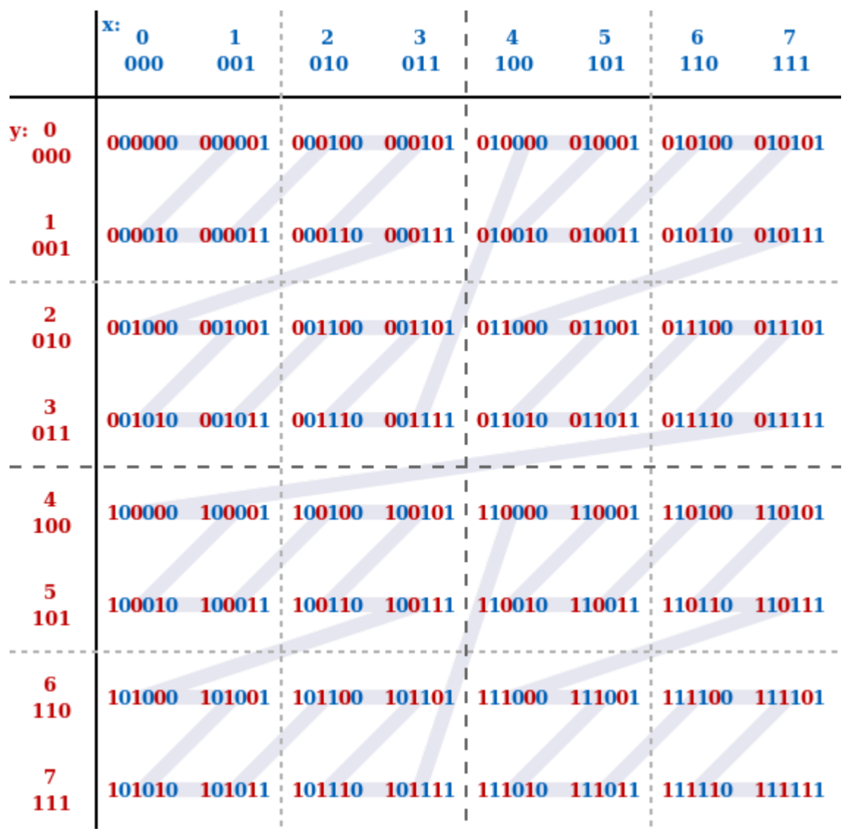
2.5. Z-Order Curve and Geohash

At a certain point in our implementation, we had to uniformly identify geographic areas around the world. Z-order curve is an algorithm which converts multidimensional data in unidimensional without losing original information. It was created and first used by Guy Macdonald Morton for file sequencing in 1966 [18]. Basically, the transformation is done by interleaving the binary representations of each coordinate, as illustrated in Figure 5. There are multiple applications of the Z-order curve, including linear algebra [19,20], texture mapping, image/video encoding, and quadtree generation [21].

Gustavo Niemeyer used this function on the invention of Geohash [22], a geographic encoder that transforms geographic coordinates in a unique hash representing them. Although, soon it was noticed that there were other applications for its use, as it began being used for unique identifiers and point data representations in databases, for example, in MongoDB [23]. The size of this hash defines its precision; the larger its size the better its precision (

Table 1. Geohash length and its precision with geographic coordinates.

Geohash Length	Cell Width [km]	Cell Height [km]
1	5000	5000
2	1250	625
3	156	156
4	39.1	19.5
5	4.89	4.89
6	1.22	0.61
7	0.153	0.153
8	0.0382	0.0191
9	0.00477	0.00477
10	0.00119	0.000595

).

There are some problems in the Geohash algorithm. Usually, one can use Geohash prefixes to find points in proximity with each other. The first problem is that, in edge case locations, those prefixes are not similar at all. For example, “s0000” and “kpbpb” are adjacent geohashes, but since they are in different halves of the world (north of the equator and south of the equator respectively), their prefixes are not similar. The second problem is the lack of linearity in the Geohash distance representation of our planet, since single degrees in latitude and longitude represent different distances. At the equator there is an error of 0.67%, at 30 degrees latitude there is an error of 14.89%, and at 60 degrees there is an error of 99.67%, tending to infinity the closer one goes to the poles. The source of this problem is not Geohash itself but the difficulty of converting coordinates on a sphere to a unidimensional value.

2.6. Linear Programming

Linear programming, or linear optimization, is a method whose objective is to find the best outcome of a mathematical model using linear constraints. Linear programming was already used in the past for channel allocation in large and cellular and radio networks [24]. Even though this is a powerful tool, learning linear programming is time consuming, especially for people with no programming/mathematical background.

There are multiple linear programming solvers available, although most of them are either paid or have proprietary licenses. We analyzed some Copyleft licensed software, including Coin-or linear programming (CLP), GNU Linear Programming Kit (GLPK), Cassowary constraint solver, Lp_Solve, and Qoca. Even though GLPK appeared to be one of the least efficient (especially when compared to commercial solvers) [25,26], it had the advantage of an already available layer for AWS Lambda [27].

There are also multiple input formats. For GLPK in particular, there are four:

• CPLEX-LP: Used in IBM ILOG CPLEX Optimization Studio, a commercially available optimization software package. More user-friendly than the others.
• MPS: Mathematical Programming System is a file format used in both linear programming and mixed integer programming problems. There are some limitations though; for example, numeric fields limited to 12 characters. Modern extensions of this format, without those limitations, are also accepted by GLPK.
• GLPK: A custom format, similar to DINAMICS format, a format created by the Center for Discrete Mathematics and Theoretical Computer Science;
• MathProg—High level modelling language. GLPK MathProg translator is not appropriate for large models, due to its taking a considerable amount of time with big problems. This happens because the translator is not able to recognize shortcuts on the optimization.

We ended up using the MathProg format, since the models are not that big and it is possible to structure it, cluing the solver in on optimization paths for faster optimization. In case someone finds a model to take a long optimization time, they can use GLPK to convert a MathProg format in any of the other formats. There are cases where converting first and optimizing later is more efficient.

2.7. Optimization Algorithm for Planning

Within frequency planning, the main goal is that the set of channels allocated to each cell minimizes interference. For a given geographic position, the carrier to interference ratio ($C/I$) measures the ratio between the cell’s signal power level and the sum of power levels of cells operating in the same frequency. A system is only capable of operating above a minimum value, $C/I_{min}$. An interference region, depicted in Figure 6, is characterized by $C/I$ levels below $C/I_{min}$, an area where communication is not possible in the evaluated frequency.

The proposed algorithm evaluates, for each unplanned cell c, the interference experienced when operating on each of the available BCCHs, the best server cell, $c_{f,b}$, shall correspond to the cell with strongest received signal level, $P_{rx}$. Remaining cells operating in f with signal present in pixel $\mathit{p}$ are the set of non-best server cells, $\pm c_{f,nb}$. Thus, a given covered pixel $\mathit{p}$ of c is labeled as interfered if $C/I$ is below $C/I_{min}$:

$$\frac{P_{rx}(\mathit{p},c_{f,b})}{{\sum }_{c_{f,n}\in {\mathit{c}}_{f,nb}}{P}_{rx}(\mathit{p},c_{f,nb})}<{(C/I)}_{min}$$

(1)

where $P_{rx}(\mathit{p},c_{f,b})$ (mW) is the received signal power level in pixel $\mathit{p}$ of best server cell $c_{f,b}$; $P_{rx}(\mathit{p},c_{f,nb})$ (mW) is the received signal power level in pixel $\mathit{p}$ of non-best server cell $c_{f,nb}$, belonging to ${\mathit{c}}_{f,nb}$ set; and ${(C/I)}_{min}$ is the minimum $C/I$ level that guarantees interference free communication. In GSM this value is typically taken as 9 dB.

For the unplanned cells set, $\mathit{c}$, and the set of sorted frequencies, $\mathit{f}$, $\mathit{D}$ matrix is built. It has dimension $dim\left(\mathit{c}\right)\times dim\left(\mathit{f}\right)$, having for each cell and frequency the number of pixels with interference; i.e., where condition (1) is observed. The objective is to minimize interference, given mathematically by:

$$min\sum _{c\in \mathit{c}}\sum _{f\in \mathit{f}}{\mathit{D}}_{cf}\times {\mathit{X}}_{cf}^T$$

(2)

where $\mathit{X}$ is a Boolean matrix with similar dimensions as $\mathit{D}$.

When various cells of different sites shall be planned, the amount of possible interference created by unplanned cells that share the coverage area is also minimized, in case these cells get the same BCCH:

$$min\forall f\in \mathit{f}and\forall c_1,c_2\in \mathit{c}:\left({\mathit{X}}_{c_{1}f}+{\mathit{X}}_{c_{2}f}\right)\times {\mathit{U}}_{c_1{c}_2}$$

(3)

where ${\mathit{U}}_{c_1{c}_2}$ is “1” if cells $c_1$ and $c_2$ interfere, and “0” otherwise. Two cells operating in the same BCCH interfere with each other when there are pixels covered by $c_1$ that are interfered by $c_2$. Nevertheless, this restriction shall be relaxed. In fact, the solution to this optimization problem may not be the best one or might even return a solution as impossible. Ideally, ${\mathit{U}}_{c_1{c}_2}$, would become an integer, representing the number of pixels in $c_1$ interfered by $c_2$. This minimization was originally a condition, but after some research on integer programming heuristics, we concluded that this way the optimization would be much faster (from hours to under a second, when optimizing 50 cells).

When planning frequencies, certain rules must be followed. These are expressed by a set of restrictions to the optimization problem. First, a single BCCH must be allocated to each unplanned cell:

$$\forall c\in \mathit{c}:\sum _{f\in \mathit{f}}{\mathit{X}}_{cf}=1$$

(4)

Secondly, cells of the same site $\mathit{s}$ (which may contain both planned and unplanned cells), cannot reuse the same BCCHs:

$$given\mathit{s},\forall f\in \mathit{f}:\sum _{c\in \mathit{s}}{\mathit{X}}_{cf}\le 1$$

(5)

Thirdly, the cells of $\mathit{s}$ cannot have adjacent frequencies. The sorted set of frequencies f is indexed, starting in index 0 and going until index $dim\left(\mathit{f}\right)$. This restriction can be expressed mathematically as follows:

$$\forall f_i,i\in [1,dim\left(\mathit{f}\right)]:\sum _{c\in \mathit{s}}\left({\mathit{X}}_{c{f}_{i-1}}-{\mathit{X}}_{c{f}_i}\right)\le 1$$

(6)

Regarding the planning of TCH, each cell has several TCH frequencies allocated. The same set of rules is applied to the optimization of TCH frequencies, with the exception that there needs to be at least a difference of two frequencies between TCHs of the cells of the same site:

$$\forall f_i,i\in [1,dim\left(\mathit{f}\right)]:\sum _{c\in \mathit{s}}\sum _{t\in {\mathit{t}}_c}\left({\mathit{X}}_{t{f}_{i-2}}-{\mathit{X}}_{t{f}_{i-1}}-{\mathit{X}}_{t{f}_i}\right)\le 1$$

(7)

where t_c identifies the set of available TCH channels of cell c.

2.8. Architecture

The architecture of our working pattern, as depicted in Figure 7 is basically a group of four modules linearly connected. The fact that it is cloud based not only allows us to communicate with the cellular network operation support system (OSS), but also, one can use each module individually for another reasons besides frequency planning.

Each module represents a processing service, while between each module will be a storage service, to save any inputs/outputs. We implemented four different processes:

• Cell coverage estimation module: Responsible for estimating a cell power around its location.
• Cell grid intersections module: Responsible for understanding which cell coverage intersects.
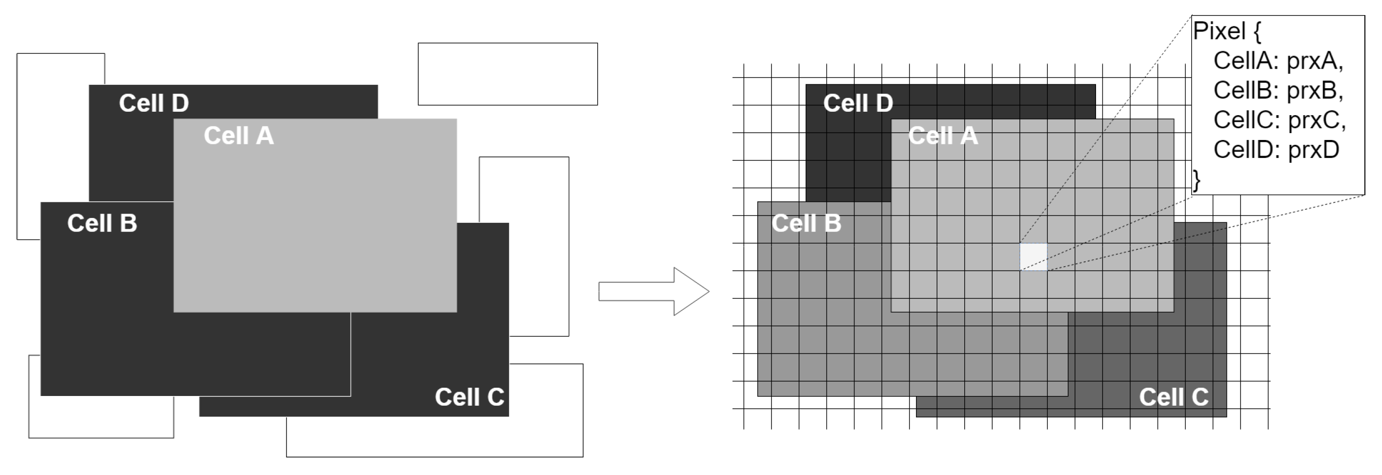
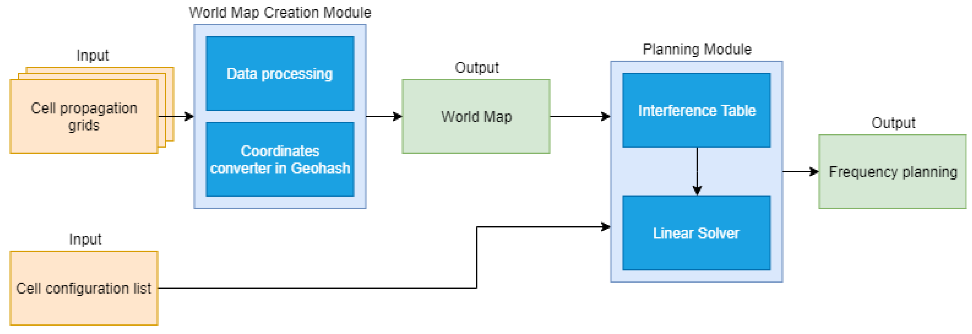
• World map creation module: Responsible for creating a world map, which is a data structure containing a set of pixels identified by their hashes—in this case, Geohashes. Each pixel will have an undefined number of pairs of cell/power.
• Planning module: Responsible for applying a linear optimization and its defined rules to the data generated by the previous modules.

The four steps of the pattern are detailed in the next sections.

2.9. Cell Coverage Estimation Module

An algorithm that was created by Fernandes et al. [28]. It uses drive tests (DT)—tests done, usually in a vehicle, to obtain coverage data in an area and evaluate its quality—to calibrate a standard propagation model (SPM) [29]. This module, given information recovered from Metris SaaS, such as an antenna diagram, cell information, DTs, and altimetry data extracted from OpenTopography, outputs a propagation grid with power estimation on areas covered by the cell, as depicted in Figure 8.

2.10. Cell Grid Intersection Module

A simple module computes a list of cells whose coverage intersects with the one being computed, as depicted in Figure 9. It takes on the pessimistic perspective, by drawing an imaginary rectangle where the coverage fits in and checks whether those rectangle borders intersect with any neighboring ones. Depending on the lists’ sizes, it has two operational modes: computing the lists using a quad tree to make small lists and computing the potential intersection between all of them for larger lists, since the construction of a quad tree is computationally heavy.

All data from this and the previous module were compiled and processed in the World map creation module (Figure 10).

2.11. World Map Creation Module

It is common sense that a computer works better with discrete data, rather than continuous data. Knowing this, it is important to find a way to uniformly and coherently split the world into small areas, in order for us to be able to compare cell powers in mutual areas and check for interference, as illustrated in Figure 9.

As explained in Section 2.5, Geohash covered our requirements; even though there is an increasing error the closer we go to the poles, this is not significant, since we only care that the area between different cells that are both in the exact same space and have the exact same size.

This module generates a world map. A world map is a data structure containing pixels representing the area covered by our problem (area covered by all cells we are trying to plan). We compute each propagation grid mentioned in Section 2.9 of each cell participating in our problem, all of which were identified by the lists created in Section 2.10.

The module outputs a Tab-Separated Values (TSV) file representing a map, where each line is identified by a Geohash, followed by pairs of cell/power. With this we can easily identify which cells are in a certain area and their corresponding powers. We tried other file types and structures, but upon some testing, we noticed that all the others would either take up more space and/or were too slow to realistically process.

2.12. Planning Module

Iterating trough the world map, pixel by pixel, we calculate whether the $C/I$ is enough to make telecommunication services unusable in that area. At the same time, a table with unplanned cells as rows and frequencies as columns is populated with the size of the area interfered with. Another table is also populated to check interference between unplanned cells if they end up having the same frequency. These tables, in conjunction with the equations described in Section 2.7, are sent to the optimizer, which returns the best solution to the given problem.

2.13. Technology Used

This program is part of the automatic GSM frequency planning package Cloud-based Pixelized Site Planning (CPSP), within the Metric SaaS ecosystem [4]. It was written completely in Java 8 [30] and compiled by Maven [31], and each module is packaged into executable JARs which are hosted in AWS Lambdas, a serverless computing platform provided by Amazon Web Services (FaaS) [10].

We discussed the possibility of hosting the executables in another service call Elastic Computer Cloud (EC2), an infrastructure as a service, but we came to the conclusion that each of our modules was not supposed to run continuously; they were supposed to only run when needed, either because of a trigger or a call. If we used EC2 we would be paying continuously for the service, even if we were not using it—the opposite to AWS Lambda. Using AWS cloud services also allowed to integrate our implementation, described in Section 2.8, in Metric SaaS. Currently, a user requests to plan GSM frequencies in its interface.

All Lambda inputs/outputs are streamed/saved in S3 buckets, a storage service (PaaS).

Finally, as explained in Section 2.6, we use GLPK solver (GLPSOL), to solve models in MathProg format.

2.14. Implementation of the Work Pattern

In Figure 11 is detailed the pattern that implements the proposed framework using AWS Services. It receives information from the OSS and returns a set of frequency allocations to each cell we are trying to plan. We can also see in the same figure that between each Lambda, all processed data are saved in S3 buckets whose IDs depend on the client information. This data include but are not limited to: propagation grids, intersection files, world maps, interference matrixes, cell configurations, and other client data.

Each lambda receives a JSON file as input. In this case, the file must have the names of the cells we want to plan, the frequency to which they must be planned as designed by the International Telecommunication Union (ITU) in GSM operations, and client information for file access, which is automatically input based on the login session.

There are some restrictions about each individual lambda one needs to take into account:

• Maximum memory allocated is 3008 MB;
• Timeout of 900 s (15 min);
• Virtual storage is limited to 500 MB.

This is important because the world map can take a considerable amount of space; therefore, the implementation of streaming when reading a world map is a must. The same happens when uploading a file to a bucket, since the file must first be created in Lambda’s temporary storage and only then uploaded. Problems might appear when planning a large problem, where the optimization can take a long time.

Another possible problem was the fact that S3 buckets have a limit of 5 TB per object, but that does not compare to the 500 MB of Lambda virtual storage, meaning that it can be ignored. There is also a limit of 100 buckets (1000 with premium) per account, which again is not a problem, since we would need five at max.

In Figure 11 we have the following AWS lambdas:

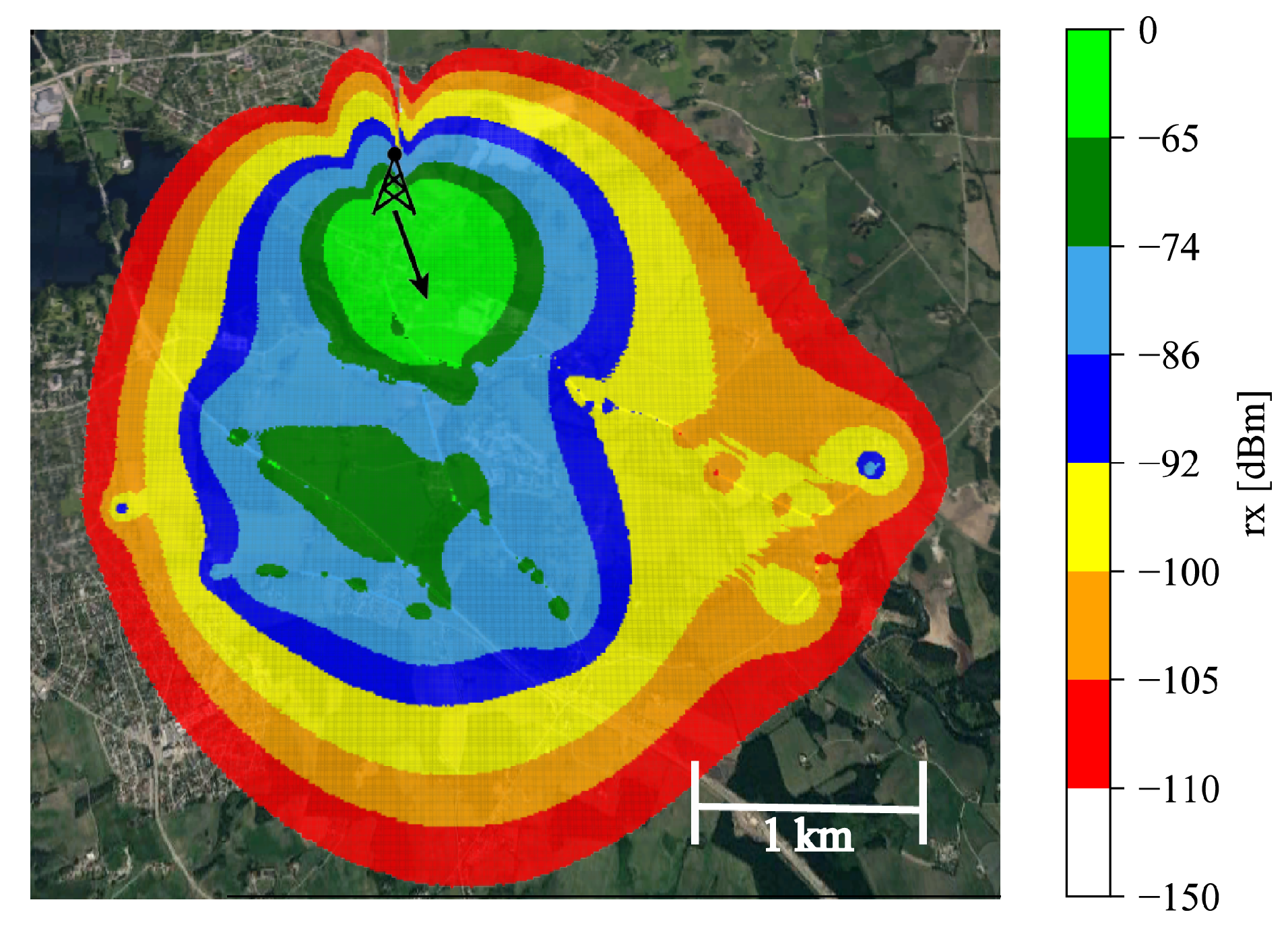
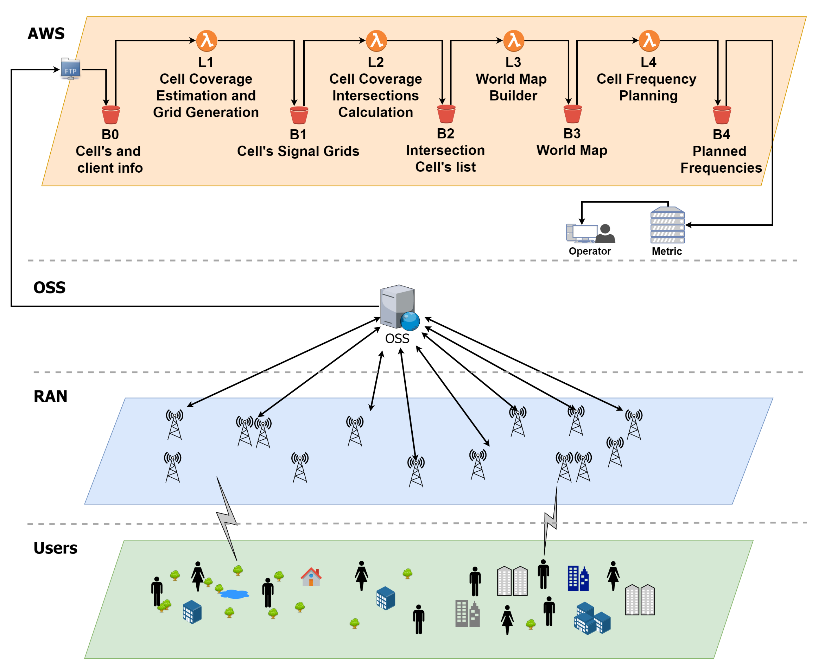
• Cell coverage estimation and grid generationAWS Lambda (L1): Using client information imported from a S3 bucket (B0), this lambda creates a pixelized grid with coverage information around an antenna. This coverage is calculated using propagation modules, drive tests, and other cell parameters, such as elevation, azimuth, and tilt [32]. Those grids will be saved in an S3 bucket (B1);
• IntersectionsAWS Lambda (L2): Using a metadata file imported from B1, L2 compiles that data verifying which cells’ coverage intersects, by getting two opposite max distance corners. Finally, it outputs that data in a CSV file to B2.
• World MapAWS Lambda (L3): This lambda is responsible for creating a TSV file with Geohash keys and pairs of cell/power, which we call a “World Map.” Both those grids and the map must have the same Geohash precision (BitSet size) in order to avoid scale/localization incoherence. First, we use the intersection files from B2 to iterate trough the set of cells that we are trying to plan and find the corresponding intersection files. A new set of cells is created that includes all the cells that intersect the ones we are trying to plan. We use the propagation grids of those cells (imported from B1) to compile and create a world map containing all those cells. At first, we tried to use a Json file, but its size ended up being too large to read in a reasonable amount of time.
• PlanningAWS Lambda (L4): First, we count both the amount of interference in the world map, and the amount of possible interference in the case in which the unplanned cells end up with the same frequency. Reminder that interference is defined by Equation (1). All data are written and sent to the GLPSOl module from GLPK library [33], a linear solver, in a “mathProg” file. In that file is also written the solver’s objective (Equation (2)) and all rules (Equations (3)–(7)). The outputted solution should have multiple $x[c,f]$ where x equals either 1 or 0. In case of the former, it means that frequency f should be attributed to cell c. That data are exported using a regex—“$\backslash [$(\d+),(\w*)$\backslash ]$\s?\W*1”—computed, and sent back to the user.

All S3 file requests are made by reading the stream from the online connection to an S3 bucket, without the need to save the information in temporary files and avoiding the possible problem of using more than the available 500 MB of temporary storage.

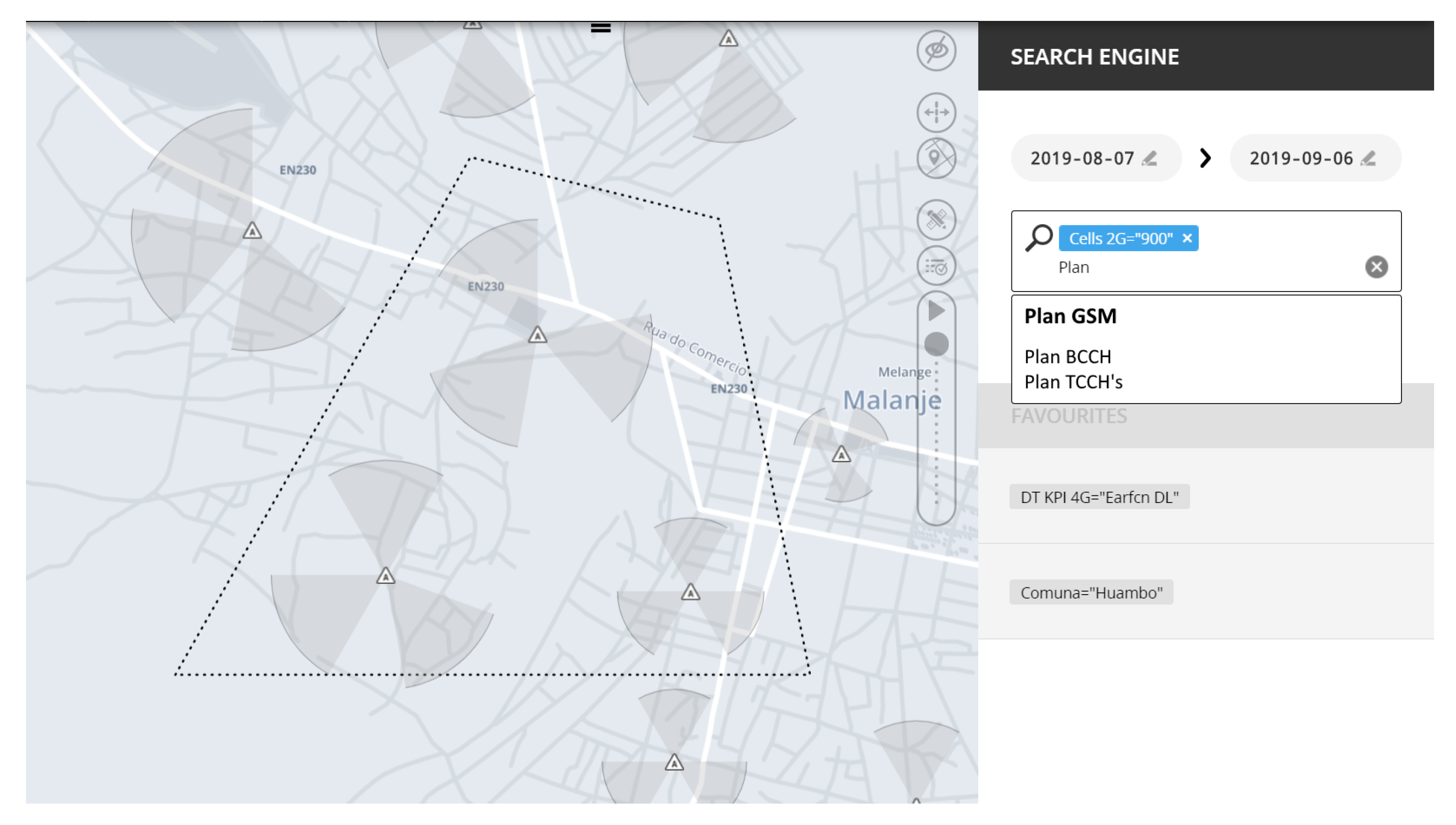
2.15. Integration in Metric

The pattern was integrated in Metric SaaS, currently available in its current version. The user starts by selecting an area of sites to plan and then asking for a planning of those sites (Figure 12). The system then sends a request to AWS Web services, which after processing the data returns the best planning to that area.

3. Experiment, Results, and Discussion

In the next sections, we will set the evaluation scenario and discuss both the experiments done and their results.

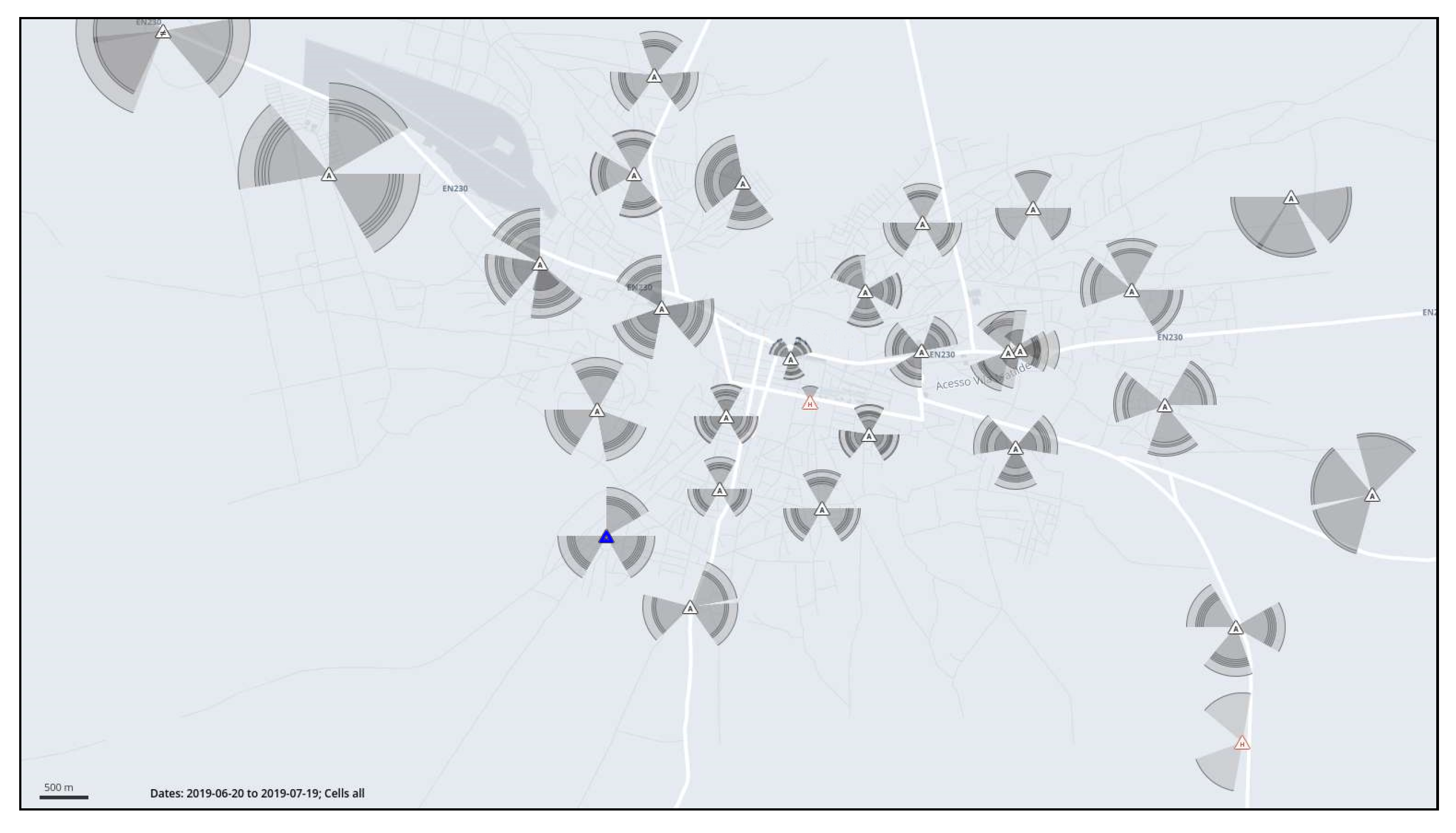
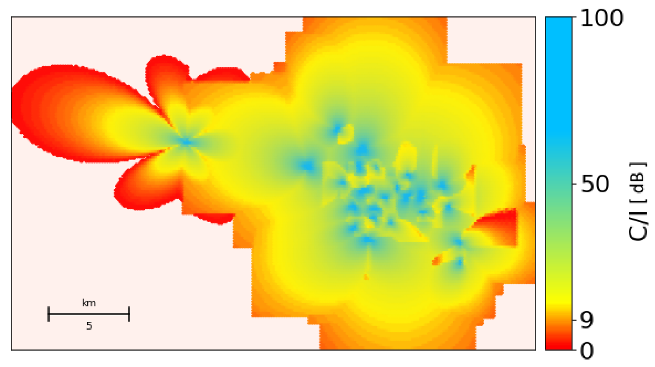
3.1. Evaluation Scenario

A scenario for evaluation is proposed, consisting of real operator data from a GSM network deployment, corresponding to an urban area of 2422 km² with around 570,000 inhabitants. Figure 13 represents the reference scenario with the existing deployment. This deployment congregates 23 sites with a total of 70 cells. The city center is intensely covered with cells, while for the surrounding rural areas cells are only present along streets. The BCCHs used by the operator are in the 900 MHz band, with channels between 63 and 88, while for the 1800 MHz band, channels range between 733 and 769. The TCH channels for 900 MHz range between 89 and 124, while for 1800 MHz they are between 770 and 824.

This scenario was split into two reference scenarios. First, a single site scenario of three cells was manually planned. The site is colored blue in Figure 13. Second was the whole scenario of 70 cells operating in specific channels.

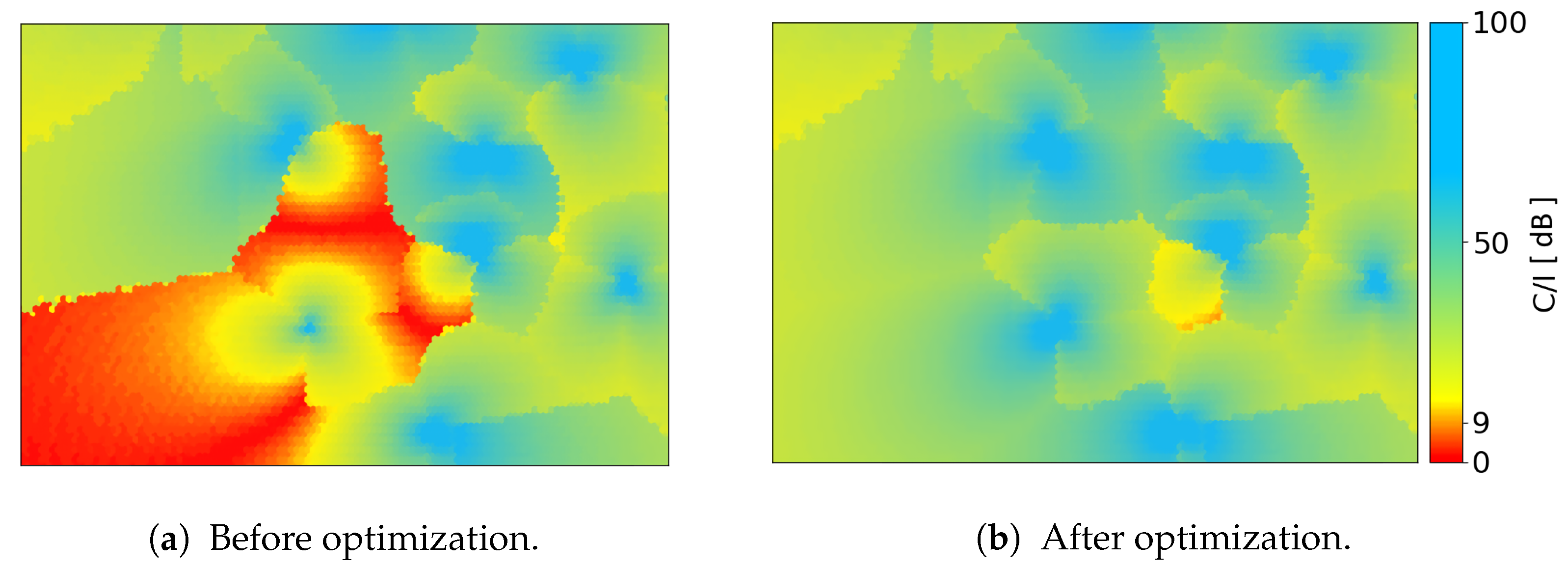
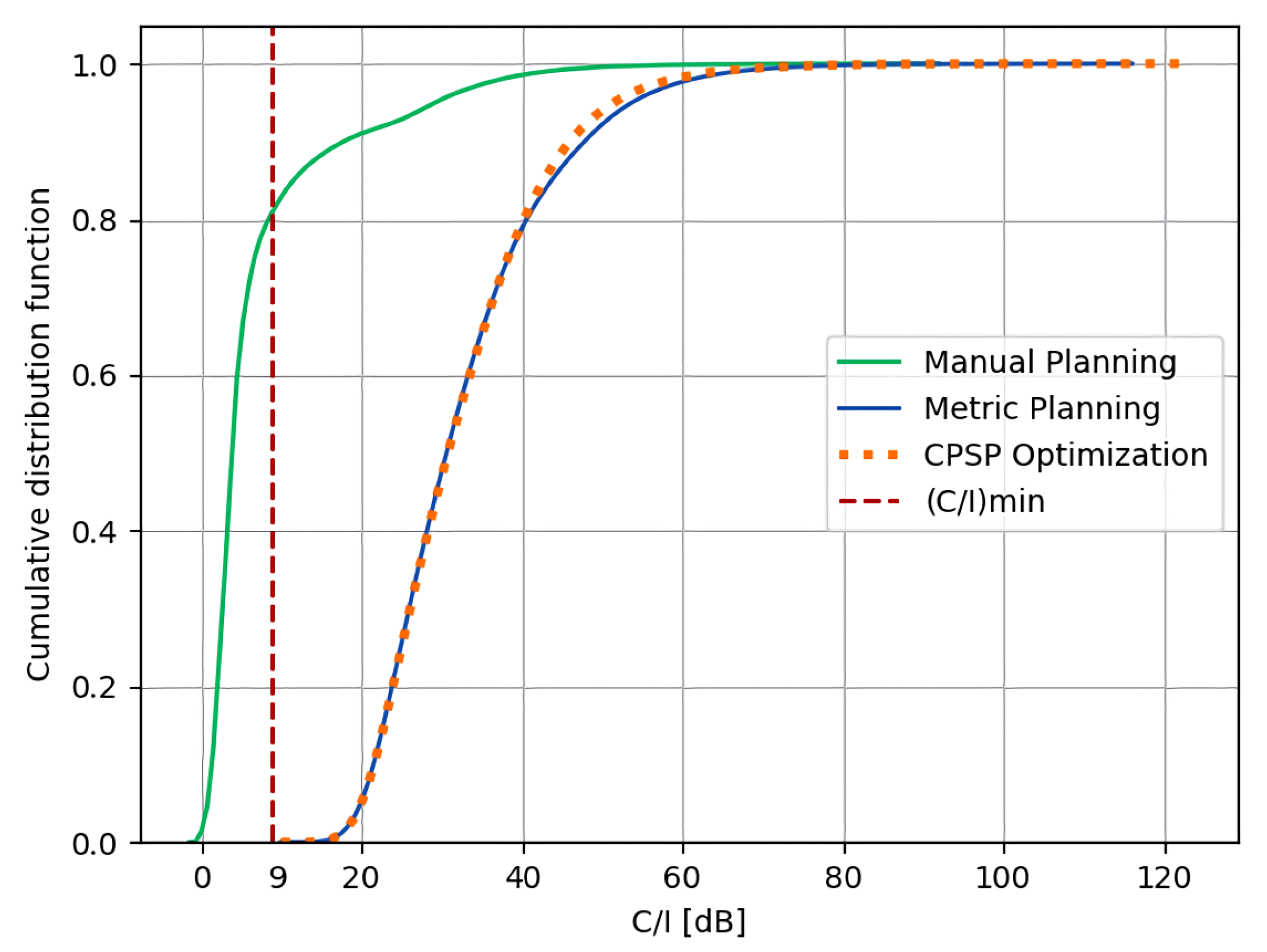
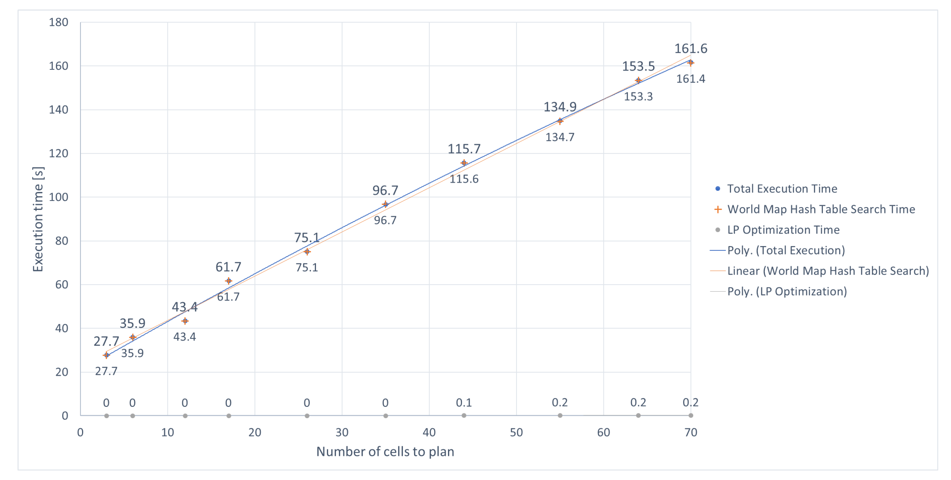
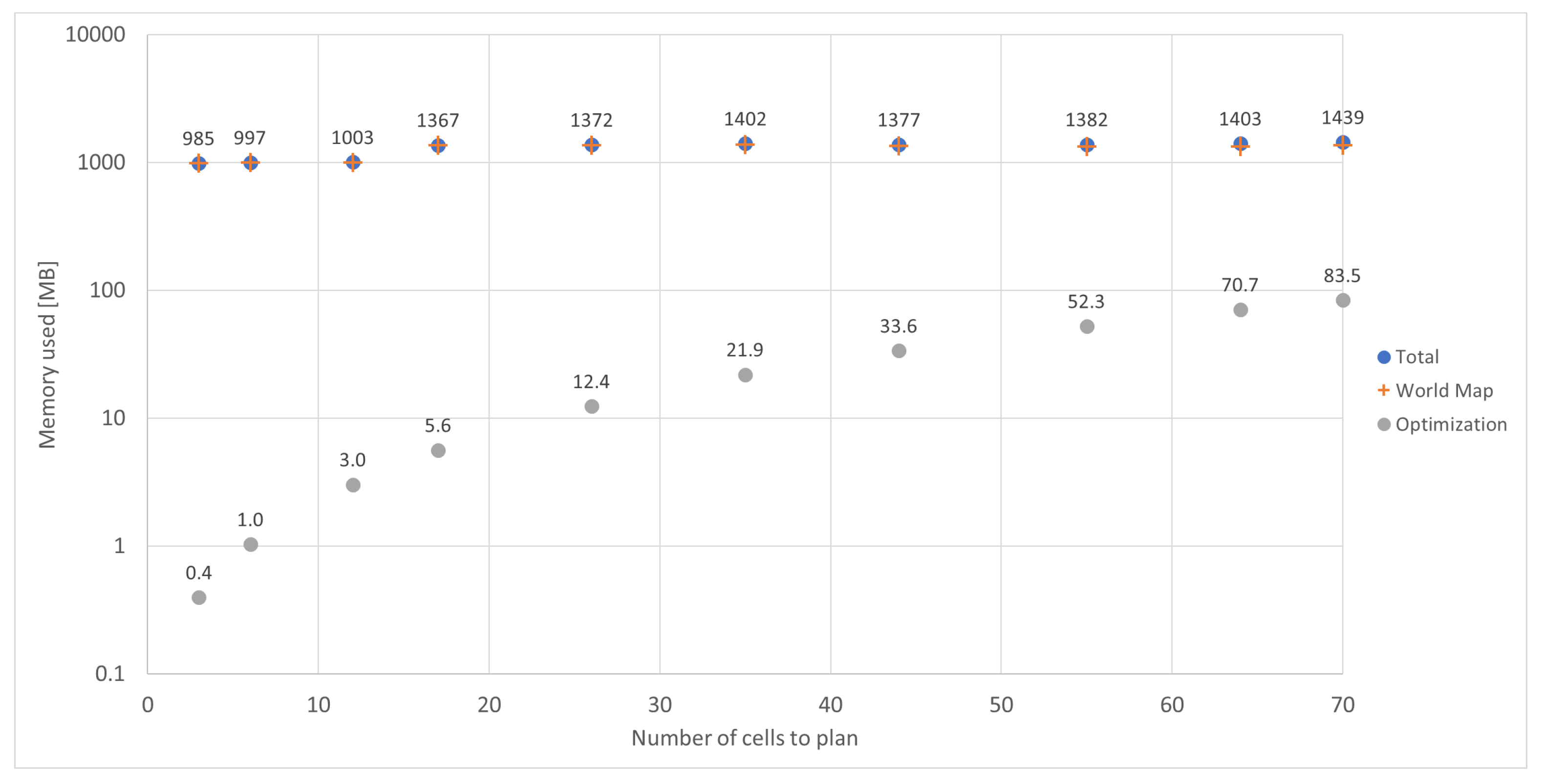
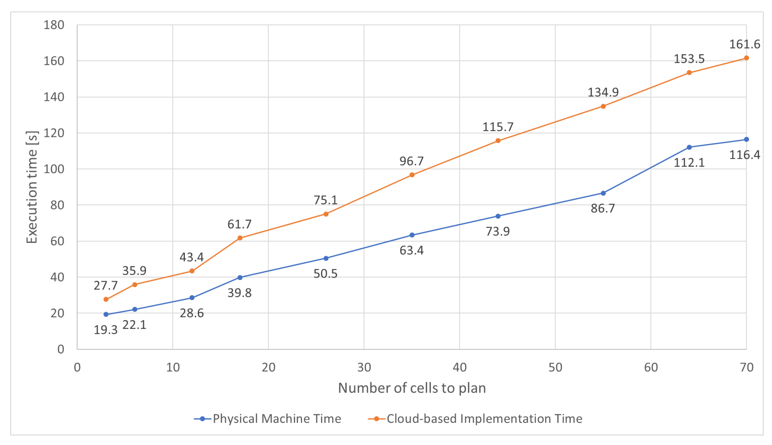
3.2. Implementation Results and Discussion

After some initial simple assessment tests, the model was applied to our evaluation scenario. Initially, we tested the planning of the site with three cells. We generated with the $C/I$ of each pixel covered by that site: one with the original operator frequency planning, before optimization (Figure 14a) and after the CPSP planning (Figure 14b). The implementation in Metric was also used to assess the results of the proposed methodology. It runs in a physical machine while the proposed CPSP is cloud-based. Additionally, in terms of propagation, it uses the Okumura–Hata model to estimate receive power levels, requiring larger computation resources, as will be shown. It splits the “world” using angles and distances, creating a non-uniform grid. A strong limitation of the Metric algorithm is that its constraints only apply when planning cells from the same site. In this sense, planning a network with multiple sites can only be done sequentially, resulting in a non-optimal global solution.

An empirical cumulative distribution function is generated, as represented in Figure 15, in order to compare network quality. Keep in mind that this distribution does not take in account pixels where the power of the most potent cell is not enough to enable connectivity, as the quality of the planning of the frequencies is not affected by it. Both CPSP and Metric plannings, even though they had different frequencies allocated, achieved similar network quality, as can be verified in Figure 15, and in an identical heatmap, Figure 14b. Before optimization, the manual planning depicted in Figure 14a achieved 83.7% of the coverage area and below ${(C/I)}_{min}$ (9 dB). The bad quality of the area is visible by the average $C/I$ of 7 dB. After planning, we can observe in Figure 15 that 99.9% of the coverage area is above 15 dB (6 dB higher than ${(C/I)}_{min}$), enabling communication with excellent quality.

For the scenario in under analysis, the proposed CPSP planning algorithm is compared to the one of the Metric tool. Even though both achieve similar results, as is visible in Figure 15, their performances are different, in terms of execution time and memory usage efficiency, as depicted in Figure 16. For planning three cells, the proposed algorithm used up 985 MB of memory, taking 27.7 s to execute, an improvement compared to the 4096 MBs used and 329.2 s from the already implemented one. The proposed algorithm is almost 12 times faster and four times less memory consuming. These results exclude the time and memory used to calculate the pre-processed propagation grids, which are pre-processed and available by Metric SaaS. Both the memory and time reduction can be explained by the more uniform world division and by the fact that the world map is generated once instead of in multiple individual generations for each cell.

We then applied the algorithm to the whole scenario of 70 cells, in order to check how the pattern would behave when planning multiple sites, taking 161.6 s and using 1439 MB of memory (Figure 17. We cannot compare it to metric since it can only plan a site at the time, but it could plan each site individually, one by one, taking 70 times 329 s (23,044 s). This approach has another major problem. The obtained solution might not be the best one because of the planning order.

The proposed procedure is composed of searches in the world map, a hashtable and linear optimization. For the next results, “World map” covers everything from reading the required files for generating the world map, to the process of sending the problem to optimization. The complexity of search on a hashtable is $O\left(n\right)$, and the LP used has a time complexity of $poly\left(n\right)$ [34]. Therefore, the proposed procedure is also $poly\left(n\right)$. To illustrate and confirm that, we show in Figure 18 that, even though it looks linear, the best approximation for the time complexity is polynomial. The reason for this illusion is because the polynomial trendline from LP optimization does not have much of an effect when planning small numbers of cells. The small variance in the time complexity is due to the time consumed while reading and writing on hard memory.

For space complexity, depicted in Figure 19 using a logarithmic scale, even though linear optimization shows a space complexity of $poly\left(n\right)$, the space occupied by it is not significant when compared with the memory used by the world map creation module. Additionally, we cannot calculate space complexity for that module, since it depends more on a cell’s location than the map itself. The space occupied by a world map of three cells close to each other will be lower than the one of there cells far from each other, because there is more area to cover. This can be noticed in Figure 19, where there is a big memory difference between 12 and 17 cells.

We also compared execution times, of our working pattern, in both a physical machine and the cloud implementation (Figure 20). The physical machine was slightly faster when planning. This discrepancy might be explained by the fact that the cloud-based implementation loses some time in the process of downloading/uploading a file (this includes opening and closing a connection) to the S3 service.

4. Conclusions

We proposed a novel way of automatically planning cellular networks supported by linear programming and cloud computing and applied a test case to the GSM protocol. It was implemented with the help of cloud-services, easing up our process of joining each module and both speeding up execution time and lessening the amount of resources used.

For a realistic scenario with a problematic site, where 83.7% of the serving area had interference, the proposed planning algorithm was capable of removing interference, guaranteeing excellent conditions for communication in the whole serving area. This process was 12 times faster and used four times less space than a planning tool running in a physical machine (which can only plan and optimize one site). Additionally, both time and space complexity were discussed after planning the whole scenario of 70 cells; we noticed that optimizing larger networks might take an unrealistic amount of time.

Results show that the cloud-based implementation ends up being slightly slower than a physical implementation. However, there are still noticeable advantages to using cloud services, such as the pay-per-use approach, the non-necessity of buying specific hardware, and the fact that other features can use your modules by simply triggering them.

For future work, we propose an extension of this work pattern to other network technologies, including UMTS and LTE, and even the modern 5G. We also propose an evaluation of the working pattern using other linear programming solvers that might simplify or speed up the process. Finally, investigating a way of splitting the world map into smaller problems and sending them away for optimization, might prove worthwhile to larger scenarios.

References

1. Ericsson. Ericsson Mobility Report November 2019; Technical Report; Ericsson: Stockholm, Sweden, 2019. [Google Scholar]
2. Mishra, A.R. Advanced Cellular Network Planning and Optimisation: 2G/2.5G/3G—Evolution to 4G; John Wiley: Hoboken, NJ, USA, 2007; p. 521. [Google Scholar]
3. Huurdeman, A.A. The Worldwide History of Telecommunications; John Wiley & Sons, Inc.: Hoboken, NJ, USA, 2003. [Google Scholar] [CrossRef]
4. Multivision. Metric Software-as-a-Service; Multivision: Lisbon, Portugal, 2019. [Google Scholar]
5. Godinho, A.; Fernandes, D.; Clemente, D.; Soares, G.; Sebastião, P.; Ferreira, L. Cloud-based Cellular Network Planning System: Proof-of-Concept Implementation for GSM in AWS. In Proceedings of the 22nd International Symposium on Wireless Personal Multimedia Communications, Lisbon, Portugal, 24–27 November 2019. [Google Scholar]
6. Freeman, R.L. Fundamentals of Telecommunications, 2nd ed.; John Wiley & Sons, Inc.: Hoboken, NJ, USA, 2005. [Google Scholar]
7. Su, C.; Lan, L.; Yu, C.; Gou, X.; Zhang, X. A new method of frequency planning for new cells in GSM. In Proceedings of the 2010 2nd Conference on Environmental Science and Information Application Technology, ESIAT 2010, Wuhan, China, 17–18 July 2010; Volume 3, pp. 420–423. [Google Scholar] [CrossRef]
8. Avram, M. Advantages and Challenges of Adopting Cloud Computing from an Enterprise Perspective. Procedia Technol. 2014, 12, 529–534. [Google Scholar] [CrossRef] [Green Version]
9. Ghani, A.; Badshah, A.; Shamshirband, S.; Aceto, G.; Pescape, A. Performance-based Service LevelAgreement in Cloud Computing to OptimizePenalties and Revenue. IET Commun. 2020. [Google Scholar] [CrossRef]
10. Amazon. Amazon Web Services; Amazon: Seattle, WA, USA, 2019. [Google Scholar]
11. Mell, P.M.; Grance, T. The NIST Definition of Cloud Computing. Recommendations of the National Institute of Standards and Technology; Technical Report; National Institute of Standards and Technology: Gaithersburg, MD, USA, 2011. [Google Scholar] [CrossRef]
12. Uenlue, M. Amazon Business Model: Amazon Web Services; Innovation Tactics: Sydney, Australia, 2018. [Google Scholar]
13. Roberts, M. Serverless Architectures. Martinfowler.Com. 2016. Available online: https://martinfowler.com/articles/serverless.html (accessed on 4 April 2020).
14. AWS. AWS Lambda—Serverless Compute—Amazon Web Services; AWS: Seattle, WA, USA, 2018. [Google Scholar]
15. Altair. WinProp Software for Wave Propagation and Radio Planning. Available online: https://altairhyperworks.com/product/Feko/WinProp-Propagation-Modeling (accessed on 4 April 2020).
16. Forsk. Atoll Radio Planning Software Overview; Forsk: Toulouse, France, 2020. [Google Scholar]
17. Infovista. Mentum Planet 5.7 Streamlines Network Planning, Provides Immediate Gains for Mobile Operators; Infovista: Paris, France, 2013. [Google Scholar]
18. Morton, G.M. A Computer Oriented Geodetic Data Base and A New Technique in File Sequencing; Technical Report; IBM Ltd: Ottawa, ON, Canada, 1966. [Google Scholar]
19. Gilbert, J.R.; Leiserson, C.E.; Street, C. Parallel Sparse Matrix-Vector and Matrix-Transpose-Vector Multiplication Using Compressed Sparse Blocks Categories and Subject Descriptors. In Proceedings of the Twenty-First Annual Symposium on PARALLELISM in Algorithms and Architectures, Calgary, AB, Canada, 11–13 August 2009. [Google Scholar]
20. Valsalam, V.; Skjellum, A. A framework for high-performance matrix multiplication based on hierarchical abstractions, algorithms and optimized low-level kernels. Concurr. Comput. Pract. Exp. 2002, 14, 805–839. [Google Scholar] [CrossRef]
21. Bern, M.; Eppslein, D.; Teng, S.H. Parallel construction of quadtrees and quality triangulations. Lect. Notes Comput. Sci. Incl. Subser. Lect. Notes Artif. Intell. Lect. Notes Bioinform. 1993, 709, 188–199. [Google Scholar]
22. Niemeyer, G. Geohash| Labix Blog. Available online: https://web.archive.org/web/20080305223755/http://blog.labix.org:80/#post-85 (accessed on 21 June 2019).
23. MongoDB. MongoDB Manual—2d Index Internals; MongoDB: New York, MY, USA, 2019. [Google Scholar]
24. Hellebrandt, M.; Lambrecht, F.; Mathar, R.; Niessen, T.; Starke, R. Frequency allocation and linear programming. In Proceedings of the IEEE VTS 50th Vehicular Technology Conference, VTC 1999-Fall, Amsterdam, The Netherlands, 19–22 September 1999; Volume 1, pp. 617–621. [Google Scholar]
25. Gearhart, J.L.; Adair, K.L.; Detry, R.J.; Durfee, J.D.; Katherine, A.; Martin, N. Comparison of Open-Source Programming Solvers Linear; Technical Report; Sandia National Laboratories: Albuquerque, NM, USA, 2013. [Google Scholar]
26. Meindl, B.; Templ, M. Analysis of Commercial and Free and Open Source Solvers for Linear Optimization Problems; Technical Report 1; Institut, F., Statistik, U., Eds.; Wahrscheinlichkeitstheorie: Wien, Austria, 2012. [Google Scholar]
27. Tempusenergy. GitHub—Tempusenergy/glpk-Lambda-layer: Use an LP Solver in Your AWS Lambda Functions. Available online: https://github.com/tempusenergy/glpk-lambda-layer (accessed on 21 January 2020).
28. Fernandes, D.; Ferreira, L.S.; Nozari, M.; Sebastiao, P.; Cercas, F.; Dinis, R. Combining Drive Tests and Automatically Tuned Propagation Models in the Construction of Path Loss Grids. In Proceedings of the IEEE International Symposium on Personal, Indoor and Mobile Radio Communications (PIMRC), Bologna, Italy, 9–12 September 2018; pp. 1161–1162. [Google Scholar] [CrossRef]
29. Forsk. Atoll 3.3.0 Technical Reference Guide for Radio Networks; Technical Report; Forsk: Blagnac, France, 1997. [Google Scholar]
30. Java. Java | Oracle; Java: Redwood City, CF, USA, 2019. [Google Scholar]
31. The Apache Software Foundation. Maven—Welcome to Apache Maven; The Apache Software Foundation: Forest Hill, MD, USA, 2016. [Google Scholar]
32. Fernandes, D.; Ferreira, S.; Soares, G.; Sebasti, P.; Cercas, F.; Dinis, R.; Clemente, D.; Cortes, R. Combining Measurements and Propagation Models for Estimation of Coverage in Wireless Networks. In Proceedings of the 2019 IEEE 90th Vehicular Technology Conference (VTC-Fall), Honolulu, HI, USA, 22–25 September 2019. [Google Scholar]
33. Makhorin, A.M.A.I. GLPK-GNU Project-Free Software Foundation (FSF). Available online: https://www.gnu.org/software/glpk/ (accessed on 17 October 2019).
34. Jain, R.; Yao, P. A parallel approximation algorithm for positive semidefinite programming. In Proceedings of the Annual IEEE Symposium on Foundations of Computer Science (FOCS), Palm Springs, CA, USA, 22–25 October 2011; pp. 463–471. [Google Scholar] [CrossRef] [Green Version]
Figure 1. In the left, theoretical coverage; on the right, a real coverage example.
Applsci 10 03072 g001
Figure 2. A self organizing network’s life cycle.
Applsci 10 03072 g002
Figure 3. Cloud computing business model [12].
Applsci 10 03072 g003
Figure 4. Metric SaaS map interface, highlighting the available 2G cells geolocated in the terrain.
Applsci 10 03072 g004
Figure 5. Using Z-order curve to interleave binary representations of integers between 0 and 7, inclusive.
Applsci 10 03072 g005
Figure 6. Illustration of the received signal level decay with distance for two neighboring cells: the corresponding interference region is identified.
Applsci 10 03072 g006
Figure 7. RAN architecture, integrating the proposed cloud-based work pattern for network monitoring and planning.
Applsci 10 03072 g007
Figure 8. Representation of the antenna’s received signal level estimation, calibrated with drive tests.
Applsci 10 03072 g008
Figure 9. Illustration of the cell intersection module, to identify neighboring cells of A, and the world map creation module, identifying for each pixel the received signal levels of neighboring cells.
Applsci 10 03072 g009
Figure 10. Flowchart representing the algorithm workflow.
Applsci 10 03072 g010
Figure 11. AWS cloud services integration on work pattern.
Applsci 10 03072 g011
Figure 12. Frequency allocation request in Metric SaaS.
Applsci 10 03072 g012
Figure 13. Evaluation scenario, extracted from a real Global System for Mobile communications protocol (GSM) cellular deployment.
Applsci 10 03072 g013
Figure 14. Carrier to interference ratio within the coverage area of the planned site.
Applsci 10 03072 g014
Figure 15. Cumulative distribution function of the C/I within the coverage area of the planned site.
Applsci 10 03072 g015
Figure 16. Performance comparison between the proposed CPSP planning algorithm and the one of Metric tool, in terms of execution time and memory usage.
Applsci 10 03072 g016
Figure 17. Carrier to interference ratio in the city after optimization.
Applsci 10 03072 g017
Figure 18. CPSP time complexity with the increasing number of cells.
Applsci 10 03072 g018
Figure 19. CPSP spacial complexity with the increasing number of cells.
Applsci 10 03072 g019
Figure 20. Comparison of the CPSP algorithm execution times between a physical machine and the cloud-based implementation.
Applsci 10 03072 g020