Model and Algorithm of Two-Stage Distribution Location Routing with Hard Time Window for City Cold-Chain Logistics

Abstract

Taking cold-chain logistics as the research background and combining with the overall optimisation of logistics distribution networks, we develop two-stage distribution location-routing model with the minimum total cost as the objective function and varying vehicle capacity in different delivery stages. A hybrid genetic algorithm is designed based on coupling and collaboration of the two-stage routing and transfer stations. The validity and feasibility of the model and algorithm are verified by conducting a randomly generated test. The optimal solutions for different objective functions of two-stage distribution location-routing are compared and analysed. Results turn out that for different distribution objectives, different distribution schemes should be employed. Finally, we compare the two-stage distribution location-routing to single-stage vehicle routing problems. It is found that a two-stage distribution location-routing system is feasible and effective for the cold-chain logistics network, and can decrease distribution cost for cold-chain logistics enterprises.

1. Introduction

Many cities find it challenging to set up a high-efficiency city logistics system to increase freight efficiency and decrease the impacts of city distribution on city living conditions [1]. Macharis et al. [2] pointed out that urban goods distribution (UGD) has an important impact on the sustainable development of cities. It is necessary to find new solutions for the management of freight distribution in order to reach a higher level of efficiency. So a city logistics model and some urban freight traffic policies have been studied by many researchers such as Taniguchi et al. [3], Allen et al. [4], Taniguchi et al. [5], Anand et al. [6], Danielis et al. [7]. Allen et al. [8] showed that the use of urban consolidation centers (UCC) is presumed to provide more efficient distribution in an urban area, and it can decrease energy use and environmental impact. A UCC can be described as a logistics facility located in relatively close proximity to the geographic area that it serves, and with the range of terms used to refer to the UCC concept main including a public distribution depot, urban trans-shipment center, freight platforms, cooperative delivery system, urban distribution center, consolidation center (sometimes specific, e.g., retail, construction), pick-up drop-off location, offsite logistics support concept and so on [9]. UCCs are one of the most frequently implemented and studied city logistics initiatives, and according to Lagorio et al. [10] many case studies have been presented in literature [11,12]. One of the most efficient and typical ways to implement goods consolidation is to adopt multi-stage distribution systems, especially two-stage distribution system, where the delivery from distribution center to customers is managed by routing and consolidating the freight through intermediate depots called transfer stations [13]. Therefore, selection of the locations of the transfer stations and planning of the two-phase distribution routes are key problems in city logistics system optimization.

With the development of the economy and the continuous improvement of people’s living standards in China, demand for cold-chain products has also increased to a large extent, which promotes rapid development of the cold-chain logistics. The cold-chain logistics has become an important part of the urban distribution system.

The remainder of this paper is organised as follows. Firstly, the location-routing problem is described in a literature review. Then a two-stage location-routing model is constructed and a metaheuristic algorithm is implemented to solve the model. The algorithm is included as a hybrid genetic algorithm [14]. Finally, the feasibility and validity of the model and algorithm are demonstrated through a test example, and results of the study are summarised.

2. Literature Review

The concept of the location-routing problem (LRP) can be traced back to 1961. Von Boventer first discussed the relationship between location selection and transportation cost in transportation problems [15]. LRP and its variants have been studied extensively in the past. Perl and Daskin proposed a multi-vehicle and multi-facility warehouse location-routing problem model with vehicle capacity constraints [16]. Li et al. [17] studied a three-tier distribution system with suppliers, warehouses, and multiple geographically dispersed retailers, where retailers could replenish goods from warehouses and suppliers. A model was established to minimize the long-term average cost within the system while meeting the demand of each retailer. Prodhon [18] put forward a linear programming model for multi-plan periodic location paths by reasonably defining variables and designed a hybrid evolutionary algorithm to solve it. Xu [19] introduced the damage cost of goods incurred in transit and established a location-route optimisation model considering two-stage transportation cost, damage cost, and penalty cost, and service level. A Genetic Algorithm-Particle Swarm Optimization algorithm was designed to solve the problem. However, the energy consumption cost was not considered in the model. Song et al. [20] studied the LRP of a multi-journey vehicle path, i.e., considering that the vehicle runs multiple routes within the travel constraint time, and a three-stage heuristic algorithm was designed to solve the problem. Zhao et al. [21] build a heterogeneous fleet two-echelon capacitated location-routing model for joint delivery in city logistics. Wang et al. [22] proposed a bi-objective model, and designed an improved algorithm. The effectiveness of the improved algorithm was demonstrated through a comparison. Koç et al. [23] established a location-routing problem model considering a heterogeneous fleet and time windows. A hybrid evolutionary algorithm combining multiple heuristics was designed to solve the problem. Leng et al. [24] considered multiple conditions in the regional low-carbon location-routing problem, such as simultaneous pickup and delivery, time windows. Yu et al. [25] and Zhao et al. [26] studied location-routing problem with simultaneous pick-up and delivery. To solve the problem, a simulated annealing (SA) heuristic algorithm was designed and a hyper-heuristic approach based on iterated local search was proposed, respectively.

For the cold-chain logistics problems, Yang et al. [27] studied a location model for perishable products in two-tier distribution centers, introduced the cost of goods damage into the objective function, designed an improved genetic algorithm to solve the model, and demonstrated the effectiveness of the model and algorithm through an example. However, the distance studied was calculated using the radial shape of the location and demand points. Zhao et al. [28] designed a satisfaction degree function according to service time windows and introduced a minimum envelope clustering analysis method and tabu search algorithm to solve the problem. Zheng et al. [29] constructed location inventory routing problem under a demand environment in a cold-chain logistics network, and non-dominated sorting introduced a multi-objective genetic algorithm (GA). Wang et al. [30] studied a cold-chain logistics distribution network considering carbon footprint, the model of minimum total cost including carbon emission cost was constructed, and a hybrid algorithm was designed to solve the model.

Most of the existing LRP research focused on a general logistics distribution network and single-stage location-routing problems. When it comes to two-stage LRP, most of the models assume that the transportation path between the distribution center and the transfer stations is radial, i.e, the vehicle only provides services for one transfer station at a time and then returns to the distribution center, and most of the algorithms are involved in single-stage optimisation of transfer station selection and paths without considering the coupling and collaborative optimisation of the two stages. In view of this, we studied a two-stage cold-chain logistics distribution network, including two-stage optimisation of transfer station locations and routing. A two-stage location-routing model with the minimum total cost associated with the hard time window is constructed, and different types of vehicles are considered for distribution tasks. An integrated approach is employed to design the algorithm to ensure the quality of the solution. Finally, through a case study, we verify the feasibility and effectiveness of the model and algorithm.

3. Model Formulation

3.1. Problem Description

The cold-chain logistics problem considered in this study comprises a cold-chain logistics distribution center, multiple potential cold-chain logistics transfer stations and customer points. The distribution center need to deliver goods to the customers through transfer stations within a specified time window. In the system, the distribution center, transfer stations, and routing between them constitute the first-stage city logistics network. The transfer stations, customers, and routing between them constitute the second-stage city logistics network. As shown in Figure 1, we optimise locations of transfer stations and the two-stage distribution network vehicle routing problem under the condition of minimum total cost.

3.2. Problem Assumptions

To facilitate the study, the following assumptions are made:

(1)

the geographical location of distribution center, potential transfer stations, time window, demand of customers are known;

(2)

each customer can only be served by one delivery vehicle;

(3)

the demand of a single customer is less than the vehicle capacity.

(4)

traffic congestion is not considered;

(5)

the cargo load of a vehicle should not exceed its rated load;

(6)

the unit transfer cost for each transfer station is known and is a constant; temperature changes and the first stage-cargo losses are not considered;

(7)

transfer stations compete with each other, and enterprises can choose different transfer stations to provide services according to their own cost minimization;

(8)

the capacity of refrigerated transport vehicles for distribution center (first-stage route) is known, and the demand of a transfer station can be greater than the capacity of a transport vehicle, i.e. the demand of the first-stage distribution path can be split;

(9)

the capacity of refrigerated transport vehicles (second-stage route) for transfer stations is known, and can not be exceeded. Each vehicle will return to the starting point after completing tasks;

(10)

types of vehicles are different for deliveries from distribution center and transfer stations, and capacities of same type of vehicles are the same, and there are enough transport vehicles for the system.

3.3. Parameter and Variables

To build the model, the following parameters and variables are defined:

• $M$: Set of candidate transfer stations and distribution center;
• $M_1$: Set of candidate transfer stations;
• $N_g$: Set of customers assigned to transfer station g, and transfer station g;
• $K$: Set of refrigerated vehicles in the distribution center;
• $L_g$: Set of refrigerated vehicles in the g transfer station;
• $d_{ij}$: Distance between i point and j point;
• $v_1$: Average speed of refrigerated vehicles in the first-stage route;
• $v_2$: Average speed of refrigerated vehicles in the second-stage route;
• $s_i^l$: Service times of vehicle l for the i-th customer (or transfer station);
• $c_1$: Use and consumption cost of vehicles per kilometre in the first-stage route;
• $c_2$: Use and consumption cost of vehicles per kilometre in the second-stage route;
• $c_1^{\prime }$: Cost of the driver in the first-stage route;
• $c_2^{\prime }$: Cost of the driver in the second-stage route;
• $u_j^k$: Remaining cargo volume of the refrigerated vehicle k when arriving at the transfer station or the customer point j;
• $b_j^k$: Remaining cargo volume of the refrigerated vehicle k when leaving the transfer station or customer point j;
• $P_1$: Price of unit commodity;
• ${\theta }_1$: Spoilage rate of product in the transportation process;
• ${\theta }_2$: Spoilage rate of product in unloading process;
• $W_1$: Fuel consumed in operating the refrigerator during transportation;
• $W_2$: Fuel consumed in refrigerator operation during unloading;
• ${\theta }_3$: Fuel price per unit weight;
• $t_i^l$: Time when the refrigerated vehicle l reaches point i;
• $t_{ij}^l$: Time required by a refrigerated vehicle l to travel between two points i and j;
• $t_{0g}^l$: Departure time of refrigerated vehicle l from the transfer station g;
• ${\lambda }_1$: Transit cost per unit of time;
• $W_g$: Amount of goods transferred at the g transfer station;
• $v_3$: Transfer point unloading processing speed;
• $q_i$: Demand of transfer station i;
• $q_i^{\prime }$: Demand of customer i;
• $Q_1$: Vehicle capacity in the first-stage route;
• $Q_2$: Vehicle capacity in the second-stage route;
• $X_{ij}^k$ is a 0–1 variable: when $X_{ij}^k$ = 1, the vehicle k passes the road between transfer station(or distribution center) i and transfer station(or distribution center) j; otherwise, $X_{ij}^k$ = 0;
• $x_j^k$ is a 0–1 variable: when $x_j^k$ = 1, the vehicle k services for customer i; otherwise, $x_j^k$ = 0;
• $x_{ijg}^l$ is a 0–1 variable: when $x_{ijg}^l$ = 1, the vehicle l of transfer station g passes the road between customer (or transfer station ) i and customer (or transfer station) j; otherwise, $X_{ijg}^l$ = 0;
• $Z_g$ is a 0–1 variable: when $Z_g$ = 1, the transfer station g is used; otherwise, $Z_g$ = 0;
• $y_{ig}^l$ is a 0–1 variable: when $y_{ig}^l$ = 1, the vehicle l of transfer station g provides service for customer i; otherwise, $y_{ig}^l$ = 0.

3.4. Model Development

The two-stage distribution location-routing with hard time window for city cold-chain logistics model constructed in this paper takes the minimum total cost as the objective function. In consequence, the sub-cost should be analyzed firstly. Then the total cost of the two-stage distribution location-routing is obtained by the various sub-cost.

3.4.1. Objective Function Analysis of Model

(1)

Transportation Cost

The transportation cost mainly includes vehicle use cost, fuel used in the process of transportation, driver’s cost, and other factors. For the convenience of research, the transportation cost is considered in two parts, referring to the use and consumption cost of vehicles per kilometre and driver’s cost. The transportation cost of a refrigerated vehicle in the first-stage and second-stage routes can be expressed as follows:

$$C_1=c_1{\displaystyle \sum _{k\in K}{\displaystyle \sum _{i,j\in M}{X}_{ij}^k{d}_{ij}+}}{c}_1^{\prime }{\displaystyle \sum _{k\in K}{\displaystyle \sum _{i,j\in M}(X_{ij}^k}}\frac{d_{ij}}{v_1}+s_j^k)$$

(1)

$$C_1^{\prime }=c_2{\displaystyle \sum _{g\in M_1}{\displaystyle \sum _{l\in L_g}{\displaystyle \sum _{i,j\in N_g}{Z}_g{d}_{ij}{x}_{ijg}^l}}}+c_2^{\prime }{\displaystyle \sum _{g\in M_1}{\displaystyle \sum _{l\in L_g}{\displaystyle \sum _{i,j\in N_g}{Z}_g(\frac{d_{ij}}{v_2}{x}_{ijg}^l}}}+s_j^l)$$

(2)

(2)

Damage Cost

Commodities in the cold-chain distribution are easily spoiled and therefore need to be kept in an appropriate low-temperature environment. The quality of perishable goods gradually declines or can lose value with time. When the quality of the product declines to a certain extent, spoilage cost will be incurred. The cost of damage is divided into two parts: the damage cost of goods accumulated over time in the process of transportation and the damage cost incurred when opening the door in the process of unloading. Because the first-stage delivery is usually carried out in an enclosed environment, spoilage cost will be minimal. We only considered the damage cost in the second-stage distribution. Hence, the total damage cost can be expressed as:

$$C_2^{\prime }=P_1{\displaystyle \sum _{g\in M_1}{\displaystyle \sum _{l\in L_g}{\displaystyle \sum _{j\in N_g}{Z}_g{y}_{jg}^l(1-e^{-{\theta }_1(t_{ij}^l-t_{0g}^l)})u_j^l}}}+P_1{\displaystyle \sum _{g\in M_1}{\displaystyle \sum _{l\in L_g}{\displaystyle \sum _{j\in N_g}{Z}_g{y}_{jg}^l(1-e^{-{\theta }_2{s}_j^l})b_j^l}}}$$

(3)

The first part represents the cost of cargo damage in the transportation process, and the second part represents the cost of cargo damage in the unloading process.

(3)

Refrigeration Cost

The cost of storage associated with maintaining the temperature and humidity inside the carriage is called the refrigeration cost. The refrigeration methods employed in refrigerated vehicles on the market today mainly include liquid nitrogen refrigeration, mechanical refrigeration, dry ice refrigeration, and cold plate refrigeration. The refrigeration method considered in this study is mechanical refrigeration, and the cost generated in the refrigeration process is related to fuel consumption, time, and weight of goods. Literature [31,32] proposed a formula for calculating the fuel consumption: $W=\omega \frac{\epsilon P_e}{\xi }\ast {10}^{-3}$.

The refrigeration cost includes the cost associated with the energy consumption of the vehicle in maintaining a low-temperature environment during delivery and the cost of additional energy supplied to the refrigeration system during the unloading process.

The refrigeration cost in the first-stage and second-stage route can be expressed as follows:

$$C_3={\theta }_3{W}_1{\displaystyle \sum _{k\in K}{\displaystyle \sum _{i,j\in M}\frac{d_{ij}{x}_{ij}^k{u}_j^k}{v_1}+}}{\theta }_3{W}_2{\displaystyle \sum _{k\in K}{\displaystyle \sum _{j\in M}{x}_j^k{b}_j^k{s}_j^k}}$$

(4)

$$C_3^{\prime }={\theta }_3{W}_1{\displaystyle \sum _{g\in M_1}{\displaystyle \sum _{l\in L_g}{\displaystyle \sum _{i,j\in N_g}{Z}_g}}}\frac{d_{ij}{x}_{ijg}^l{u}_j^l}{v_2}+{\theta }_3{W}_2{\displaystyle \sum _{g\in M_1}{\displaystyle \sum _{l\in L_g}{\displaystyle \sum _{j\in N_g}{Z}_g}}}{s}_j^l{b}_j^l$$

(5)

where, $W$ is the fuel consumption (g/h); $\omega$ is the power utilization coefficient of the refrigerator; $\epsilon$ is the fuel consumption rate (g/kW·h); $P_e$ is the effective power of the refrigerator (kW); $\xi$ is the specific gravity of the fuel; $W_1$ is the fuel oil consumption during transportation; and $W_2$ is the fuel consumption during unloading. The first part represents the refrigeration cost of refrigerated vehicles during transportation, and the second part represents the refrigeration cost of the refrigerated vehicles during unloading.

(4)

Penalty Cost

In an actual distribution process, the distribution vehicles may not arrive on time for various reasons, this will incur a penalty cost. The concept of a time window is introduced. As the timing for first-stage distribution is flexible, we only consider the time window requirements of the customers in the second-stage distribution. The time window is divided into a hard time window and a soft time window. Considering the characteristics of cold-chain distribution, we calculated the penalty cost associated with the hard time window. Assuming that the earliest service time allowed by customer i is ET_i , the latest service time allowed by customer i is LT_i, the service time window required by the customer i is [ET_i, LT_i]. The penalty function equation can be expressed as follows [33]:

$$C_4=P(t)=\{\begin{array}{ll}M& t<ET\\ 0& ET\le t\le LT\\ M& t>LT\end{array}$$

where M is infinite. t is the time when the vehicle arrives at the customer. [ET, LT] is the service time window required by the customer.

(5)

Transfer Cost

The cost at the transfer station mainly consists of the time cost incurred in the transfer of goods from large refrigerated vehicles to small refrigerated vehicles. Therefore, the transfer cost can be expressed as follows:

$$C_5={\lambda }_1{\displaystyle \sum _{g\in M_1}{Z}_g}\frac{W_g}{v_3}$$

(6)

3.4.2. Model Setting

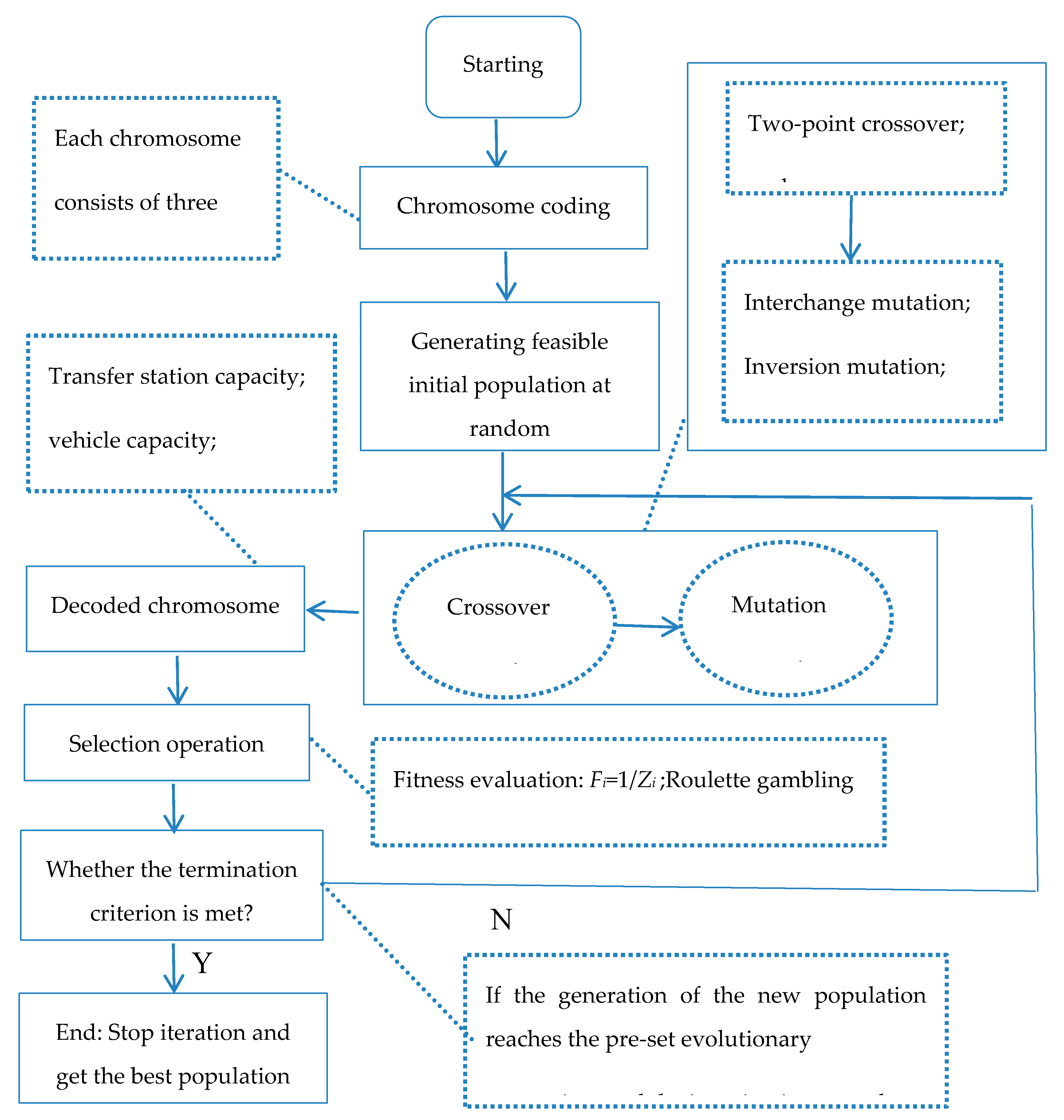
Based on the analysis of sub-cost in Section 3.4.1, a two-stage distribution location-routing model with the hard time window constrains for city cold-chain logistics is established as follows:

$${Minz}_1=C_1+C_1^{\prime }+C_2^{\prime }+C_3+C_3^{\prime }+C_4+C_5$$

(7)

Subject to:

$${\displaystyle \sum _{i\in M_1}{X}_i^k{q}_i\le }{Q}_1\hspace{1em}\hspace{1em}k\in K$$

(8)

$${\displaystyle \sum _{i\in N_g}{q}_i^{\prime }{y}_{ig}^l\le Q_2}\hspace{1em}g\in M_1,l\in L_g$$

(9)

$${\displaystyle \sum _{j\in M}{X}_{ij}^k=}{X}_i^k\hspace{1em}i\in M;k\in K$$

(10)

$${\displaystyle \sum _{i\in M}{X}_{ij}^k=X_j^k,}\hspace{1em}j\in M;k\in K$$

(11)

$${\displaystyle \sum _{i\in N_g}{\displaystyle \sum _{g\in M_1}{x}_{ijg}^l=y_{jg}^l}}\hspace{1em}j\in N_g,l\in L_g$$

(12)

$${\displaystyle \sum _{j\in N_g}{\displaystyle \sum _{g\in M_1}{x}_{ijg}^l=y_{ig}^l}}\hspace{1em}i\in N_g,l\in L_g$$

(13)

$${\displaystyle \sum _{g\in M_1}{\displaystyle \sum _{l\in L_g}{y}_{jg}^l}}=1\hspace{1em}j\in N_g$$

(14)

$${\displaystyle \sum _{j\in N_g}{x}_{ijg}^l={\displaystyle \sum _{j\in N_g}{x}_{jig}^l\le 1\hspace{1em}i=g\in M_1;l\in L_g}}$$

(15)

$${\displaystyle \sum _{j\in M_1}{X}_{ij}^k={\displaystyle \sum _{j\in M_1}{x}_{ji}^k\le 1\hspace{1em}i=0;k\in K}}$$

(16)

$${\displaystyle \sum _{i\in N_g}{q}_i^{\prime }{y}_{ig}\le Z_g{q}_g}\hspace{1em}g\in M_1$$

(17)

$$E{T}_i\le t_i^l\le L{T}_i$$

(18)

The objective function of the model is shown in (7). Constraint (8) shows that a vehicle cannot exceed its maximum load in the first level distribution. Constraint (9) shows that vehicle can not exceed its maximum load in the second-level distribution. The first stage of distribution flow balance is shown in (10) and (11). The second-stage of distribution flow balance is shown in (12) and (13). Constraint (14) shows that there is only one refrigerated vehicle providing a delivery service for one customer. As per constraints (15) and (16), the refrigerated vehicles starting from a transfer station must return to the same after serving the customer, and the refrigerated vehicles starting from the distribution center must return to the distribution center after serving transfer stations. The total customer requirements assigned to a transfer station must be lower than or equal to the storage capacity of the transfer station, which is imposed by (17). Constraint (18) represents the time window for customer i.

4. Algorithm Design

Two-stage distribution location-routing belong to the NP-Hard problem, so we use heuristic algorithms to solve this problem. A hybrid genetic algorithm is proposed in the paper combining heuristic rules and distance clustering. The flow chart of the algorithm is shown in Figure 2.

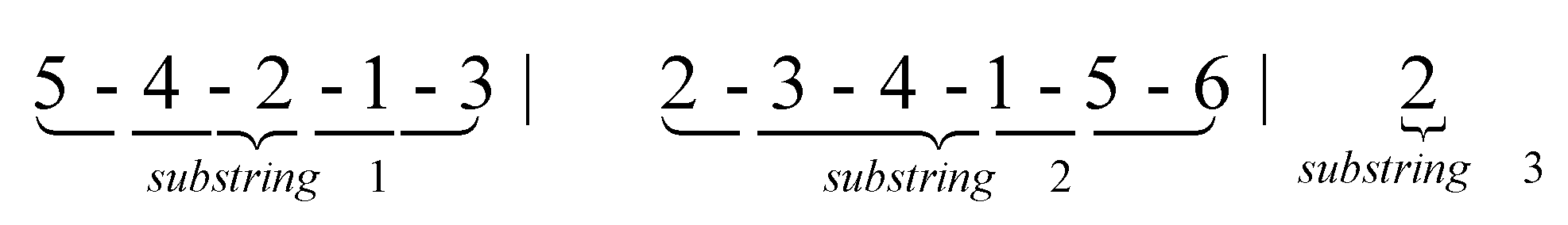
4.1. Chromosome Coding

Each chromosome consists of three sub-strings: Sub-string 1 involves encoding length J. The integer of gene 1 − J is a non-repetitive sequence, representing the priority selection order and delivery order of the transfer station. Sub-string 2 is encoded as an integer with length N and gene 1 − N, representing the distribution order of the demand points. Sub-string 3 is encoded as an integer code of length 1, indicating the number of transfer station selected. For example, when J = 5 and N = 6, namely, there are 5 transfer station and 6 customer point, for the chromosome shown in Figure 3, the priority of the transition to be selected is 5, 4, 2, 1, 3. The distribution path of the demand points is 2-3-4-1-5-6; 2 indicates that the first two bits of the first layer of coding are selected to set up a transfer station. Moreover, 5, 4 coded in the first layer is the order of distribution of the transfer station.

4.2. Generate the Initial Population at Random

Genetic algorithm starts from the population of the problem solutions, so it is necessary to generate an initial population as the starting point of evolution. According to the encoding method, N chromosomes are randomly generated.

4.3. Crossover Operation

To maintain the diversity of the population, we conducted crossover operations for each sub-string in the chromosome. Two-point crossover operation is carried out in sub-string 1. Cycle crossover operation is chosen to perform on sub-string 2. Two-point crossover operation is used in sub-string 3. The detailed description of crossover operation is as follows:

(1)

Crossover operation of sub-string 1

Two-point crossover: firstly, two chromosomes are randomly selected as the parent, and generating two random natural numbers r1 and r2. Secondly, the gene fragments between r1 and r2 of two parent chromosomes are exchanged, two offspring chromosomes are obtained. Finally, the chromosomes of the two offspring are modified so that no conflict occurs. For example, parent chromosome 1: 1 3 2 5 4, parent chromosome 2: 1 2 4 5 3, random numbers r1 = 2, r2 = 4. The offspring chromosomes after crossing are offspring chromosome 1: 1 2 4 5 4 and offspring chromosome 2: 1 3 2 5 3. Finally, two new offspring chromosome are obtained by repairing, new offspring chromosome 1: 1 2 4 5 3, new offspring chromosome 2: 1 3 2 5 4.

(2)

Crossover operation of sub-string 2

Cycle crossover: firstly, a cycle will be found according to the corresponding gene position of the parent chromosome. Secondly, the circulating gene is replicated to the offspring. Thirdly, the remaining genes are identified for the offspring, and the remaining genes outsides the parent chromosome cycle are used to fill with the original offspring. Finally, forming new descendants. For example: Firstly, parent chromosome 1: 2 7 5 6 4 8 9 1 3, parent chromosome 2: 4 3 6 8 9 7 1 2 5, find cycle 1: 2 4 9 1 2, cycle 2: 4 2 1 9 4. Secondly, offspring chromosome 1: 2 * * * 4 * 9 1 *, offspring chromosome 2: 4 * * * 9 * 1 2 *. Thirdly, parent 1 remaining chromosome: * 3 6 8 * 7 * * 5, parent 2 remaining chromosome: * 7 5 6 * 8 * * 3. Finally, new offspring chromosome 1: 2 3 6 8 4 7 9 1 5; new offspring chromosome 2: 4 7 5 6 9 8 1 2 3.

(3)

Crossover operation of sub-string 3

Two-point crossover: random selection of two chromosomes as parents and two offspring chromosomes are obtained by direct exchange of two parent chromosomes. For example, select two parent chromosomes 1 and 2, the chromosomes of the crossed offspring are 2 and 1.

4.4. Mutation Operation

To maintain the diversity of the population, we conducted mutation operation for each sub-string in the chromosome. Interchange mutation operation is carried out in sub-string 1. Inversion mutation operation is chosen to perform on sub-string 2. Single-point mutation operation is used in sub-string 3. The detailed description of mutation operation is as follows:

(1)

Mutation operation of sub-string 1

Interchange mutation: Two random points are selected in the encoding string, and their positions are swapped. For example, select exchange points 3 and 7 from chromosomes 1 4 3| 9 2 6 7| 5 8, the chromosome obtained after exchange mutation is 1 4 7| 9 2 6 3| 5 8.

(2)

Mutation operation of sub-string 2

Insertion mutation: randomly select two position points and insert the number of the first position point of the code string into the front of the second position in the code string. For example, we randomly select gene 4 from parent chromosome 1 4 |3 5 7 6| 2 9 8, and randomly select an insertion point 6, then the chromosome obtained after inserting the mutation is 1 3 5 7 4 6 2 9 8.

(3)

Mutation operation of sub-string 3

Single point mutation: the gene is mutated by random variation. For example, the parent chromosome is 3, the chromosome of offspring is 2 after single point mutation.

4.5. Decoding Chromosome

The chromosomes are decoded to determine the priority selection order and distribution order of the transit point, distribution order of each demand point, and number of transit points. According to the principle of distance clustering and capacity of the transit points, each demand point is allocated to the selected transition point successively. Moreover, the route is divided according to the limit of the vehicle capacity, and vehicles are assigned to each transit point to cover all the demand points allocated to the transit point.

4.6. Calculating Individual Fitness Value

The calculation formula for the individual fitness value is $F_i=1/Z_i$, where $F_i$ represents the fitness value of the i-th individual, and $Z_i$ represents the target function value of the i-th individual.

4.7. Selection Strategy Operation

Selection is the process of selecting the best individuals from the current population to produce a new population. We use the roulette selection strategy to select in this paper. The roulette selection is also known as proportional selection operator, and is to calculate the probability of each individual based on the fitness value of the individual. According to this probability, individuals are randomly selected to form the offspring population. This operation is repeated until the size of new population is identical to the original population size.

4.8. Algorithm Termination Condition

If gen > maxgen, output the best solution; this marks the end of the algorithm. Otherwise, let gen = gen + 1 and proceed to Step 4.

5. Description of Experiment and Analysis of Experimental Result

In the section, we use a randomly generated example to verify the validity of the model and the algorithm. Section 5.1 describes the experimental data generation and the parameters selection of the model. The experimental results are analyzed in Section 5.2. Comparative analysis of the results using different objective function of two-stage location-routing is shown in Section 5.3. In Section 5.4, we analyze the difference of distribution cost between two-stage vehicle routing and single-stage vehicle routing. The proposed algorithm and computations are carried out using MATLABR2017a package; all numerical experiments referenced in this paper are evaluated by a computer with windows7-x32 operating system, intel core i7 CPU @ 3.4 GHZ and 4 GB memory.

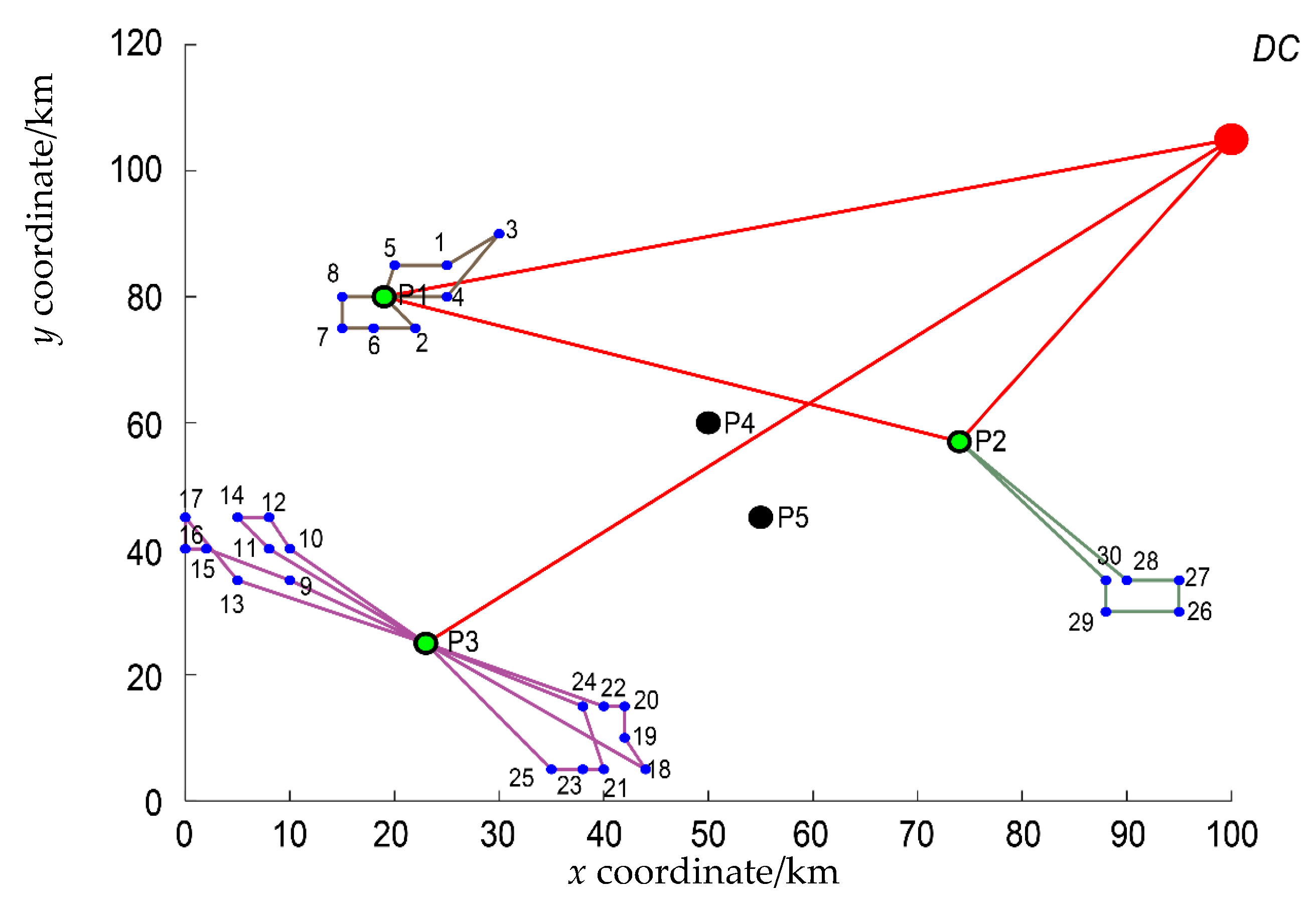
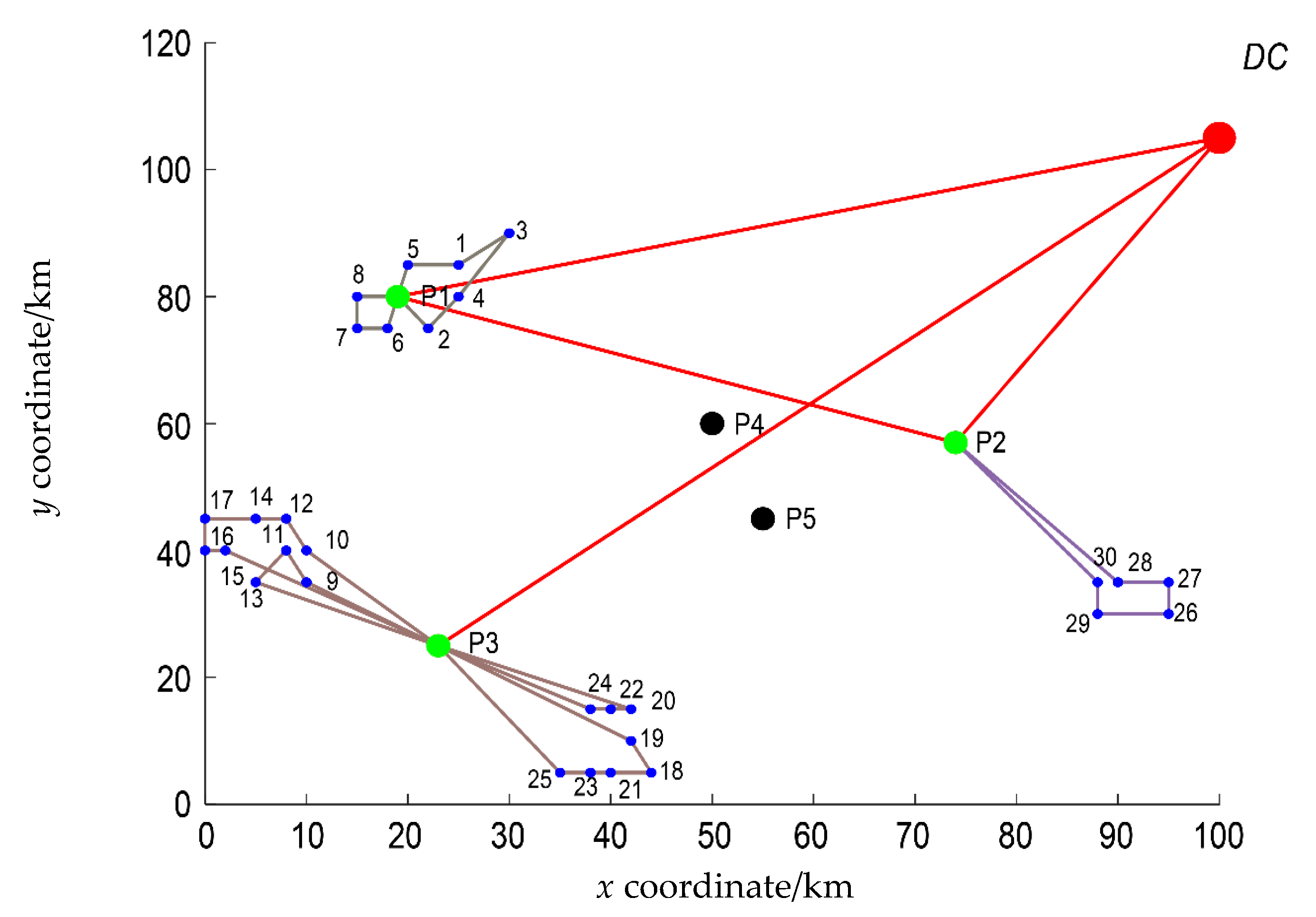
5.1. Experimental Data and Parameter Values

The test data for the calculation example are obtained using random generation. The customer demand is generated randomly within the interval [0, 3], and the x and y coordinates of the customer’s position are generated randomly in [0, 100]. The service time is set to 10 min. The data pertaining to the distribution center and transit point are set according to practical significance.

Table 1. Distribution center and transfer stations data.

	x Coordinate/km	y Coordinate/km	Capacity/t		x Coordinate/km	y Coordinate/km	Capacity/t
DC	100	105	100	P1	19	80	15
P2	74	57	20	P3	23	25	25
P4	50	60	15	P5	55	45	20

and

Table 2. Demand information of customers.

Demand Point	x Coordinate	y Coordinate	Quantity Demand	Time Window	Demand Point	x Coordinate	y Coordinate	Quantity Demand	Time Window
1	25	85	1.75	5:30–11:00	2	22	75	1.75	7:00–10:30
3	30	90	2.25	5:30–8:30	4	25	80	0.5	6:00–9:00
5	20	85	0.75	6:10–10:00	6	18	75	2	6:30–10:20
7	15	75	1.75	7:00–11:30	8	15	80	2.25	7:00–10:00
9	10	35	1.25	6:40–9:30	10	10	40	1	6:30–11:40
11	8	40	2	7:00–12:30	12	8	45	0.75	7:00–12:00
13	5	35	0.75	7:00–10:30	14	5	45	1.25	7:00–11:00
15	2	40	1.25	7:00–12:00	16	0	40	2.25	6:20–11:30
17	0	45	1	6:40–11:30	18	44	5	1	7:00–12:00
19	42	10	0.25	6:00–11:00	20	42	15	2.25	7:00–11:00
21	40	5	1.5	5:30–11:00	22	40	15	2.25	7:00–10:30
23	38	5	0.5	5:30–8:30	24	38	15	2.25	6:00–9:00
25	35	5	2	6:10–10:00	26	95	30	2.25	6:30–10:20
27	95	35	1.5	7:00–11:30	28	90	35	2	6:40–9:30
29	88	30	1	6:30–11:40	30	88	35	1	7:00–12:30

list the detailed data. The distribution center is represented by DC, the transit point by Pi (i = 1,2,3,4), and the customer point by natural numbers 1, 2, 3, …, 30. The values of the parameters in the model are: $Q_1=25$ t; $Q_2=8$ t; $c_1=2$ yuan/km; $c_2=1.5$ yuan/km; $c_1^{\prime }=100$ Yuan/h; $c_2^{\prime }=60$ yuan/h; when $Q_1=25$ t, $W_1=1.2$ kg/h, $W_2=2.2$ kg/h, $v_1=60 km/h$; when $Q_2=8$ t, $W_1=0.8$ kg/h, $W_2=1.8$ kg/h; $v_2=40 km/h$; $P_1=4000$ yuan/t; ${\theta }_1=0.003$; ${\theta }_2=0.002$; ${\theta }_3=9.3$ yuan/kg; ${\lambda }_1=50$ yuan; and $v_3=40$ t/h. The values of the parameters in the algorithm are: the initial population size N = 100, gen = 1, max iteration number maxgen = 500, crossover probability $p_c=0.8$, and mutation probability $p_m=0.1$.

5.2. Analysis of Experimental Result

MATLAB programming was used to implement the above algorithm, and the test example was solved for 30 iterations. The calculation time was within 30 s, and the calculation efficiency was high. The calculation results were relatively stable: in the solution of the 30 times, all choose transit point 1, 2, and 3 for transit, the total number of paths is 9, the average value of the objective function is 8045.5, and the values of the objective function of the worst solution and the optimal solution are 8193 and 7969, respectively (the deviations from the mean are only 1.8% and 0.9%). The optimal solutions correspond to the primary path 2: namely DC-P1-P2-DC, DC-P3-DC. There are seven secondary paths, namely P1-8-7-6-2-P1, P1-5-1-3-4-P1, P2-28-27-26-29-30-P2, P3-24-21-23-25 -P3, P3-22-20-19-18-P3, P3-11-14-12-10-P3, and P3-9-15-16-17-13-P3. The optimal solutions meet the requirements of the hard time window. Figure 4 and Figure 5 show the convergence of the optimal solution and the optimal results of the example.

5.3. Comparative Analysis of the Results under Different Objective Function of Two-Stage Location Routing

The proposed algorithm is employed to optimise the objective functions of the minimum total cost and minimum travel distance. MATLAB software was run 30 times to obtain the optimal distribution path number and cost of all levels, as listed in

Table 3. Two-stage location-routing under different optimisation targets.

Optimisation Target	Distribution Layer	Number of Paths	Travel Distance/km	Travel Time/min	Transportation Cost/yuan	Refrigeration Cost/yuan	Damage Cost/yuan	Total Cost/yuan
Minimum travel Distance	First Stage	2	421.05	487.42	1654.46	1428.82	-	3083.28
	Second Stage	7	351.05	826.58	1357.17	687.48	760.67	2805.32
	Total	9	772.1	1314	3011.63	2116.3	760.67	5888.6
Minimum Total Cost	First Stage	2	421.05	487.42	1654.46	1428.82	-	3083.28
	Second Stage	7	369	853.5	1407.01	633.81	633.25	2674.07
	Total	9	790.05	1340.92	3061.47	2062.63	633.25	5757.35

, and, Figure 5 and Figure 6. When taking minimum travel distance as the objective function (Figure 6), the optimal solution is the primary path 2: namely DC-P3-DC, DC-P1-P2-DC, there are seven secondary paths, namely P1-8-7-6-P1, P1-5-1-3-4-2-P1, P2-28-27-26-29-30-P2, P3-24-22-20-P3, P3-25-23-21-18-19-P3, P3-9-11- 13-P3, and P3-10-14-12-17-16-15-P3.

Different objective functions have no impact on the transfer cost, total number of paths, and cost of the first-level paths. The transit cost is 2212.5 yuan, the total number of routes is 9, and the cost value, delivery distance, and travel time in the first-stage routes the same. The second-stage cost and routes are different for different objective functions. The objective function with the shortest distance saves 17.95 km in distance and 26.92 min in time compared to that with the minimum total cost, incurring 131.25 yuan more in total cost. Therefore, cold-chain participants can choose different route schemes to maximise their interests. If the carrier is the main participant, the route scheme with the lowest total cost may be the best choice. If logistics outsourcing is involved, the shortest travel distance may be the best choice for logistics providers.

5.4. Comparisons of Two-Stage Distribution Location Routing and Single-Stage Vehicle Routing

A comparison between Table 3 and

Table 4. The single-stage vehicle routing cost details.

Vehicle Capacity/t	Transportation Cost/yuan	Refrigeration Cost/yuan	Damage Cost/yuan	Total Cost/yuan
25 t	4035.03	2871.21	1094.74	8001.18
8 t	6051.54	1666.79	967.35	8685.68

shows that, for single-stage vehicle paths, when the distribution vehicle capacity is 25 t, the vehicle path cost is 8001.18, when the distribution vehicle capacity is 8 t, the vehicle path cost is 8685.68, and for two-stage distribution location-routing, vehicle routing cost is 5757.35, transfer cost is 2212.5, total cost is 7969.85. Thus, the single-stage vehicle path increases the vehicle path cost. Despite the cost savings representing a small percentage of the total cost, the large activity of two-stage distribution in a big city may represent a substantial benefit per year. Beside the significant economic advantages yielded by this kind of distribution approach, two-stage distribution systems may result in being more efficient with respect to standard approaches and also from an environmental point of view. In addition, with the gradual implementation of vehicle restriction policy in China, the two-stage distribution scheme established can avoid large vehicles in the city center in this paper, thus saving distribution cost and improving operating profits.

6. Conclusions

Based on the characteristics of city logistics distribution, we have established two-stage distribution location-routing model with the hard time window for city cold-chain logistics. Different vehicle types were considered for the different distribution tasks. In order to solve the model, we designed a hybrid genetic algorithm, and the model and algorithm were verified through a random generated example. The effects of different objective functions on the location routing and total distribution cost were analysed, and the objective functions had no effect on the transfer location selection, but did have on the total cost. Therefore, different distribution optimisation schemes were proposed for different distribution subjects. A two-stage distribution location-routing problem and a single-stage vehicle-routing problem were compared and analysed. The results showed two-stage distribution scheme can help reduce overall distribution cost, indicating that the two-stage location-routing system is more feasible and effective. In conclusion, the two-stage location-routing model can provide a theoretical reference for the planning of distribution networks in the field of cold-chain logistics.

The operating conditions of city logistics distribution networks are very complex. Therefore, in future research, real traffic conditions, including potential congestion, and feasible geographical locations for transfer stations should be considered in the distribution planning. For example, the introduction of a road congestion index into the model can help to better reflect the actual feasible solution. Also, additional problem formulations in two-stage distribution, such as bi-level optimization where lower and upper optimization tasks are considered, will be faced in the next steps of future works jointly with comparison exercises with exact solutions and solvers (e.g., CPLEX).

References

1. Taniguchi, E.; Thompson, R.G.; Yamada, T. New opportunities and challenges for city logistics. Transp. Res. Procedia 2016, 12, 5–13. [Google Scholar] [CrossRef] [Green Version]
2. Macharis, C.; Melo, S. City Distribution and Urban Freight Transport; Edward Elgar Publishing Limited: Cheltenham, UK, 2011. [Google Scholar]
3. Taniguchi, E.; Thompson, R.G.; Yamada, T. City Logistics Network Modeling and Intelligent Transport Systems; Elsevier: Oxford, UK, 2001. [Google Scholar]
4. Allen, J.; Anderson, S.; Browne, M.; Jones, P. A Framework for Considering Policies to Encourage Sustainable Urban Freight Traffic and Goods/Service Flows; Transport Studies Group, University of Westminster: London, UK, 2000. [Google Scholar]
5. Taniguchi, E.; Tamagawa, D. Evaluating city logistics measures considering the behavior of several stakeholders. J. East. Asia Soc. Transp. Stud. 2015, 6, 3062–3076. [Google Scholar]
6. Anand, N.; Quak, H.; Duin, R.V.; Tavasszy, L. City logistics modeling efforts: Trends and gaps – a review. Procedia Soc. Behav. Sci. 2012, 39, 101–115. [Google Scholar] [CrossRef] [Green Version]
7. Danielis, R.; Rotaris, L.; Marcucci, E. Urban freight policies and distribution channels: A discussion based on evidence from Italian cities. Eur. Transp. Transp. Eur. 2010, 46, 114–146. [Google Scholar]
8. Allen, J.; Browne, M.; Woodburn, A.; Leonardi, J. The role of urban consolidation centres in sustainable freight transport. Transp. Rev. 2012, 32, 473–490. [Google Scholar] [CrossRef]
9. Browne, M.; Sweet, M.; Woodburn, A.; Allen, J. Urban Freight Consolidation Centres Final Report. Transport Studies Group, University of Westminster, 2005; Volume 10. Available online: https://www.semanticscholar.org/paper/Urban-freight-consolidation-centres%3A-final-report-Browne-Sweet/4a1a5346e3a81d2f20102579a66fcb19f595cb65 (accessed on 13 December 2019).
10. Lagorio, A.; Pinto, R.; Golini, R. Research in urban logistics: A systematic literature review. Int. J. Phys. Distrib. Logist. Manag. 2016, 46, 908–931. [Google Scholar] [CrossRef]
11. Kijewska, K.; Iwa, S.; Kaczmarczyk, T. Technical and organizational assumptions of applying UCCs to optimize freight deliveries in the seaside tourist resorts of West Pomeranian region of Poland. Procedia Soc. Behav. Sci. 2012, 39, 592–606. [Google Scholar] [CrossRef] [Green Version]
12. Iwan, S.; Kijewska, K.; Johansen, B.G.; Eidhammer, O.; Małecki, K.; Konicki, W.; Thompson, R.G. Analysis of the environmental impacts of unloading bays based on cellular automata simulation. Transp. Res. Part D Transp. Environ. 2018, 61, 104–117. [Google Scholar] [CrossRef]
13. Simona, M. Multi-echelon distribution systems in city logistics. Eur. Transp. Transp. Eur. 2013, 1–13. [Google Scholar]
14. El-Ghazali, T. Metaheuristics: From Design to Implementation; John Wiley & Sons: Hoboken, NJ, USA, 2009; Volume 74. [Google Scholar]
15. Von Boventer, E. The relationship between transportation costs and location rent in transportation problems. J. Reg. Sci. 1961, 3, 27–40. [Google Scholar] [CrossRef]
16. Perl, J.; Daskin, M.S. A warehouse location-routing problem. Transp. Res. 1985, 19, 381–396. [Google Scholar] [CrossRef]
17. Li, J.; Chu, F.; Chen, H. A solution approach to the inventory routing problem in a three-level distribution system. Eur. J. Oper. Res. 2011, 210, 736–744. [Google Scholar] [CrossRef]
18. Prodhon, C. A hybrid evolutionary algorithm for the periodic location-routing problem. Eur. J. Oper. Res. 2011, 210, 204–212. [Google Scholar] [CrossRef]
19. Xu, J.H. Based on GA-PSO algorithm of fresh agricultural products location-routing problem optimization research. Logist. Eng. Manag. 2016, 38, 51–53+55. [Google Scholar]
20. Song, Q.; Liu, L.X. Research on multi-trip vehicle routing problem and distribution center location problem. Math. Pract. Theory 2016, 39, 103–113. [Google Scholar]
21. Zhao, Q.; Wang, W.; De, R.S. A heterogeneous fleet two-echelon capacitated location-routing model for joint delivery arising in city logistics. Int. J. Prod. Res. 2017, 56, 1–19. [Google Scholar] [CrossRef]
22. Wang, Y.; Assogba, K.; Liu, Y.; Ma, X.; Xu, M.; Wang, Y. Two-echelon location-routing optimization with time windows based on customer clustering. Expert Syst. Appl. 2018, 104, 244–260. [Google Scholar] [CrossRef]
23. Koç, Ç.; Bektaş, T.; Bektas, T.; Jabali, O.; Laporte, G. The fleet size and mix location-routing problem with time windows: Formulations and a heuristic algorithm. Eur. J. Oper. Res. 2016, 248, 33–51. [Google Scholar] [CrossRef] [Green Version]
24. Leng, L.; Zhao, Y.; Wang, Z.; Zhang, J.; Wang, W.; Zhang, C. A novel hyper-heuristic for the biobjective regional low-carbon location-routing problem with multiple constraints. Sustainability 2019, 11, 1596. [Google Scholar] [CrossRef] [Green Version]
25. Yu, V.F.; Lin, S.Y. Solving the location-routing problem with simultaneous pickup and delivery by simulated annealing. Int. J. Prod. Res. 2016, 54, 526–549. [Google Scholar] [CrossRef]
26. Zhao, Y.; Leng, L.; Zhang, C. A novel framework of hyper-heuristic approach and its application in location-routing problem with simultaneous pickup and delivery. Oper. Res. 2019, 1–34. [Google Scholar] [CrossRef]
27. Yang, H.X.; Li, H.D.; Du, W.; Zhang, H. Research on location selection of perishable dairy products distribution center based on two-stage distribution. Comput. Eng. Appl. 2015, 51, 239–245. [Google Scholar]
28. Zhao, S.; Zhuo, F.U. Distribution location routing optimization problem of food cold chain with time window in time varying network. Appl. Res. Comput. 2013, 30, 183–188. [Google Scholar]
29. Zheng, J.; Li, K.; Wu, D. Models for location inventory routing problem of cold chain logistics with NSGA-ⅡAlgorithm. J. Donghua Univ. Engl. Ed. 2017, 4, 50–56. [Google Scholar]
30. Wang, S.; Tao, F.; Shi, Y. Optimization of location–routing problem for cold chain logistics considering carbon footprint. Int. J. Environ. Res. Public Health 2018, 15, 86. [Google Scholar] [CrossRef] [Green Version]
31. Liu, G.H.; Xie, R.H.; Zou, Y.F.; Huang, X. Study on evaluation system of energy consumption of food refrigerated transport equipment. Guangdong Agric. Sci. 2013, 40, 176–189. [Google Scholar]
32. Wang, G. Optimization Research of Common Distribution Routing Problem of Cold Chain Logistics Based on Joint Distribution Mode. Master’s Thesis, Beijing Jiaotong University, Beijing, China, 2018. [Google Scholar]
33. Shi, C.C.; Wang, X.; Ge, X.L. Research on vehicle scheduling problem of multi-distribution centers with time window. Comput. Eng. Appl. 2009, 45, 21–24. [Google Scholar]
Figure 1. Schematic map of location-routing in two-stage distribution.
Applsci 10 02564 g001
Figure 2. Flow chart of hybrid genetic algorithm.
Applsci 10 02564 g002
Figure 3. Chromosome coding example.
Applsci 10 02564 g003
Figure 4. Algorithm convergence curve.
Applsci 10 02564 g004
Figure 5. Minimum total cost two-stage location-routing diagram.
Applsci 10 02564 g005
Figure 6. Shortest distance two-stage location-routing diagram.
Applsci 10 02564 g006