Adaptive Visual Servoing Control for Hoisting Positioning Under Disturbance Condition

Abstract

This paper proposes a visual servo scheme for hoisting positioning under disturbance conditions. In actual hoisting work, disturbances such as equipment and load vibration are inevitable, which brings challenges to the development of a visual servo for hoisting positioning. The main problems are as follows: (1) the correlation between visual error and disturbance is not considered or well resolved; (2) the disturbance has a great influence on the control stability, but it is difficult to model. At present, there is no detailed research on the above problems. In this paper, the visual error is defined by the image error of the feedback signal based on dynamic equations containing disturbances. An adaptive sliding mode control algorithm is employed to decrease the influence of external disturbance, and the coefficient of the slide surface is established based on the adaptive gain. In view of the belief that it is difficult to model disturbance terms, a nonlinear disturbance observer is introduced to obtain equivalent disturbance. On this basis, an adaptive control algorithm with disturbance compensation is proposed to improve the robustness of the visual servo system. We use Lyapunov’s method to analyze the stability conditions of the system. Compared with the other state-of-the-art methods, the simulation results show that our method has superior performance in convergence, accuracy, and restraining disturbance. Finally, the proposed algorithm is applied to the hoisting platform for experimental research, which proves the effectiveness of the controller.

1. Introduction

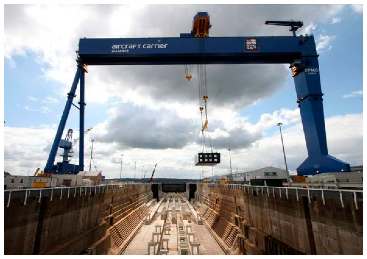
Automatic hoisting positioning technology is the main component of unmanned crane technology. The research into automatic hoisting positioning technology is conducive to the development of intelligent cranes and technology upgrading, which are key in the technology of cranes in the future. The key to improving the automation level of the hoisting operation is to realize accurate hoisting positioning (Figure 1). Port hoisting, prefabricated building construction and the installation of large energy and power equipment all need accurate hoisting positioning. The traditional positioning method is to install an absolute value encoder [1] on the driving shaft of the crane. The absolute value encoder converts the rotation of the shaft into the moving distance and transmits it to the control system, which judges whether the equipment arrives at a designated position. For conventional cranes, this design is feasible and widely used. However, when it is used in high-precision cranes, deviations occur. The reason is that the driving wheel slips, and the wheel shaft rotates but the crane does not move, resulting in the instability of the positioning system. In order to solve the problem of low positioning accuracy, the rack and pinion positioning system is introduced into the hoisting positioning technology. 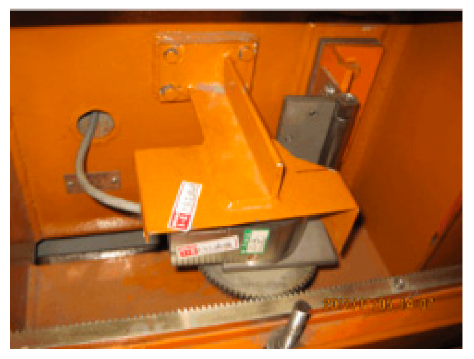The rack and pinion positioning system [2] improves the positioning accuracy, and is widely used in subsequent nuclear power projects. However, the rack and pinion positioning system (Figure 2) still faces many challenges: the rack needs to be laid out to its full length, and the machining accuracy of the rack itself is too high, which brings great trouble to the engineers. For a crane with long travel distances and precise positioning, researchers tried to use a cable encoder, which consists of a cable box and an absolute value encoder. As the cable is pulled out and retracted, the encoder measures the number of turns of the drum in the cable box and converts it into a measurement signal to output to the system. In the actual project, it is found that the cable is easily damaged in the installation and commissioning processes. Moreover, the magnetic ruler system [3] has been developed and applied to hoisting positioning, but it has not been popularized because of the limitations of the working environment. Radiofrequency technology [4] has also been used in this field, but its performance was greatly discounted due to signal shielding and interference.

As a non-contact sensor, the camera can be used as the eye of the hoisting equipment to increase the ability of environmental perception. With this method, we can control the crane in a closed loop. In recent years, visual servoing has ben widely used in trajectory tracking and positioning technology [5,6]. However, in the hoisting and positioning operation, the external environment is unstable, and is easily affected by wind load, equipment vibration and other factors, which bring disturbances to the visual servo system, resulting in low accuracy of positioning, slow response speed and other problems. Therefore, in this paper, research into visual servo control under disturbance conditions is carried out.

2. Literature Review

As in [5], the visual servo control uses data from a vision system to control the movement of robot or mobile devices. In general, there are two kinds of visual servo control modes, according to the installation position of the camera. According to the fixation of the camera, visual servo can be divided into two categories, one is where the camera is placed directly onto a robot or robotic arm, called “eye-in-hand”, the other is where the camera is fixed at the workspace, called “eye-to-hand”.

Kinematic and dynamic modeling under the disturbance condition is key to completing the relationship between visual error and disturbance. For a visual servo system, a variety of modeling methods are constantly applied and proposed, and the interaction with the external environment is considered. Dong [7] used vision measurement technology and the Extended Kalman Filter (EKF) algorithm to estimate the pose and motion parameters of the target. Based on the target pose and motion parameters, the incremental inverse kinematics model was established to obtain the desired position of the end effector. Different from the above control method, which only considers the system kinematics, Krupínski [8] studied the kinematics and dynamics of the whole system, including nonlinear, coupling effect, interaction with the external environment and other factors, and applied the scene feedback information of the homography matrix between different images to the system dynamics to improve the control stability of the system. Dynamic modeling under different conditions is the key to solving the stability problem, and the state feedback controller is widely used for stability control [9]. Hu [10] proposed a fault-tolerant control scheme based on a disturbance observer, which can effectively suppress the external disturbance and reduce the impact of actuator failure on the control system. Based on the disturbance observer, the uncertainty caused by external disturbance or actuator failure is established and compensated. Aiming to solve the the problem of control error convergence in a closed-loop control system, an attitude stabilization control system based on integral sliding film was proposed. Fan [11] proposed an Model Predictive Control (MPC) control strategy, including an auxiliary state feedback controller and robot system. The kinematic state error of the nominal system was transformed into a chain system to solve the MPC optimization problem of the nominal system and generate the optimal state trajectory of the robot system. Ke [12] used MPC to stabilize the physical constraints of the robot system; the kinematic equation of the nonholonomic chain system was transformed into the form of skew symmetry, and the exponential decay phase was introduced to solve the uncontrollable problem of the system. Obviously, this can be used as a reference to prove that it is possible to transform the kinematic state error into the chain optimization problem.

It is necessary to improve the robustness of the visual servo system in the presence of uncertainty [13,14,15,16]. Under the uncertainty of system dynamics and vision framework, Zergeroglu [17] studied the control of planar mobile devices, in order to compensate the uncertainty of the system; a robust controller was designed to ensure the final uniform boundedness of the position tracking. Ma [18] studied the singularity and local extremum in visual servo control, and proposed a robust design strategy to suppress image noise and external disturbance, so as to ensure the internal stability of the closed-loop system. However, when the external interference changes, the effect of this robust design strategy is not ideal. In the research, the constraint optimization problem is transformed into a H∞ control framework, which improves the anti-interference of the system. It means that the research system not only contains uncertainty, but also requires to a strongly conservative performance index to be achieved.

In order to obtain better dynamic stability performance in a camera robot system, Li [19] proposed a new Lyapunov-positive definite function based on the asymptotic stability of the visual servo system. Considering the more complex situation of visual systems, including the uncertainty of system dynamics and camera parameters, the asymptotic convergence of image tracking errors was proved. Liu [20] focused on the research of ship motion control, and put forward a scheme based on the sliding mode control. With the aim of studying wave disturbance, he introduced the nonlinear disturbance observer, and studied its suppression characteristics. The stability of the above studies are, respectively, observed from two different perspectives—aspects of visual function and disturbance suppression—but the environmental limitations are more prominent. Obviously, the nonlinear problem of the visual servoing system is inevitable [21,22,23]. Elastic objects will deform under the condition of complete constraint, which will bring more nonlinear problems to visual servo control. David [21] proposed an uncalibrated algorithm based on Lyapunov to estimate the visual Jacobian matrix in the deformed state; he applied this method to a clamping operation based on visual servo control, and combined the pose information of the gripper with the visual information to realize the recognition and control of its pose. Xu [22] extracted sensitive features from image information to meet the requirements of position and direction control. The direction and position of the target were controlled by the idea that the target size is sensitive to the depth of the image. The feature translation caused by the rotation process was used as compensation, and the image depth was estimated by the interaction matrix and the change in the image features. Too much dependence on camera-sensitive features, when the delay is too large, it is likely to cause data distortion. Aiming at solving the control problem of multi-camera visual servo control systems, Kornuta [23] proposed a design method based on the embedded concept, and defined each subsystem in the multi-level system structure according to the conversion function. The accuracy of the multi camera system was limited, and the processing load of the system was increased. In recent years, machine learning methods such as neural networks have been used to solve various nonlinear problems [24,25]. Gao [26] proposed a vision servo (IBVS) dynamic positioning strategy. In the speed-tracking loop of the control system, an adaptive controller based on a neural network was designed. With the premise of ensuring the convergence of speed tracking error, the influence of cost function, the dynamic model and the speed reference model on system performance was studied compared to other schemes. Considering the dynamic and nonlinear problems of the system, Wang [27] proposed a vision servo scheme based on a neural network. An adaptive neural network was used to fit the unknown dynamic model. The advantage of this scheme is that it solves the problem of nonlinear effect of output. The controller based on neural network improves the control stability, but puts forward higher requirements for neural network construction. In the application of photometry in visual servo systems, the image changes because of the appearance and disappearance of some scenes [28]. Omar [29] focused on the research of visual servo technology based on photometric moment, and proposed a relatively direct and simple method that does not need feature extraction, visual tracking and image matching in traditional visual servo technology. The challenge of this method is that when the appearance of the image changes or partially disappears, its stability is difficult to guarantee. In the process of visual servo control using the whole photometric image information as a dense feature, the redundancy of visual information makes the convergence domain very small. Nathan [30] proposes an analytic visual servo based on Gaussian mixture to expand its convergence region. When the initial position is far away, it can still achieve stable speed control and converge to the desired position. In the motion control of a wheel robot based on a visual servo, the center position of the visual system is mostly the same as the center position of the robot body, but some settings that deviate from the center position of the robot are conducive to its motion, which will bring deviation to the visual system, resulting in the convergence failure of the visual error. In order to solve this problem, Qiu [31] designed a motion tracking method based on visual servo, which deviated from the center of the robot body, to solve the influence of the translation of the uncalibrated camera on the parameters of the visual system. In the visual servo control of most mobile robots, the trajectory and the desired position image must be given. Li [32] designed a positioning control scheme based on monocular vision, defined the image reference frame by using the visual target and plane motion constraints, proposed the attitude estimation algorithm of the robot relative to the image of desired pose, and constructed the updated rate of unknown feature parameters. However, when the visual target and motion constraint parameters change, the reference frame will change and the control precision will be affected.

This paper researches the hoisting positioning technology based on visual servo control under the disturbance condition and focuses on solving the following two puzzles: (1) the correlation between visual error and disturbance is not considered or well resolved; (2) the disturbance has a great influence on the control stability, but it is difficult to model. In this paper, the visual error model is defined by the image error of a feedback signal based on dynamic equations containing disturbance. To solve the problem of the disturbance term being difficult to model, the nonlinear disturbance observer is employed to obtain equivalent disturbance and an adaptive control algorithm, while disturbance compensation is proposed.

The organization of this paper is as follows. Section 3 depicts the problem description, including dynamics modeling, and IBVS modeling. In Section 4, we describe the visual servo control based on adaptive sliding mode control (SMC), then propose the control law with disturbance compensation, and give the stability analysis based on Lyapunov’s theory. Simulations are conducted in Section 5, which depicts the superiority of the proposed method against the other methods. Section 6 represents the experimental results of two projects with different initial positions. Finally, Section 7 contains a summary and outlook.

3. Materials and Methods

3.1. Dynamics Modeling

The schematic model is shown in Figure 3. The hoisting platform has four degrees of freedom, and the power device is composed of a Gantry driver and a Trolley driver. The driving force in each direction has no coupling effect. The state equation of hoisting equipment can be expressed as follows:

$$\dot{\eta }=\mathrm{T}({\eta }_b)\mathrm{v}$$

(1)

where $\eta ={\left[x,y,z,\phi ,0,0\right]}^{\mathrm{T}}\in {ℝ}^6$ represents the state vector of the end-effector, which contains the displacement vector ${\eta }_a={\left[x,y,z\right]}^{\mathrm{T}}$ and the angle vector ${\eta }_b=[\phi ,0,0]$. $\mathrm{v}=[v_x,v_y,v_z,{\omega }_{\phi }{,0,0]}^{\mathrm{T}}\in {ℝ}^6$ represents the velocity vector. $\mathrm{T}(\cdot )$ is the transformation matrix related to the body-fixed velocities and the global pose rates [25].

In an ideal state, the dynamic equation of the hoisting mechanism is expressed as follows:

$$M(\eta )\dot{\mathrm{v}}+C(\eta ,\mathrm{v})\mathrm{v}+G(\eta )=Q$$

(2)

$M(\cdot )>0$ is the positive definite inertial matrix of the system. $C(\cdot )$ is the corresponding Coriolis and centripetal matrices. $G(\cdot )$ represents the gravitational vector and Q represents the control vector, respectively.

However, in the actual hoisting positioning project, considering the nonlinear, uncertain and external interference factors in the model, the dynamic equation of hoisting equipment is described in the following form:

$$M(\eta )\dot{\mathrm{v}}+C(\eta ,\mathrm{v})\mathrm{v}+G(\eta )+\mathrm{D}(\mathrm{v})\mathrm{v}=Q+\tau$$

(3)

$D(\cdot )$ represents the damping matrix [21], and $\tau$ is the external disturbance.

3.2. IBVS Model

In this paper, the camera is fixed on the component in the form of “eye-in-hand”. C denotes the frame of the camera at its current pose, C* represents the frame of camera at the desired pose, G represents the world coordinate system. We set the camera coordinate frame to coincide with the hoisting component coordinate frame, where the hoisting component is considered to be consistent with the camera’s pose and speed (as Figure 4). Visual servo control uses a visual feedback signal as input, and calculates the end-effector velocity according to the Jacobian matrix. Therefore, it is necessary to associate the velocity of the end-effector in the camera coordinates with the robot reference system and establish the transformation relationship. A flow chart of the coordinate transformation is shown in Figure 5.

If $O_c$ and $O_c^{\ast }$ represent the feature points in the frame of C and C*, we define them as $O_c=(X_c,Y_c,Z_c{)}^{\mathrm{T}}\in {ℝ}^3$,$O_c^{\ast }=(X_c^{\ast },Y_c^{\ast },Z_c^{\ast }{)}^{\mathrm{T}}\in {ℝ}^3$. The derivative of $O_i$ can be denoted as follows.

$${\dot{O}}_c{=\mathrm{v}}_a+{\mathrm{v}}_b\times O_c$$

(4)

The camera coordinate system is transformed to the image physical coordinate system through the focal length diagonal matrix:

$$\{\begin{array}{l}{x}_c=\frac{f}{Z_c}{X}_c\\ y_c=\frac{f}{Z_c}{Y}_c\end{array}$$

(5)

In matrix form, it can be written as

$$Z_c\left[\begin{array}{l}x\\ y\\ 1\end{array}\right]=\left[\begin{array}{ccc}f& 0& 0\\ 0& f& 0\\ 0& 0& 1\end{array}\right]\left[\begin{array}{c}{X}_c\\ Y_c\\ Z_c\end{array}\right]$$

(6)

f > 0 is the camera focal length. ${\left[X_c,Y_c,Z_c\right]}^T$ represents the camera coordinates. ${\left[x,y,1\right]}^T$ represents the normalized physical coordinates of the image.

The image physical coordinate system is transformed to the pixel coordinate system through the pixel transformation matrix:

$$\{\begin{array}{l}u=\frac{x}{dx}+u_0={\alpha }_{1}x+u_0\\ v=\frac{y}{dy}+v_0={\alpha }_{2}y+v_0\end{array}$$

(7)

In matrix form, it can be written as

$$\left[\begin{array}{l}u\\ v\\ 1\end{array}\right]=\left[\begin{array}{ccc}\frac{1}{dx}& \gamma & u_0\\ 0& \frac{1}{dy}& v_0\\ 0& 0& 1\end{array}\right]\left[\begin{array}{c}x\\ y\\ 1\end{array}\right]$$

(8)

${\alpha }_1$,${\alpha }_2$ are the number of pixels per unit distance in two directions. $u_0$, $v_0$ are the pixel coordinates at the intersection of the camera optical axis and imaging plane.

According to the perspective projection principle, the feature points of the current and desired image coordinates can be expressed as follows:

$$s_i={[u_i,v_i]}^{\mathrm{T}}=\frac{F}{Z_i}{[x_i,y_i]}^{\mathrm{T}},s_i^{\ast }={[u_i^{\ast },v_i^{\ast }]}^{\mathrm{T}}=\frac{F}{Z_i}{[x_i^{\ast },y_i^{\ast }]}^{\mathrm{T}}$$

(9)

where, $u_i,v_i$ represent the coordinates of the feature points in the pixel coordinate system. $F=\left[\begin{array}{cc}{\alpha }_{1}f\hfill & 0\\ 0\hfill & {\alpha }_{2}f\end{array}\right]$.

According to (3), we can directly define the camera velocity as $\mathrm{v}=[v_x,v_y,v_z,{\omega }_{\phi }{]}^{\mathrm{T}}\in {ℝ}^4$, which consists of translational and rotational velocity under the disturbance condition.

In order to solve the problem of motion decoupling control, a vision servo decoupling control method [33] based on the line feature and inner region feature is adopted. The line direction feature is not affected by the camera’s translation movement, but only related to the camera’s rotation movement. The inner region feature is sensitive to the camera’s translation movement along the Z axis, but not affected by the rotation movement around the Z axis. Therefore, we use the inner region feature and the line feature as the visual features of the camera’s translation and rotation movement, respectively. The real-time target feature can be written as $s={[x_0,y_0,a,\theta ,0,0]}^{\mathrm{T}}$, where $x_0,y_0$ respectively correspond to the centroid coordinates of the circular feature, $a$ is the circular feature of the inner area, and $\theta$ corresponds to the direction angle value of any edge of the target area. The desired feature can be written as $s^{\ast }={[x_0{}^{\ast },y_0{}^{\ast },a^{\ast },{\theta }^{\ast },0,0]}^{\mathrm{T}}$.

Attitude control based on the line feature can be denoted as

$${\omega }_{\phi }=-{\lambda }_c{J}_c{}^{-}(\theta -{\theta }^{\ast })$$

(10)

$J_c{}^{-}$ is the Moore–Penrose pseudo-inverse of the Jacobian matrix $J_c$. ${\lambda }_c$ is the pose controller gain. The displacement velocity vector of the camera is defined as follows

$$v=v_{ca}+v_{\omega }$$

(11)

where $v_{ca}$ and $v_{\omega }$ are the camera translation velocities with the compensation of the inner region feature vector and the center of mass, as in [33].

Considering that the real-time target feature is $s$ and the desired target feature $s^{\ast }$, the feature error $e$ can be calculated as

$$e=s^{\ast }-s.$$

(12)

4. Controller Design

4.1. Adaptive Control Law

In this paper, the visual error model is defined by the image error of the feedback signal based on dynamic equations containing disturbance. Considering the local asymptotic stability of the visual servo system, the visual error signal is denoted as

$$\xi ={\widehat{J}}_c{}^{-}e$$

(13)

${\widehat{J}}_c{}^{-}$ is the Moore–Penrose pseudo inverse of the estimated Jacobian matrix ${\widehat{J}}_c$.

Here, we use an estimation method [34] to obtain the interaction matrix ${\widehat{J}}_c^{}$. It is estimated to satisfy the following equation.

$$\dot{s}={\widehat{J}}_c^{}\mathrm{v}$$

(14)

Moreover, ${\widehat{J}}_c^{}\mathrm{v}$ can be written in the following linear form

$$\dot{s}={\widehat{J}}_c^{}\mathrm{v}=\Upsilon (\dot{\eta })\widehat{\vartheta }$$

(15)

where $\Upsilon (\dot{\eta })$ is a matrix without depending on the intrinsic and extrinsic parameters of the camera. $\widehat{\vartheta }$ is a vector where the components of ${\widehat{J}}_c^{}$ are listed [34].

In this paper, we adopt the method of image-based visual servoing (IBVS) [35]. In image-based visual servoing (IBVS), the control loop is directly closed in the image space of the vision sensor. Compared with position-based visual servoing and hybrid visual servoing, IBVS schemes get rid of 3-D reconstruction steps to compute the visual features.

The derivative of the visual error could be calculated by (13) as

$$\dot{\xi }=-{\widehat{J}}_c{}^{-}{J}_c\mathrm{v}+{\dot{\widehat{J}}}_c{}^{-}e$$

(16)

The estimation error of the Jacobian matrix is defined as

$${\tilde{J}}_c=J_c-{\widehat{J}}_c$$

(17)

If we substitute (17) into (16), we have

$$\dot{\xi }=-{\widehat{J}}_c{}^{-}{J}_c\mathrm{v}+{\dot{\widehat{J}}}_c{}^{-}e=-\mathrm{v}-o_{\xi }$$

(18)

where $o_{\xi }={\widehat{J}}_c^{-}{\tilde{J}}_c\mathrm{v}-{\dot{\widehat{J}}}_c^{-}e$.

The control purpose for the visual servo system is to use visual feedback $\xi$ to drive the target to the desired pose, like $\eta \to {\eta }^{\ast }$. At the same time, we should ensure the asymptotic stability of the system in the case of unknown and bounded uncertainties. Proportional control law is a widely used method and can be seen in most visual servo literature. However, it is difficult for a system using only proportional control law to obtain an ideal dynamic response. In this paper, sliding mode control (SMC) is used to compensate for the influence of external disturbance. The velocity control signal could be calculated from the visual system based on the inverse of the estimated Jacobian matrix and the change in the visual frame.

We design the sliding surface $S$ as follows

$$S=e-\lambda {\displaystyle \int edt}$$

(19)

Where $e=s^{\ast }-s$ is the feature error state, $s^{\ast }$ represents the reference state vector. Since $s^{\ast }$ is the constant, ${\dot{s}}^{\ast }=0$. $\lambda$ is the positive definite gain matrix.

The derivative of the sliding surface (19) is:

$$\dot{S}=\dot{e}-\lambda e$$

(20)

We propose a control law combining proportional control with SMC, and it is designed as follows

$$U_p=-{\widehat{J}}_c^{-1}{k}_p\lambda e$$

(21)

The proportional control makes the output $U_p$ proportional to the input $e$. In order to reduce the deviation, improve the response speed and shorten the adjustment time, it needs to increase $k_p$. $k_p$ is the proportional gain matrix. Due to the existence of an external disturbance, the system error cannot converge to zero. Similarly,

$$U_s=-{\widehat{J}}_c^{-1}{k}_s\lambda sign(S),$$

(22)

where $k_s$ is the diagonal positive proportional gain matrix. Because the sigum function is discontinuous, which can cause a chattering effect, to eliminate the buffeting effect, we use saturation function $sat(S_i)$ instead of the sigum function in the equation. According to (21) and (22), the overall control law is:

$$U=U_p+U_s=-{\widehat{J}}_c^{-1}[k_p\lambda e+k_s\lambda sat(S)]$$

(23)

The sliding surface can be restricted to change in a small range:

$$\left|S_i\right|\le {\sigma }_i$$

(24)

where ${\sigma }_i>0$ represents the thickness of the sliding surface with a small positive value. The difference between the current sliding mode variable and the specified sliding mode surface is defined as follows

$$\Delta S_i=S_i-{\sigma }_{i}sat(S_i)$$

(25)

where $sat(S_i)$ replace $sign(S_i)$, the expression is as follows:

$$sat(S_i)=\{\begin{array}{ll}sign(S_i)& \left|S_i\right|>{\sigma }_i\\ S_i/{\sigma }_i& \left|S_i\right|\le {\sigma }_i\end{array}$$

(26)

In this controller, a suitable value of $\lambda$ will make the sliding surface reach the stable value quickly and stabilize the system against the disturbance. Nevertheless, the boundary of disturbance value is difficult to measure in real engineering projects. If the control law is not changed accordingly, the control effect cannot reach the desired level as required. Therefore, we design the adaptive law to adjust the gain value, and then modify the control law of the main controller. An adaptive sliding mode control algorithm is proposed as

$$U=-{\widehat{J}}_c^{-1}[k_p\widehat{\lambda }e+k_s\widehat{\lambda }sat(S)]$$

(27)

where $\widehat{\lambda }$ is the estimate of the $\lambda$, which we obtain as follows

$$\dot{\widehat{\lambda }}=\frac{1}{\gamma }Se$$

(28)

where $\gamma >0$ is the adaptation gain.

Then, we use Lyapunov’s method to prove the stability of the system, analyzing stability by defining a scalar function $V(x)$. This method avoids solving the equation directly and does not carry out approximate linearization.

If the scalar function $V(x)$ satisfies:

(1) $V(x)=0$ if and only if $x=0$;

(2) $V(x)>0$ if and only if $x\ne 0$;

(3) $\dot{V}(x)=\frac{d}{dt}V(x)={\displaystyle \sum _{i=1}^n\frac{\partial V}{\partial x_i}{f}_i(x)\le 0}$ when $x\ne 0$.

The system is said to be stable in the Lyapunov theory. If $x\ne 0$,$\dot{V}(x)<0$, the system is asymptotically stable.

Based on the above theory, we establish the Lyapunov function as follows

$$V=\frac{1}{2}{S}^2+\frac{1}{2}\gamma {\tilde{\lambda }}^2$$

(29)

where $\tilde{\lambda }=\widehat{\lambda }-\lambda$ is the estimate error. Differentiation of the Lyapunov function is as follows

$$\dot{V}=S\dot{S}+\gamma (\widehat{\lambda }-\lambda )\dot{\widehat{\lambda }}$$

(30)

If we substitute (20) and (28) into (30), we have

$$\begin{array}{ll}\dot{V}& =S\dot{S}+\gamma (\widehat{\lambda }-\lambda )\dot{\widehat{\lambda }}\\ & =S\left(\dot{e}-\widehat{\lambda }e\right)+S\widehat{\lambda }e-S\lambda e\\ & =S\dot{e}-S\lambda e\\ & =-S\left(J_c\mathrm{v}\right)-S\lambda e\\ & =-S\left(J_c\mathrm{v}+\lambda e\right)\end{array}$$

(31)

When the sliding mode is asymptotically stable, we obtain the condition for the system to be stable:

$$\lambda \ge -\frac{J_c\mathrm{v}}{e}.$$

(32)

We carry out parameter selection and design an adaptive control law for the gain parameters. After verification, it can be known that the sliding mode surface decreases to zero in a finite time, which ensures that the control law is sustained.

4.2. Nonlinear Disturbance Observer

In the above description of the control law, the disturbance term is not considered, so we treat the disturbance value as zero, which is obviously not appropriate. Therefore, in this section, we add the analysis of the disturbance term, and we use the nonlinear disturbance observer to obtain equivalent disturbance.

We define an update variable to be

$$\kappa =\widehat{\tau }-q(\eta ,\mathrm{v})$$

(33)

where $\widehat{\tau }$ is observed disturbance, $q(\eta ,\mathrm{v})$ is given as follows

$$\frac{dq(\eta ,\mathrm{v})}{dt}=m(\eta ,\mathrm{v})\dot{\mathrm{v}}$$

(34)

where $m(\eta ,\mathrm{v})$ is the state mapping matrix from $\mathrm{v}$ to $q$. The observer error signal is defined as

$$\tilde{\tau }=\tau -\widehat{\tau }$$

(35)

First, for a linear disturbance observer, the derivation process of $\dot{\widehat{\tau }}$ is as follows

$$\begin{array}{ll}\dot{\widehat{\tau }}& =m(\eta ,\mathrm{v}\left)\right(\tau -\widehat{\tau })\\ & =m(\eta ,\mathrm{v})(k_1\dot{\mathrm{v}}+k_2\mathrm{v}+k_3+k_4\mathrm{v}-Q)-m(\eta ,\mathrm{v})\widehat{\tau }\\ & =m(\eta ,\mathrm{v}\left)\right[k_1\dot{\mathrm{v}}+(k_2+k_4)\mathrm{v}+k_3-Q]-m(\eta ,\mathrm{v}\left)\right[\kappa +q(\eta ,\mathrm{v}\left)\right]\\ & =m(\eta ,\mathrm{v}\left)\right[k_1\dot{\mathrm{v}}+(k_2+k_4)\mathrm{v}+k_3-Q-q(\eta ,\mathrm{v})]-m(\eta ,\mathrm{v})\kappa \\ & =m(\eta ,\mathrm{v})[k_1\dot{\mathrm{v}}+(k_2+k_4)\mathrm{v}+k_3-Q-q(\eta ,\mathrm{v})-\kappa ]\\ & =m(\eta ,\mathrm{v})\tilde{\tau }\end{array}$$

(36)

where $k_1=M(\eta )$, $k_2=C(\eta ,\mathrm{v})$, $k_3=G(\eta )$, $k_4=D(\mathrm{v})$. For the disturbance observer, it is considered that the disturbance varies slowly, so the derivative of disturbance can be given as

$$\dot{\tau }=0$$

(37)

From (36), we have

$$\tilde{\tau }=k_1\dot{\mathrm{v}}+(k_2+k_4)\mathrm{v}+k_3-Q-q(\eta ,\mathrm{v})-\kappa$$

(38)

So, the derivative of the observer error could be calculated by

$$\dot{\tilde{\tau }}=\dot{\tau }-\dot{\widehat{\tau }}=-\dot{\widehat{\tau }}=-m(\eta ,\mathrm{v})\tilde{\tau }$$

(39)

We obtain $q(\eta ,\mathrm{v})$ from (33) as

$$q(\eta ,\mathrm{v})=k_5\mathrm{v}$$

(40)

$$\dot{q}=k_5\dot{\mathrm{v}}$$

(41)

where $k_5=m(\eta ,\mathrm{v})$.

If we substitute (36), (40) and (41) into (33), and differentiate, the update law can be given as

$$\begin{array}{ll}\dot{\kappa }& =\dot{\widehat{\tau }}-\frac{dq}{dt}=\dot{\widehat{\tau }}-k_5\dot{\mathrm{v}}\\ & =-k_5\kappa +k_5\left[\right(k_1-I)\dot{\mathrm{v}}+(k_2+k_4-k_5)\mathrm{v}+k_3-Q]\\ & =k_5\left[\right(k_1-I)\dot{\mathrm{v}}+(k_2+k_4-k_5)\mathrm{v}+k_3-Q-\kappa ]\end{array}$$

(42)

Then, according to (33), (35) and (42), a nonlinear disturbance observer is proposed as follows.

$$\widehat{\tau }=\kappa +k_5\mathrm{v}$$

(43)

As mentioned above, the coefficient of the slide surface is defined based on the adaptive gain. In view of the problem that it is difficult to model disturbance terms, a nonlinear disturbance observer is introduced to obtain equivalent disturbance. On this basis, a disturbance compensation adaptive control algorithm is proposed to improve the robustness of the visual servoing system. The control law is defined as follows.

$$U_0=-{\widehat{J}}_c^{-1}[k_5\widehat{\tau }+k_p{\widehat{\lambda }}_{0}e+k_s{\widehat{\lambda }}_{0}sat(S)]$$

(44)

where ${\widehat{\lambda }}_0$ is the estimate of the adjustable gain, ${\widehat{\lambda }}_0>\Vert {\widehat{J}}_c^{-1}\Vert \Vert \widehat{\overline{\tau }}\Vert$, and $\widehat{\overline{\tau }}=k_5\widehat{\tau }$.

Then, the sliding surface can be given as

$$S_0=e-{\widehat{\lambda }}_0{\displaystyle \int edt}$$

(45)

If we differentiate Equation (45), we have

$${\dot{S}}_0=\dot{e}-{\widehat{\lambda }}_{0}e$$

(46)

Then, we choose the Lyapunov function

$$V=\frac{1}{2}{S}_0{}^2+\frac{1}{2}\gamma {\widehat{\lambda }}_0^2+\frac{1}{2}{\tilde{\tau }}^2$$

(47)

The differentiation of the Lyapunov function gives

$$\dot{V}=S_0{\dot{S}}_0+\gamma {\widehat{\lambda }}_0^{}{\dot{\widehat{\lambda }}}_0^{}+\tilde{\tau }\dot{\tilde{\tau }}$$

(48)

If we substitute (46), (28) and (39) into (48), we have

$$\begin{array}{ll}\dot{V}& =S_0{\dot{S}}_0+\gamma {\widehat{\lambda }}_0^{}{\dot{\widehat{\lambda }}}_0^{}+\tilde{\tau }\dot{\tilde{\tau }}\\ & =S_0[\dot{e}-{\widehat{\lambda }}_0^{}e]+S_0{\widehat{\lambda }}_{0}e-k_5(\tilde{\tau }{)}^2\\ & =S_0\dot{e}-S_0{\widehat{\lambda }}_0^{}e+S_0{\widehat{\lambda }}_{0}e-k_5(\tilde{\tau }{)}^2\\ & =S_0\dot{e}-k_5(\tilde{\tau }{)}^2\\ & =-S_0\left(J_c\mathrm{v}\right)-k_5(\tilde{\tau }{)}^2\end{array}$$

(49)

According to $V\ge 0$, we know, if

$$k_5\ge -\frac{S_0\left(J_c\mathrm{v}\right)}{{(\tilde{\tau })}^2},$$

(50)

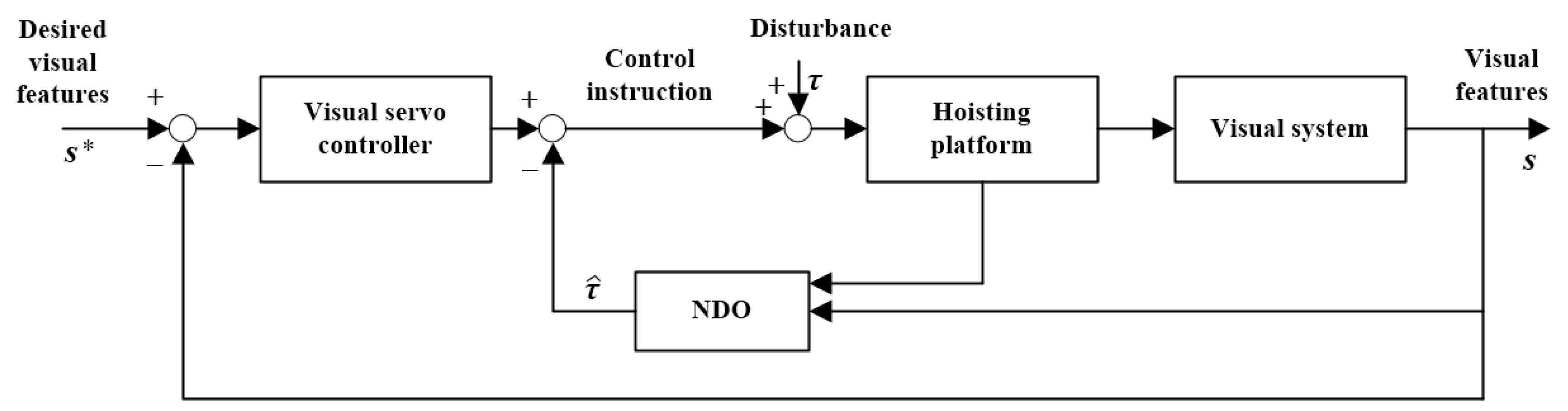
we have the conclusion that $\dot{V}$ is both negative and positive definite and the system is asymptotically stable. The structure of the control loop is shown in Figure 6.

5. Simulations

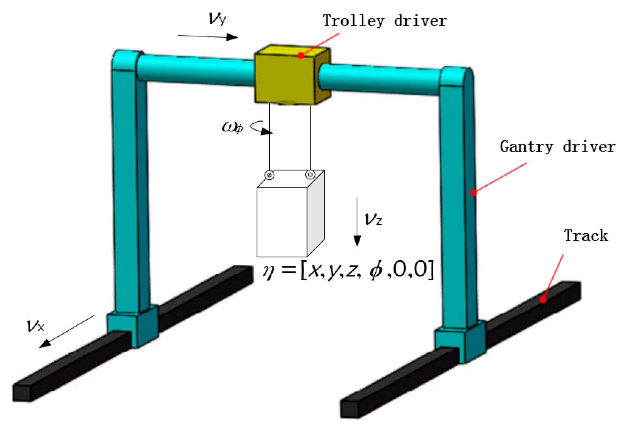
The proposed visual servo positioning method is applied to the simulation platform. Simulations are conducted to investigate the control performance of the proposed controller in the presence of system uncertainties and disturbance.

Consistent with the actual project, we adopt the eye-in-hand style in the simulation platform. To simulate the real camera projection, the controller needs the parameters of the camera, and we use a visual toolbox with the following parameters: focal length 8 mm, imaging pixel frame 1024 × 1024. The intention of this simulation is to drive the manipulator to the desired pose. The system parameters are set as $k_p=diag\left\{0.8,0.8,0.68,0.4,0,0\right\}$, $k_s=diag\left\{0.6,0.6,0.6,0.35,0,0\right\}$, the disturbance term ${\left[5.5,5.5,5.5,0.1,0,0\right]}^{\mathrm{T}}$ is exerted on control quantities. The sampling time is set as t = 10 ms. In the simulation, the delay is not considered, which means that, in the ideal state, the time of visual feature extraction and processing is not calculated, and the visual error curve is smooth. We will take the data sampled as the updated data for subsequent analyses and calculations. In this way, the simulation of hoisting positioning with disturbance is carried out to verify the superiority of the method proposed in this paper.

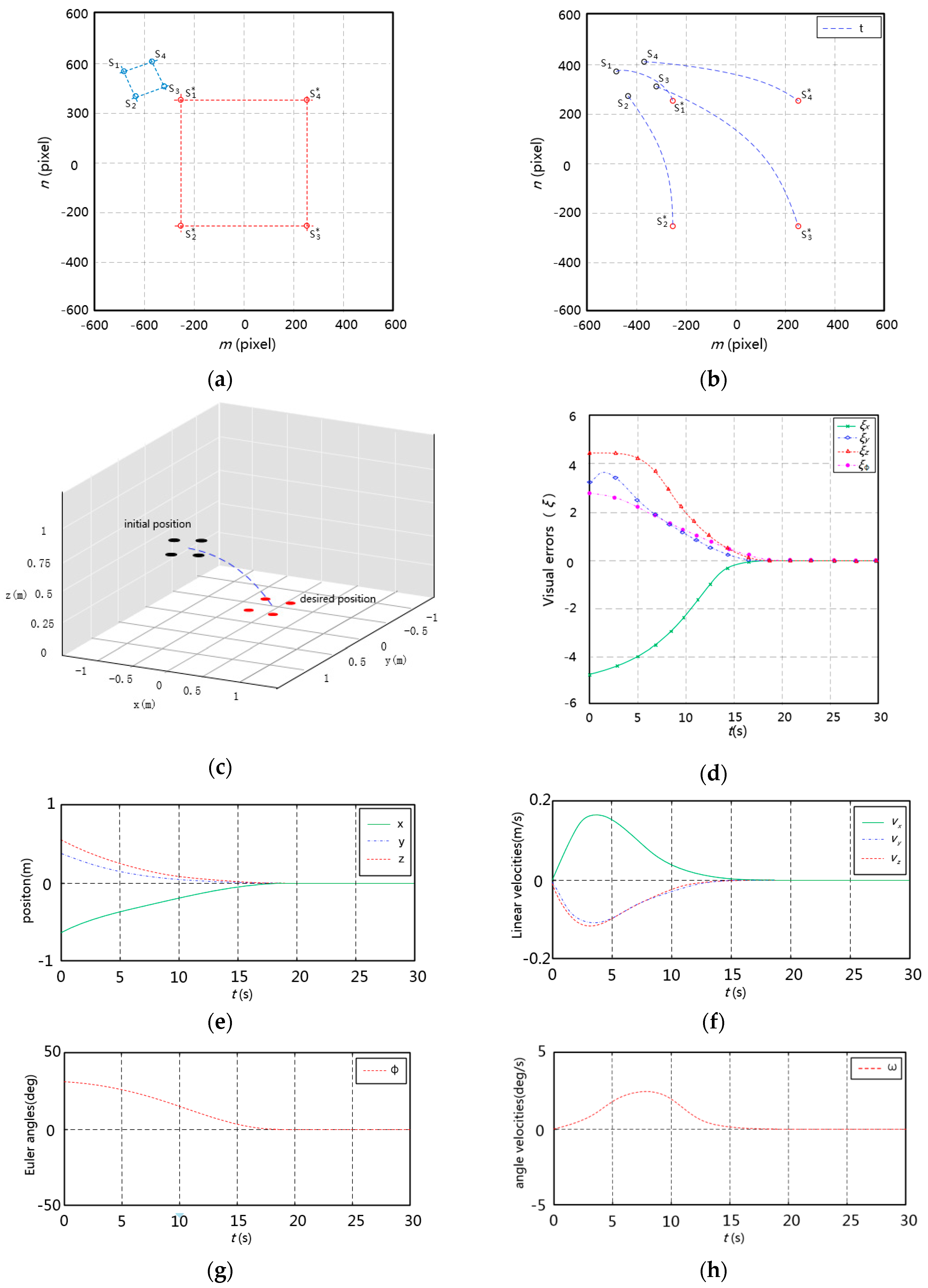
The initial pose of the manipulator is set as ${\left[-0.6,0.4,0.5,\pi /12,0,0\right]}^{\mathrm{T}}$. The initial feature points and the desired feature points in the image plane are shown in Figure 7a; $s_1,s_2,s_3,s_4$ represent the initial points, and $s_1^{\ast },s_2^{\ast },s_3^{\ast },s_4^{\ast }$ represent the desired points. In Figure 7b, the blue dotted lines represent the trajectories of four points; we can see that, although there is a large displacement between the initial position and the desired position, the manipulator can still be driven to the exact position. During the whole motion process, we take the feature center point as the record point to display its trajectory in 3D space, as shown in Figure 7c. The curvature of the simulation curve in three-dimensional space is small, which means that the proposed method can drive the control object to the target position in a shorter path. After the convergence of visual error, it is stable at zero, which shows that our method still has satisfactory accuracy in the presence of uncertainty and disturbance. Although the position curves have tiny tilt angles, the final position converges and stabilizes at zero. In our method, an adaptive sliding mode control algorithm is employed to decrease the influence of external disturbance, and the coefficient of the slide surface is established based on the adaptive gain. Obviously, this can drive the object to the target position smoothly.

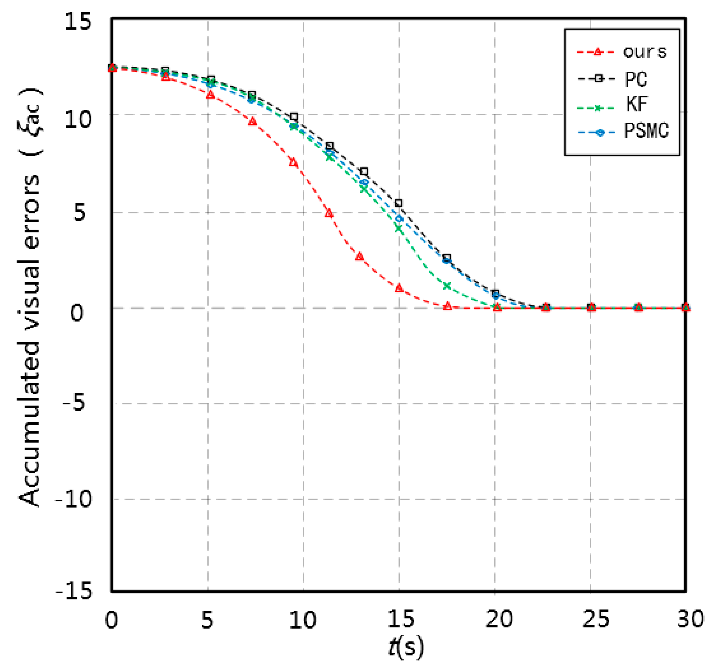
Furthermore, we compare the proposed method with the other methods, including proportional control (PC) visual servo, PSMC visual servo [35] and Kalman Filtering (KF) visual servo [36]. The PSMC visual servo proposes a combination of proportional control with the sliding mode control method. Image moments of circular markers labeled are selected as visual features to control the three translational degrees of freedom (DOFs) of the manipulator. The KF visual servo presents an image-based servo control approach with a Kalman neural network filtering scheme; this uses a neural network to estimate and compensate the errors of Kalman filtering (KF). A computer with Intel Corei5 2.67 GHz CPU, 4 GB RAM is used in this comparison. The diagonal positive definite gain matrix $K_p$ in the PC visual servo is set as the same as our controller; the diagonal positive definite gain matrices $\lambda$, $K_p$, $K_s$ in [35] and the minimum sum squared error (MSE) in [36] are set according to their default values.

The comparison results of the accumulated visual errors are shown in Figure 8. The quantitative results of the specific comparison are listed in

Table 1. Quantitative comparison result.

Method	Convergence Time (s)	Computational Time (ms)	Number of Servo Cycles
ASMCN visual servo (ours)	18.05	150	120
PC visual servo	22.20	149	149
KF visual servo	20.21	157	129
PSMC visual servo	22.15	155	143

. Although the computational time of our method is a little longer than that of the PC visual servo, the ASMCN visual servo (ours) has a better convergence performance. Our method has fewer servo cycles, due to the introduction of a nonlinear disturbance observer and the control law with disturbance compensation.

6. Experiments

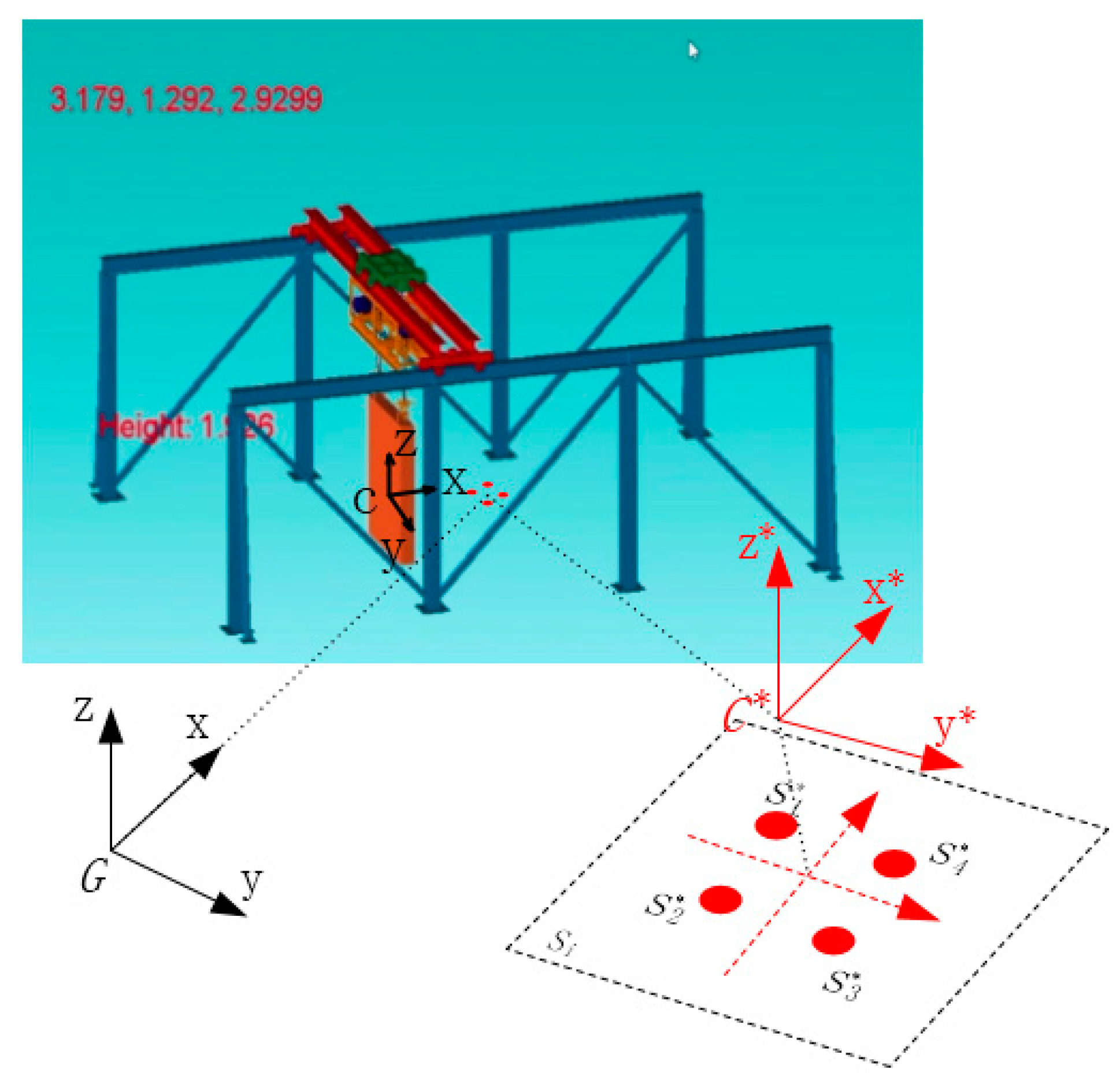
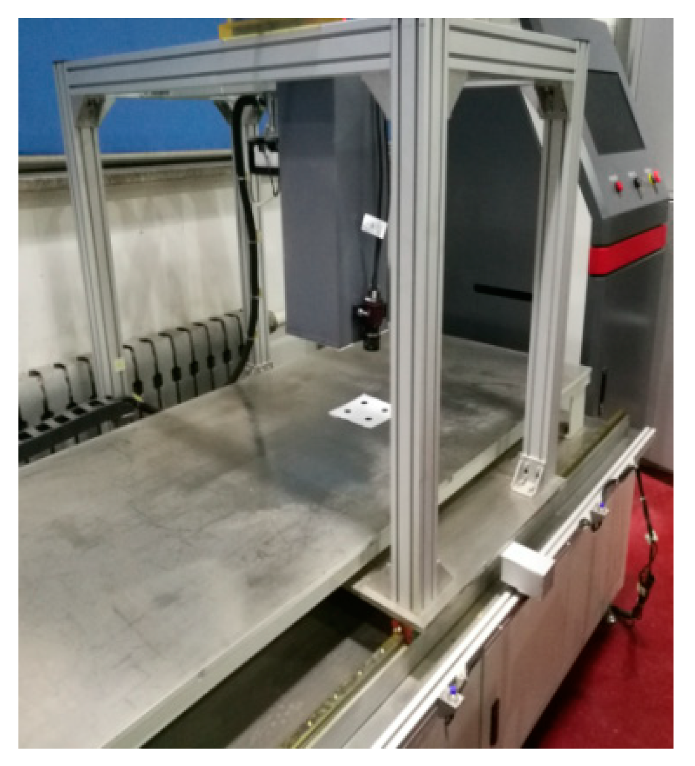
In order to further verify the effectiveness in the actual hoisting work of the control scheme proposed in this paper, we conduct the experimental test using the four-degrees-of-freedom hoisting platform in the laboratory. In the experiment, we drive the heavy-long load component to the target position, and the weight of the load component is up to 300 kg, the overall dimensions of the load component are 0.4 × 0.4 × 1.2 (m) of height, width, and length. For the hoisting platform, the vibration of load and equipment is inevitable when it is hoisting heavy–long load components, which is also consistent with the disturbance condition in the actual hoisting operation. OMRON encoders (E6B2-CWZ6C) connected to the motor are used to measure the velocities. The images are captured by Mako camera (AVT, Germany), using GigE Vision interface and Power-over-Ethernet. Through wired network transmission, we can realize the real-time transmission of visual system and control system. 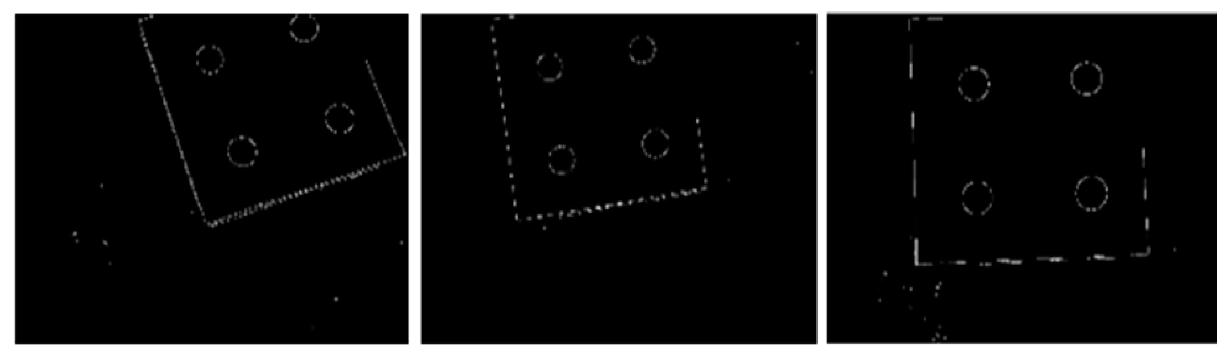The experimental platform is shown in Figure 9. The target is composed of four black origins and a rectangular frame. The Laplacian of the Gaussian algorithm is used to extract the line feature and inner region feature in the image. In the actual condition, the change of light intensity will affect the image quality, and then affect the accuracy of image feature extraction. Therefore, we use adaptive histogram equalization [37] to preprocess the image. Moreover, the feature extraction results of the convergence process are shown in Figure 10.

We carried out two positioning experiments (A and B) by changing the initial position. Firstly, the load component is moved to the target position by the manual system to obtain the desired image and the camera records the characteristic images of different positions. Then, we return to component the initial position, start the automatic control system, and drive the load component to the target position by the proposed scheme. For the IBVS system proposed in this paper, its convergence region is limited due to the nonlinearity and singularity of the desired image to the driving frame. The extracted target points will match to the adjacent target points in the desired image.

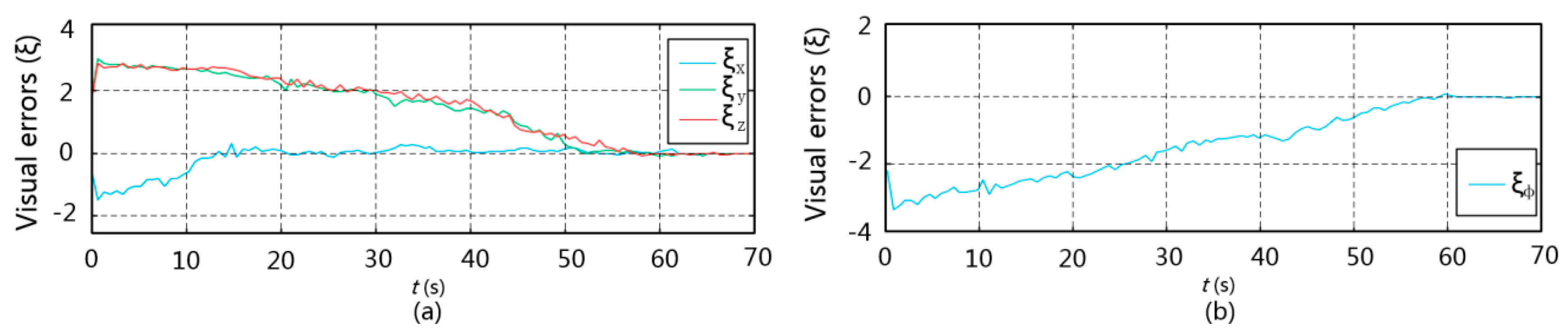
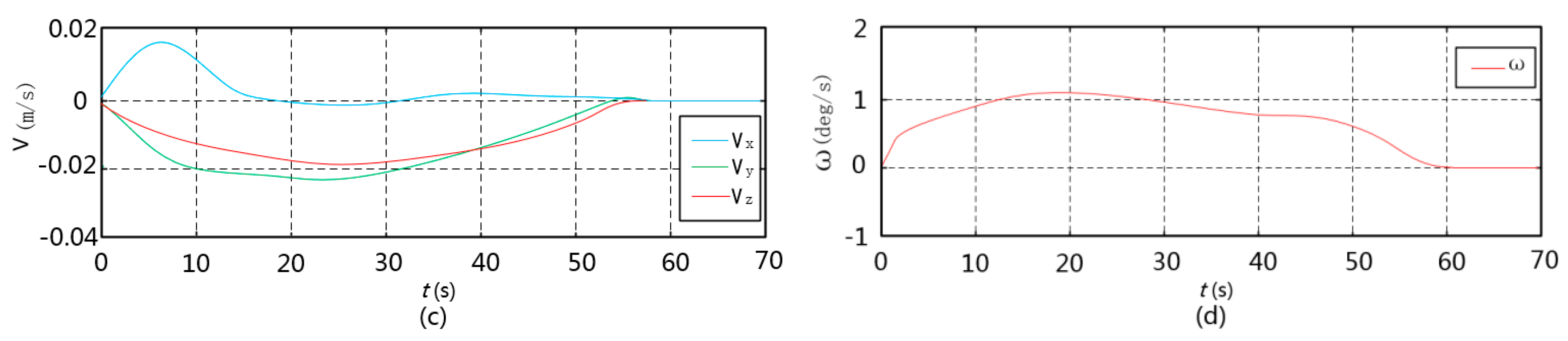
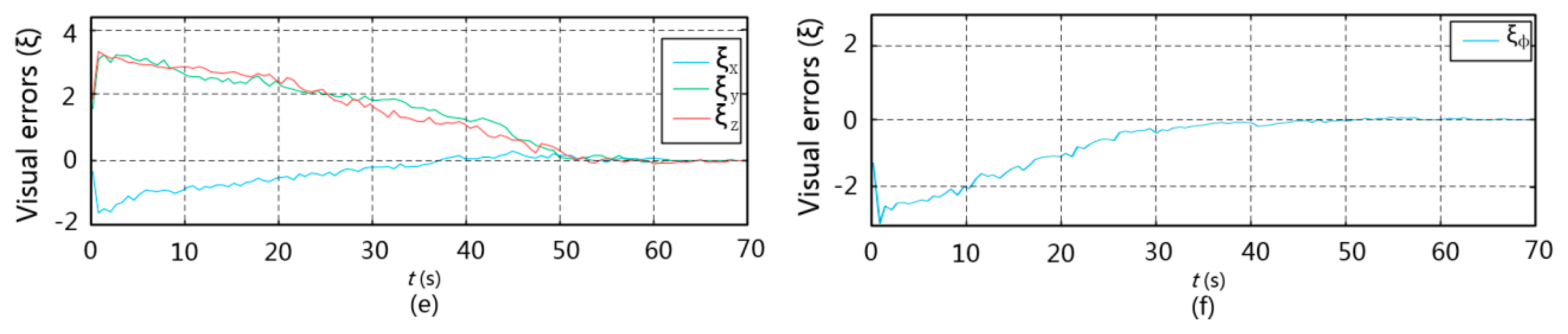
Figure 11a,b depict the visual errors of experiment A, from which we can see that, although the visual error value of the initial position is large, the curves converge quickly and finally reach zero. Obviously, the visual error curve has a zigzag character, which is caused by the disturbance. However, the velocity curve in Figure 12 is relatively smooth, which indicates that the delay of mechanical system is lower and the encoder sensitivity is higher. This also shows that the algorithm in this paper can output stable control signals by adjusting the adaptive gain when the visual signal has a small vibration. 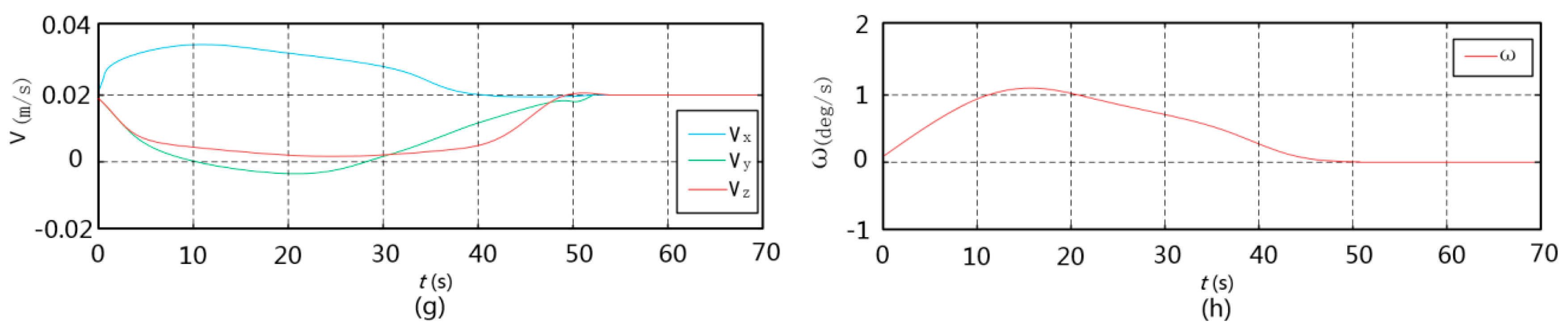As for experiment B, by comparing the (e) and (f) in Figure 13, the visual error of rotation converges earlier than that of the translational direction. The velocity curves in Figure 14 have almost no oscillation effect and can gradually approach zero, which indicates that our method has a robust performance on disturbance suppression and precise positioning.

7. Conclusions

In this paper, we propose a visual servo scheme for hoisting positioning under disturbance condition. Through simulation and experimental verification, we can draw the following conclusions:

(1) We define the visual error by the image error of the feedback signal based on dynamic equations containing disturbance. The relationship between visual error and disturbance is established, which lays a foundation for improving control stability;

(2) In view of the problem that it is difficult to model disturbance terms, a nonlinear disturbance observer is introduced to obtain the equivalent disturbance. On this basis, an adaptive control algorithm with disturbance compensation is proposed to improve the robustness and convergence of the visual servoing scheme;

(3) The results of experiment show that the algorithm in this paper can output stable control signals by adjusting the adaptive gain when the visual signal has a small vibration, and our method shows satisfactory positioning accuracy.

Visual servoing control for hoisting positioning is still a problem worthy of further study, including research on robust uncalibrated visual servoing control and velocity estimation from finite visual features.