Accelerating High-Resolution Seismic Imaging by Using Deep Learning

Abstract

The emerging applications of deep learning in solving geophysical problems have attracted increasing attention. In particular, it is of significance to enhance the computational efficiency of the computationally intensive geophysical algorithms. In this paper, we accelerate deabsorption prestack time migration (QPSTM), which can yield higher-resolution seismic imaging by compensating absorption and correcting dispersion through deep learning. This is implemented by training a neural network with pairs of small-sized patches of the stacked migrated results obtained by conventional PSTM and deabsorption QPSTM and then yielding the high-resolution imaging volume by prediction with the migrated results of conventional PSTM. We use an encoder-decoder network to highlight the features related to high-resolution migrated results in a high-order dimension space. The training data set of small-sized patches not only reduces the required high-resolution migrated result (for instance, only several inline is required) but leads to a fast convergence in training. The proposed deep-learning approach accelerates the high-resolution imaging by more than 100 times. Field data is used to demonstrate the effectiveness of the proposed method.

1. Introduction

Understanding the underground structure is essential to energy exploration, avoiding natural disasters, and studying the evolution of the Earth. Pre-stack time migration (PSTM) has been widely used in academia and industry, mainly because of its robustness against velocity errors. In fact, neither acoustic or elastic approximation can accurately describe the seismic wave propagation in the real Earth, for example, strong attenuation can exist in the weathering layers. However, the conventional PSTM ignores the viscosity of the medium, which leads to the absence of high-frequency components and results in low-resolution migration images. Zhang [1,2] introduced an effective Q approach (QPSTM) to compensate for the attenuated energies, which are crucial for high-resolution imaging. However, in contrast to the conventional PSTM, the QPSTM approach involves performing an additional integral over all the frequencies, which is time consuming and prevents the application of this approach to large-scale problems. To improve the computational efficiency, Xu [3] distributed the heavy workload to graphics processing units (GPUs) and optimized the calculation at the programming level. Although the use of the GPUs is beneficial, the approach remains less efficient for solving realistic problems; for instance, performing a realistic 3D QPSTM can take several months even when using advanced GPU clusters. Consequently, we continue to seek better solutions, and the emerging machine learning algorithms appear to be a promising tool to solve this problem.

The use of artificial intelligence (AI), involving deep learning (DL) [4,5] approaches, has achieved success in many research areas, such as natural language processing [6,7,8], image classification [9,10,11,12,13,14], image super-resolution [15,16,17,18], image retrieval [19,20,21,22], and so on. In addition, geophysicists have attempted to adopt DL to solve particular problems: Jia [23] employed the support vector regression method to solve the missing-data interpolation problem. To perform seismic data interpolation, Wang [24] designed an eight-layer residual learning network based on a convolutional neural network (CNN) [25]. Xiong [26] adopted the widely used classification networks to detect faults from migration images. Qian [27] introduced the deep neural network to extract features from 2D prestack gathers. Yang [28] adapted the DL method to velocity estimation without requiring any prior information. Wang [29] introduced the DL strategy into seismic data interpolation to provide accurately reconstructed dense data. Hu [30] proposed the identification of the first arrivals by using convolution networks. Zhang [31] introduced a regularized elastic full-waveform inversion by using DL. In addition, Hu [32] used a progressive deep transfer learning approach to predict the missing low-frequency components in seismic data.

Considering this background, in this study, an end-to-end high resolution seismic imaging method was developed by exploiting DL to realize an affordable QPSTM. The proposed model is an encoder-decoder framework that performs a detailed feature extraction of the seismic images.

2. Methods

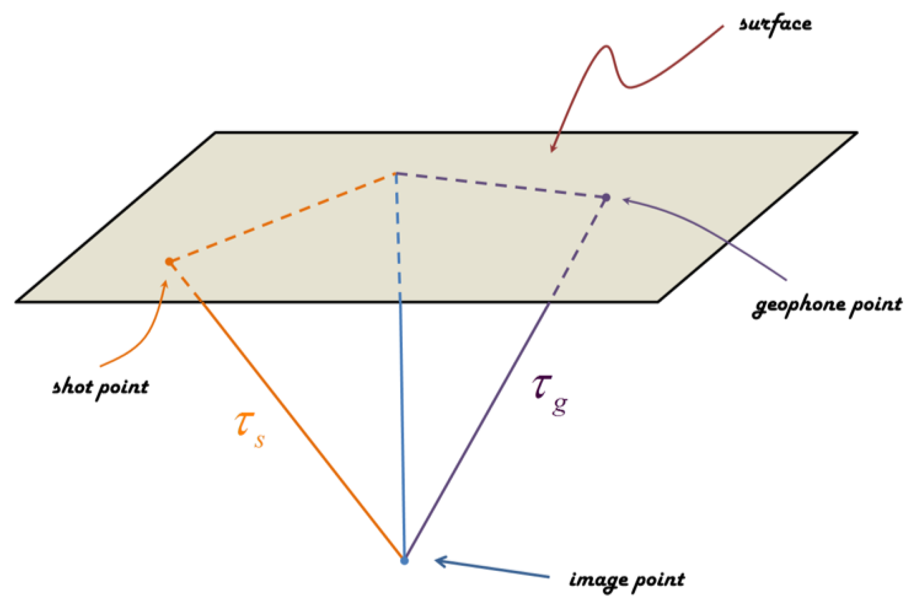
2.1. High-Resolution Imaging Using QPSTM

The QPSTM can be expressed as [1,2],

$$\begin{array}{c}I(x,y,T)={\left(\frac{{\tau }_s}{{\tau }_g}\right)}^2{\int }_{\omega }F\left(\omega \right)e^{-j\frac{\pi }{2}}{e}^{j\omega \left({\tau }_s+{\tau }_g\right)\left(1-\frac{ln\left(\omega /{\omega }_0\right)}{\pi Q_{eff}}\right)}\\ e^{\left(\frac{\omega }{2Q_{eff}}\left({\tau }_s+{\tau }_g\right)\right)}d\omega ,\end{array}$$

(1)

where $I(x,y,T)$ is the image at the horizontal location $(x,y)$ and vertical time-depth T. ${\tau }_s$ and ${\tau }_g$ denote the travel time from the source and the receiver to the imaging point, respectively, as shown in Figure 1. $F\left(\omega \right)$ denotes the seismic traces in the frequency domain. ${\omega }_0$ represents the dominant frequency of the seismic data. $Q_{eff}$ is a factor that represents the intensity of absorption and dispersion of the seismic waves during propagation. This approach is a frequency-domain imaging method as there exists an integral over $\omega$. The frequency components for each imaging point are accumulated, which makes this approach computationally intensive.

To verify the effectiveness of the QPSTM, we tested it on a synthetic marine model. Figure 2 shows the P-wave velocity structures. The upper-shallow layer is a water layer with a velocity of 1500 m/s. The velocity increases with an increase in the depth. In addition, the model includes several faults, and overthrust structures. A Q model with the same size as that of the velocity model was used. We generated the synthetic shot-gathers, taking into account the attenuation and dispersion, by using the modeling method proposed by Hui [33]. Next, the modeled data was migrated by using the conventional PSTM and QPSTM method. The corresponding imaging results are shown in Figure 3 and Figure 4. Sedimentary layers, faults and overthrusts can be clearly observed, which can help analyze the sedimentary relationship better. It is thus concluded that the QPSTM can significantly improve the resolution of the migration image.

However, the computation cost of the QPSTM is larger than that of the conventional PSTM. For example, it takes 115 and 2218 s to calculate the simple 2D profile in Figure 3 and Figure 4, respectively. Even when using GPUs, several months may be required to obtain the high-resolution results for a real 3D field dataset [3]. This prevents the application of this approach to large-scale problems. Furthermore, the low efficiency makes the parameter update more difficult and energy intensive.

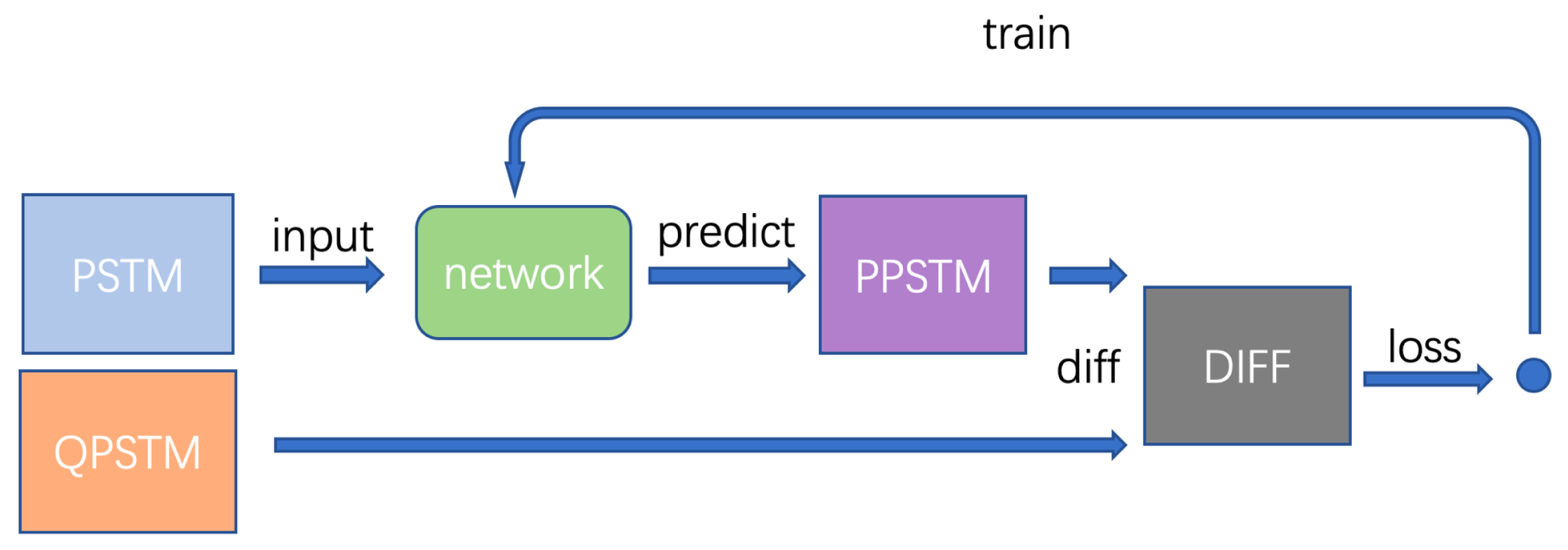
2.2. Network Architecture

To leverage the information within the high-resolution imaging results and enhance the efficiency of the QPSTM, we proposed a CNN network architecture, inspired by Deep Labv3 [34,35] and U-Net [36]. The network was used to map the conventional PSTM results to the high-resolution imaging results. The network has two parts, namely, the encoder and decoder. As shown in Figure 5, the encoder compresses the large-size input, that is, the PSTM migration image, into smaller ones. Additionally, the low-level layer has fewer features than the high-level layers. In other words, in the encoding process, the data dimension becomes smaller and deeper, and the information is transformed from the space domain to the feature domain. The transformations from layer to layer rely on the convolution neutral layer [4,9,37,38] and rectified linear unit (ReLU) activation function [9]. Conversely, in the decoding procedure, illustrated on the right side of Figure 5, the information from the deeper feature map is transformed to the image space by using a transposed-convolution layer [38,39]. The final output layer uses a $1\times 1$ convolutional layer, which represents the high-resolution result patches. This layer is followed by a tanh activation function, for which the actual expected result is $[-1,+1]$. To overcome the spatial-resolution loss, a skip connection is applied between the encoder and decoder directly [36]. The details of each layer are presented in

Table 1. Parameters of each layer.

Layer	Output Shape	Connected to
input-1	(64,128,1)
conv2d-1	(64,128,64)	input-1
conv2d-2	(64,128,64)	conv2d-1
max-pooling2d-1	(32,64,64)	conv2d-2
conv2d-3	(32,64,128)	max-pooling2d-1
conv2d-4	(32,64,128)	conv2d-3
max-pooling2d-2	(16,32,128)	conv2d-4
conv2d-5	(16,32,256)	max-pooling2d-2
conv2d-6	(16,32,256)	conv2d-5
max-pooling2d-3	(8,16,256)	conv2d-6
conv2d-7	(8,16,512)	max-pooling2d-3
conv2d-8	(8,16,512)	conv2d-7
dropout-1	(8,16,512)	conv2d-8
max-pooling2d-4	(4,8,512)	dropout-1
conv2d-9	(4,8,1024)	max-pooling2d-4
conv2d-10	(4,8,1024)	conv2d-9
dropout-2	(4,8,1024)	conv2d-10
up-sampling2d-1	(8,16,1024)	dropout-2
conv2d-11	(8,16,512)	up-sampling2d-1
concatenate-1	(8,16,1024)	dropout-1
		conv2d-11
conv2d-12	(8,16,512)	concatenate-1
conv2d-13	(8,16,512)	conv2d-12
up-sampling2d-2	(16,32,512)	conv2d-13
conv2d-14	(16,32,256)	up-sampling2d-2
concatenate-2	(16,32,512)	conv2d-6
		conv2d-14
conv2d-15	(16,32,256)	concatenate-2
conv2d-16	(16,32,256)	onv2d-15
up-sampling2d-3	(32,64,256)	conv2d-16
conv2d-17	(32,64,128)	p-sampling2d-3
concatenate-3	(32,64,256)	conv2d-4
		conv2d-17
conv2d-18	(32,64,128)	concatenate-3
conv2d-19	(32,64,128)	conv2d-18
up-sampling2d-4	(64,128,128)	conv2d-19
conv2d-20	(64,128,64)	up-sampling2d-4
concatenate-4	(64,128,128)	conv2d-2
		conv2d-20
conv2d-21	(64,128,64)	concatenate-4
conv2d-22	(64,128,64)	conv2d-21
conv2d-23	(64,128,1)	conv2d-22

. Using such an encoder/decoder framework, we can transform the data from one style to another. In particular, the transformation is not a simple pixel-to-pixel mapping but a feature-to-feature mapping in a high-dimension domain.

2.3. End-to-End Learning with Small Patches

In most applications pertaining to computer vision science, the image is treated as a whole feature input [40,41,42,43,44,45]. Consequently, images with different sizes need to be resized or cropped to a fixed size before being fed into the network. Seismic profile mapping involves more features and characteristics than those for computer image processing, for instance, the features corresponding to semantic segmentation and object detection and classification. Furthermore, mapping the conventional PSTM result to a high-resolution migration image requires the subtle modification of the frequency of the network, which is not spatial/area sensitive. In addition, the use of small-size inputs can make the convergence of the network easier in the training stage and more efficient in the prediction stage.

In this study, a relatively small patch size of $64\times 128$ was selected. The dimension 64 was the number of common depth points (CDPs), and the time-depth dimension corresponded to 128 imaging points. The patches are illustrated in Figure 6. It can be noted that diverse patches with different patterns exist: some patches consist of low-frequency components, whereas the others are compounds of high-frequency components. In addition, the dip angle of the structures varies from patch to patch. In the subsequent sections, we describe the generation of the patches from the imaging result and the data pre-processing, specifically for DL.

After the prerequisite processing (e.g., de-noising, static correction for land data, consistent de-convolution, de-multiples for marine data, velocity analysis) of the field seismic data, the 3D migration data volume can be obtained by using the conventional PSTM method. High-resolution imaging using the QPSTM method can be performed for a given imaging line to control the learning procedure. In the actual situation, 20 lines from the work area were considered as the proposal lines. Thereafter, we divided the image result of the proposal lines (including the results of the conventional PSTM and QPSTM) into patches. Specifically, we sampled the patches from the imaging result using a sliding window. In general, the first patch sample was obtained at the left-top (the minimum CDP and minimum time-depth position) of one imaging profile. Next, we moved the window to the right with a fixed step of 32-CDP. After the first row was scanned, we moved the time-depth by a step with 64 time sampling points. After repeating the sampling procedure, the conventional PSTM imaging patches and the corresponding high-resolution imaging patches were obtained. Varying the actual amplitude range from patch to patch was not suitable for training the network; therefore, we scaled the range to $[-1,1]$ by performing amplitude normalization using Equation (2):

$$s(x,t)=\left\{\begin{array}{ccc}\hfill f(x,t)/max& & f(x,t)\ge 0\hfill \\ \hfill -f(x,t)/min& & f(x,t)<0.\hfill \end{array}\right.$$

(2)

Here, $s(x,t)$ is the scaled amplitude of each patch, and $max$ and $min$ denote the positive maximum and negative minimum amplitudes, respectively. $f(x,t)$ denotes the original image patches. When the original data is greater than or equal to 0, $max$ is used as the numerator; otherwise, minus $min$ is divided. After the amplitude balance, the data range of each patch is normalized to $[-1,+1]$. As shown in Figure 7, the $PSTM$ block represents the balanced conventional PSTM result patches, and the $QPSTM$ block denotes the balanced QPSTM patches. The $PSTM$ patch was fed to the network as the input. After the feature encoding and decoding, the network predicted the output, denoted as $PPSTM$ in the figure. It should be noted that the $PPSTM$ had the same size as that of the $PSTM$ and $QPSTM$ patches. In the training phase, the difference (shown as $DIFF$ in figure) was obtained element-wise in the patch. Furthermore, we evaluated the loss, a scalar that represents the difference between the predicted and the ground truth result, by using the mean absolute error (MAE), which is defined as

$$Loss=\sum _{ix=1}^{nx}\sum _{it=1}^{nt}|p(x,t)-q(x,t)|,$$

(3)

where $p(x,t)$ is the predicted patch with the filtering effect of the network from the original PSTM imaging patch, and $q(x,t)$ represents the QPSTM imaging patches. In this case, we use the MAE instead of the mean square error (MSE) as the loss function, because the MSE can smear the different phases of the seismic events, thereby mitigating the gradient difference. In a DL framework, the obtained loss is back-propagated to the network to update the network’s hyper-parameters and make the network more suitable for the training data set. Among the several optimization methods that can be used to train the network, in this study, the widely used Adam optimizer [46] was employed owing to its computational efficiency and ability to obtain the adaptive estimates of the lower-order moments.

The prediction phase is easier to understand than the training procedure. Figure 7 illustrates the prediction and training phases together. In the prediction phase, only the PSTM patches are input to a well-trained network. In our framework, the training is conducted, and the scale is applied for every patch (as defined in Formula (2)). However, the objective is to attain the high-resolution images. To this end, in the prediction phase, when scaling the PSTM patch, we memorize $max,min$ at the time. After feeding the patches into the network and obtaining the predicted patches, $max,min$ is eliminated from these patches. Consequently, each predicted patch has a comparable energy intensity and a constant scale factor. In addition, Figure 5 and Table 1 indicate that the last layer of the network is an up-sampling convolution layer. It is difficult to reduce the boundary artifacts induced by the size extension. To suppress these artifacts, we retain only the inner half of the predicted patch. In particular, we predict the patch with a size of $64\times 128$ pixels; however, we only select the inner $32\times 64$ pixels as the meaningful result. We choose the overlapped patches as the input and obtain the overlapped output. After cropping and merging, the final result can be obtained.

In the end-to-end learning, the framework is mapped from one image profile to another image profile with some features emphasized. The features are automatically learned from the given data during the training process. The feature extraction and representation are hidden in the network’s training/prediction procedure. In computer vision science, the image is treated as a whole input; however, in geophysics, especially in exploration seismology, the image is characterized by high complexity and diversity. Therefore, we proposed the use of a small patch-to-patch learning method, which is also an image-to-image model. In all the aspects, we achieved end-to-end learning.

2.4. Data Set

We train and validate the proposed method with real 3D field data. The field data set includes nearly 3000 shots, with a shot interval of 12.5 m, and receiver interval of 12.5 m. Each shot has 2688 receivers. The time sampling interval is 2 ms. The complete fold time is 200. After the pre-processing, the volume is migrated using the conventional PSTM method. Four lines from the migrated volume are used as the network input data. Simultaneously, high-resolution imaging corresponding to these four lines is performed, and the results are used as the predication target output. Three of the four lines are used to train and test the network. The remaining line is used to demonstrate the effectiveness of the proposed method. Under the considered measurement configuration, the output profile of the remaining line involves 601-CDPs and 1001 time samples. All the profiles are divided into small patches sized $64\times 128$. For the three profiles, we obtain 3564 samples in total. To overcome the over-fitting problem [47] and improve the generalization ability, each patch is flipped up/down and left/right and rotated by ${90}^{\circ }$. Consequently, we obtain 14,256 input patches and the corresponding high-resolution patches. From these patches, we select $80\%$ randomly as the training data set, and the remaining $20\%$ of the patches are used as the validation samples.

3. Results

The end-to-end high-resolution imaging method was applied for a real field data set. Additionally, the synthetic Ricker wavelet plane was input into the learned model to illustrate the model learning. In addition, the spectrum of the original and learned high-resolution imaging was compared.

Figure 8 shows the input patches and corresponding learning targets (high-resolution imaging using QPSTM) obtained from these samples. It can be noted that in the conventional PSTM imaging patches, the seismic event is absorbed, with insufficient resolution. However, the corresponding high-resolution imaging patches have more detailed information. These patches are fed into the network, and the network is trained using the TensorFlow program [39] by employing a GPU. The loss curve for the training data and validation data is obtained, as shown in Figure 9. The horizontal axis denotes the training epochs, which represents the number of times that the samples are fed to the network. The vertical axis represents the loss, in particular, the MAE, which indicates the discrepancy between the predicted output and the actual QPSTM imaging result. As the epoch increases from 1 to 25, both the training loss and validation loss decrease dramatically, which means that the network converges to a more fitting state for the provided data. As the epoch moves beyond 25, the loss decreases; however, the speed reduces, indicating that the network is in a fine tuning state. Finally, the validation loss is more than the training loss, accompanied by vibration. This phenomenon indicates that the network model has achieved its state-of-the-art state, and more training may lead to over-fitting or instability. Therefore, we terminate training just before this point, and it takes approximately 4 h to train the whole network by using a TiTan XP GPU.

To validate the proposed approach and illustrate the network learning, a Ricker wavelet compounded plane with a dominated frequency at 30 Hz is used. This Ricker wavelet patch is fed into the network model, and the predicted output of the network is obtained. As shown in Figure 10, the trained model can improve the dominated frequency from 30 Hz to approximately 40 Hz, and the phase is corrected as expected. The synthetics indicate that the model learned the ability to improve the resolution and correct the phase, as described previously using Formula (1).

For further evaluation, a prediction is performed using the patches that the network does not encounter in the training stage. The predicted patches and the ground truth high-resolution imaging result that migrated with the QPSTM are shown in Figure 11. It can be observed that the predicted patches are almost the same as the ground truth patches, which indicate that the network has a high generalization ability.

To realize end-to-end learning, the predicted patches are combined into one fully size seismic imaging profile by using the overlapped sliding window method described in the Methods section and performed energy balancing as described in Formula (2). Finally, the predicted profile is obtained, as shown in Figure 12. For comparison, we use the conventional imaging result obtained using the PSTM (shown in Figure 13) and the imaging profile result obtained using the high-resolution image method (shown in Figure 14). It is obvious that the proposed method can achieve the same imaging effect as the high-resolution imaging method, which requires a large computation time. Both the methods considerably improve the resolution and show sufficiently detailed information of the structure. To intuitively illustrate the improvement, the spectra of the three profiles are compared, as shown in Figure 15. The frequency when using the learning method improved by approximately 16 Hz at the high-frequency end at −20 dB, compared with that for the conventional PSTM result. Both the learned network and the QPSTM exhibit a comparable performance in terms of the frequency improvement.

A total of 304 patches exist in the predicted QPSTM result, as shown in Figure 14. The prediction of each patch by the trained CNN requires approximately 10 ms when using one TITAN Xp GPU, which means that computing the profile (1001 (vertical) × 601 (inline) samples) shown in Figure 14 requires only 3 s. In contrast, more than 32 h are required to compute this profile when using the QPSTM method with one TITAN Xp GPU. In fact, we need to compute 437 profiles for this field data totally. In detail, with the deep learning method, we need to prepare three QPSTM images used for the network as the training samples, which is called data generation cost and takes about 96 h. It takes about 4 h to train the network to a fine state with these samples. The prediction process, which is the procedure to calculate the 437 images by feeding small-patches into the network, takes 0.4 h. As shown in

Table 2. Comparison of the deep learning method and QPSTM method.

	Deep Learning Method (hour)	QPSTM Method (hour)
Computing Resource	One TITAN XP GPU	One TITAN XP GPU
Computing Process	Data Generation (96 h) Training Process (4 h) Prediction Process (0.4 h)	32 h * Profile Number (437)
Total Time	100.4 h	13,984 h
Speedup Ratio	139

, it takes 100.4 h for the deep learning method to calculate these results with one GPU, while the QPSTM method takes 13,984 h to get similar results. The computing efficiency ultimately improved more than 100 times. Hence, the efficiency of the high-resolution imaging procedure combined with the end-to-end method is significantly improved compared with that of the QPSTM method.

4. Conclusions

The encoder-decoder network can learn the high-resolution patterns hidden in the computationally intensive QPSTM migration images. The proposed high-resolution end-to-end seismic imaging method can predict images as well as those calculated using the QPSTM. The use of small patches instead of the full image in the training and prediction helps improve the efficiency and the generalization ability of the network considerably. A real data set and synthetic data are used to validate the effectiveness of the proposed method. End-to-end learning can hide the inherent transformation of information. Deep learning can not only perform high-dimensional data feature extraction but can also be used to accelerate scientific calculations with complex logic. It may be valuable to extend this idea to other related scientific domains.

References

1. Zhang, J.; Wu, J.; Li, X. Compensation for absorption and dispersion in prestack migration: An effective Q approach. Geophysics 2012, 78, S1–S14. [Google Scholar] [CrossRef]
2. Zhang, J.; Li, Z.; Liu, L.; Wang, J.; Xu, J. High-resolution imaging: An approach by incorporating stationary-phase implementation into deabsorption prestack time migration. Geophysics 2016, 81, S317–S331. [Google Scholar] [CrossRef]
3. Xu, J.; Liu, W.; Wang, J.; Liu, L.; Zhang, J. An efficient implementation of 3D high-resolution imaging for large-scale seismic data with GPU/CPU heterogeneous parallel computing. Comput. Geosci. 2018, 111, 272–282. [Google Scholar] [CrossRef]
4. LeCun, Y.; Bengio, Y.; Hinton, G. Deep learning. Nature 2015, 521, 436. [Google Scholar] [CrossRef]
5. Goodfellow, I.; Bengio, Y.; Courville, A. Deep Learning; MIT Press: Cambridge, MA, USA, 2016. [Google Scholar]
6. Kalchbrenner, N.; Grefenstette, E.; Blunsom, P. A convolutional neural network for modelling sentences. arXiv 2014, arXiv:1404.2188. [Google Scholar]
7. Tai, K.S.; Socher, R.; Manning, C.D. Improved semantic representations from tree-structured long short-term memory networks. arXiv 2015, arXiv:1503.00075. [Google Scholar]
8. Devlin, J.; Chang, M.W.; Lee, K.; Toutanova, K. Bert: Pre-training of deep bidirectional transformers for language understanding. arXiv 2018, arXiv:1810.04805. [Google Scholar]
9. Krizhevsky, A.; Sutskever, I.; Hinton, G.E. Imagenet classification with deep convolutional neural networks. In Proceedings of the Advances in Neural Information Processing Systems, Lake Tahoe, NV, USA, 3–6 December 2012; pp. 1097–1105. [Google Scholar]
10. Simonyan, K.; Zisserman, A. Very deep convolutional networks for large-scale image recognition. arXiv 2014, arXiv:1409.1556. [Google Scholar]
11. Szegedy, C.; Liu, W.; Jia, Y.; Sermanet, P.; Reed, S.; Anguelov, D.; Erhan, D.; Vanhoucke, V.; Rabinovich, A. Going deeper with convolutions. In Proceedings of the IEEE Conference on Computer Vision and Pattern Recognition, Boston, MA, USA, 7–12 June 2015; pp. 1–9. [Google Scholar]
12. He, K.; Zhang, X.; Ren, S.; Sun, J. Deep residual learning for image recognition. In Proceedings of the IEEE Conference on Computer Vision and Pattern Recognition, Las Vegas, NV, USA, 26 June–1 July 2016; pp. 770–778. [Google Scholar]
13. Deng, C.; Xue, Y.; Liu, X.; Li, C.; Tao, D. Active transfer learning network: A unified deep joint spectral–spatial feature learning model for hyperspectral image classification. IEEE Trans. Geosci. Remote. Sens. 2018, 57, 1741–1754. [Google Scholar] [CrossRef] [Green Version]
14. Ren, S.; He, K.; Girshick, R.; Sun, J. Faster r-cnn: Towards real-time object detection with region proposal networks. In Proceedings of the Advances in Neural Information Processing Systems, Montreal, QC, Canada, 7–12 December 2015; pp. 91–99. [Google Scholar]
15. Ledig, C.; Theis, L.; Huszár, F.; Caballero, J.; Cunningham, A.; Acosta, A.; Aitken, A.; Tejani, A.; Totz, J.; Wang, Z.; et al. Photo-realistic single image super-resolution using a generative adversarial network. In Proceedings of the IEEE Conference on Computer Vision and Pattern Recognition, Honolulu, HI, USA, 21–26 July 2017; pp. 4681–4690. [Google Scholar]
16. Lai, W.S.; Huang, J.B.; Ahuja, N.; Yang, M.H. Deep laplacian pyramid networks for fast and accurate super-resolution. In Proceedings of the IEEE Conference on Computer Vision and Pattern Recognition, Honolulu, HI, USA, 21–26 July 2017; pp. 624–632. [Google Scholar]
17. Fan, X.; Yang, Y.; Deng, C.; Xu, J.; Gao, X. Compressed multi-scale feature fusion network for single image super-resolution. Signal Process. 2018, 146, 50–60. [Google Scholar] [CrossRef]
18. Ulyanov, D.; Vedaldi, A.; Lempitsky, V. Deep image prior. In Proceedings of the IEEE Conference on Computer Vision and Pattern Recognition, Salt Lake City, UT, USA, 18–22 June 2018; pp. 9446–9454. [Google Scholar]
19. Lin, K.; Yang, H.F.; Hsiao, J.H.; Chen, C.S. Deep learning of binary hash codes for fast image retrieval. In Proceedings of the IEEE Conference on Computer Vision and Pattern Recognition Workshops, Boston, MA, USA, 7–12 June 2015; pp. 27–35. [Google Scholar]
20. Li, W.J.; Wang, S.; Kang, W.C. Feature learning based deep supervised hashing with pairwise labels. arXiv 2015, arXiv:1511.03855. [Google Scholar]
21. Liu, H.; Wang, R.; Shan, S.; Chen, X. Deep supervised hashing for fast image retrieval. In Proceedings of the IEEE Conference on Computer Vision and Pattern Recognition, Las Vegas, NV, USA, 26 June–1 July 2016; pp. 2064–2072. [Google Scholar]
22. Deng, C.; Yang, E.; Liu, T.; Tao, D. Two-stream deep hashing with class-specific centers for supervised image search. IEEE Trans. Neural Netw. Learn. Syst. 2019. [Google Scholar] [CrossRef]
23. Jia, Y.; Ma, J. What can machine learning do for seismic data processing? An interpolation application. Geophysics 2017, 82, V163–V177. [Google Scholar] [CrossRef]
24. Wang, B.F.; Zhang, N.; Lu, W.K.; Zhang, P.; Geng, J.H. Seismic Data Interpolation Using Deep Learning Based Residual Networks. Eur. Assoc. Geosci. Eng. 2018, 1, 2214–4609. [Google Scholar]
25. LeCun, Y.; Kavukcuoglu, K.; Farabet, C. Convolutional networks and applications in vision. In Proceedings of the IEEE International Symposium on Circuits and Systems, Paris, France, 30 May–2 June 2010; pp. 253–256. [Google Scholar]
26. Xiong, W.; Ji, X.; Ma, Y.; Wang, Y.; AlBinHassan, N.M.; Ali, M.N.; Luo, Y. Seismic fault detection with convolutional neural network. Geophysics 2018, 83, O97–O103. [Google Scholar] [CrossRef]
27. Qian, F.; Yin, M.; Liu, X.Y.; Wang, Y.J.; Lu, C.; Hu, G.M. Unsupervised seismic facies analysis via deep convolutional autoencoders. Geophysics 2018, 83, A39–A43. [Google Scholar] [CrossRef]
28. Yang, F.; Ma, J. Deep-learning inversion: A next generation seismic velocity-model building method. Geophysics 2019, 84, 1–133. [Google Scholar] [CrossRef] [Green Version]
29. Wang, B.; Zhang, N.; Lu, W.; Wang, J. Deep-learning-based seismic data interpolation: A preliminary result. Geophysics 2019, 84, V11–V20. [Google Scholar] [CrossRef]
30. Hu, L.; Zheng, X.; Duan, Y.; Yan, X.; Hu, Y.; Zhang, X. First-arrival picking with a U-net convolutional network. Geophysics 2019, 84, U45–U57. [Google Scholar] [CrossRef]
31. Zhang, Z.d.; Alkhalifah, T. Regularized elastic full waveform inversion using deep learning. Geophysics 2019, 84, R741–R751. [Google Scholar] [CrossRef]
32. Hu, W.; Jin, Y.; Wu, X.; Chen, J. A progressive deep transfer learning approach to cycle-skipping mitigation in FWI. In SEG Technical Program Expanded Abstracts 2019; Society of Exploration Geophysicists: Tulsa, OK, USA, 2019; pp. 2348–2352. [Google Scholar]
33. Dou, H.; Zhang, J. An irregular grid method for acoustic modeling in inhomogeneous viscoelastic medium. Chin. J.-Geophys.-Chin. Ed. 2016, 59, 4212–4222. [Google Scholar]
34. Chen, L.C.; Papandreou, G.; Schroff, F.; Adam, H. Rethinking Atrous Convolution for Semantic Image Segmentation. arXiv 2017, arXiv:1706.05587v3. [Google Scholar]
35. Chen, L.C.; Zhu, Y.; Papandreou, G.; Schroff, F.; Adam, H. Encoder-decoder with atrous separable convolution for semantic image segmentation. In Proceedings of the European Conference on Computer Vision (ECCV), Munich, Germany, 8–14 September 2018; pp. 801–818. [Google Scholar]
36. Ronneberger, O.; Fischer, P.; Brox, T. U-net: Convolutional networks for biomedical image segmentation. In Proceedings of the International Conference on Medical Image Computing and Computer-Assisted Intervention, Munich, Germany, 5–9 October 2015; Springer: Cham, Switzerland, 2015; pp. 234–241. [Google Scholar]
37. LeCun, Y.; Bengio, Y. Convolutional networks for images, speech, and time series. In The Handbook of Brain Theory and Neural Networks; ACM: New York, NY, USA, 1995; Volume 3361. [Google Scholar]
38. Dumoulin, V.; Visin, F. A guide to convolution arithmetic for deep learning. arXiv 2016, arXiv:1603.07285. [Google Scholar]
39. Abadi, M.; Agarwal, A.; Barham, P.; Brevdo, E.; Chen, Z.; Citro, C.; Corrado, G.S.; Davis, A.; Dean, J.; Devin, M.; et al. TensorFlow: Large-Scale Machine Learning on Heterogeneous Systems. 2015. Software. Available online: tensorflow.org (accessed on 3 April 2020).
40. Hariharan, B.; Arbeláez, P.; Girshick, R.; Malik, J. Simultaneous detection and segmentation. In Proceedings of the European Conference on Computer Vision, Zurich, Switzerland, 6–12 September 2014; Springer: Berlin, Germany, 2014; pp. 297–312. [Google Scholar]
41. Long, J.; Shelhamer, E.; Darrell, T. Fully convolutional networks for semantic segmentation. In Proceedings of the IEEE Conference on Computer Vision and Pattern Recognition, Boston, MA, USA, 7–12 June 2015; pp. 3431–3440. [Google Scholar]
42. Hariharan, B.; Arbeláez, P.; Girshick, R.; Malik, J. Hypercolumns for object segmentation and fine-grained localization. In Proceedings of the IEEE Conference on Computer Vision and Pattern Recognition, Boston, MA, USA, 7–12 June 2015; pp. 447–456. [Google Scholar]
43. Badrinarayanan, V.; Kendall, A.; Cipolla, R. Segnet: A deep convolutional encoder-decoder architecture for image segmentation. IEEE Trans. Pattern Anal. Mach. Intell. 2017, 39, 2481–2495. [Google Scholar] [CrossRef] [PubMed]
44. He, K.; Gkioxari, G.; Dollár, P.; Girshick, R. Mask r-cnn. In Proceedings of the IEEE International Conference on Computer Vision, Venice, Italy, 22–29 October 2017; pp. 2961–2969. [Google Scholar]
45. Chen, L.C.; Papandreou, G.; Kokkinos, I.; Murphy, K.; Yuille, A.L. Deeplab: Semantic image segmentation with deep convolutional nets, atrous convolution, and fully connected crfs. IEEE Trans. Pattern Anal. Mach. Intell. 2017, 40, 834–848. [Google Scholar] [CrossRef]
46. Kingma, D.P.; Ba, J. Adam: A method for stochastic optimization. arXiv 2014, arXiv:1412.6980. [Google Scholar]
47. Tetko, I.V.; Livingstone, D.J.; Luik, A.I. Neural network studies. 1. Comparison of overfitting and overtraining. J. Chem. Inf. Comput. Sci. 1995, 35, 826–833. [Google Scholar] [CrossRef]
Sample Availability: Data associated with this research is confidential and the source code is available after the paper has been published online. You can get the source code from https://github.com/reed-lau/migration-migration.git.
Figure 1. Imaging principle of the deabsorption prestack time migration (QPSTM). The shot point is the position where the seismic signal is generated and the geophone point is the position where the signal is received, and the image point is the underground position where the structure is studied. By calculating the travel time between the source-and-receiver pair, τ s and τ g can be obtained. Next, the compensation effect resulting from the Q factor along the wave-path in the frequency domain with an effective Q is determined to achieve the energy-compensated imaging result.
Applsci 10 02502 g001
Figure 2. Synthetic marine velocity model. The velocity model consists of a water layer and several sedimentary layers, with values varying from 1500 to 4000 m/s. The viscous acoustic seismic record was modeled to test the effectiveness of the QPSTM with a same size Q model (not shown here).
Applsci 10 02502 g002
Figure 3. Conventional pre-stack time migration (PSTM) image. The migration image has a relatively lower resolution owing to the energy attenuation and phase distortion.
Applsci 10 02502 g003
Figure 4. QPSTM image. After compensating the energy loss and correcting the phase distortion, the resolution of the image is improved. The fault planes can be clearly seen.
Applsci 10 02502 g004
Figure 5. Schematic of the network structure. The network structure consists of 23 conventional layers. The input layer involves the patches of the PSTM migration images, and the output layer involves the corresponding high-resolution versions of the image (obtained using the QPSTM). The network is not entirely symmetric. In the encoding and decoding phases, the layers’ size is transformed from 64 × 128 × 1 to 4 × 8 × 1024 and from 4 × 8 × 1024 to 64 × 128 × 1 , respectively. The activation function of the encoder and decoder layers is the ReLU. The activation function of the layer before the output is t a n h because the co-domain of the ReLU is [ 0 , + ] , and the actual expected result is [ 1 , + 1 ] . The arrow line between the encoder and decoder layers is the skip connection, which maintains the spatial resolution and positional information and ensures that the feature maps from the up-sampling are more elaborate. Moreover, the introduction of the skip connection makes the network less sensitive to a new data set and ensures that the network has a stronger generalization ability.
Applsci 10 02502 g005
Figure 6. Input patches for training the network. Instead of the full image, small patches are used as the network input. Small images require small networks, which involve fewer parameters to tune and can easily converge in training. Furthermore, small networks have a higher generalization capacity. In addition, small patches cover various features, such as frequency appearance and dip angles. Finally, a large number of training samples can be easily generated using small patches, which is critical for DL applications.
Applsci 10 02502 g006
Figure 7. Network workflow for training and prediction. In the training phase, the patches of the PSTM images are fed into the network and the predicted output is determined. Thereafter, the difference between the prediction patches and the actual migration patches obtained using the QPSTM is calculated, and the loss error is back-propagated to update the network parameters to make it more suitable for the training samples. After training for many epochs, the network converges to a fine state, which can be used to predict unseen patches. In the prediction phase, using the well-trained network and the PSTM patch as the input, we can predict the output patch with a high-resolution feature.
Applsci 10 02502 g007
Figure 8. PSTM patches and the corresponding QPSTM patches used for network training. Panel (a) shows the four input patches, whereas panel (b) shows the corresponding learning targets (high-resolution imaging using QPSTM) from the 14,256 samples. It can be observed that the seismic events are absorbed with insufficient resolution in the conventional PSTM imaging patches, whereas the corresponding high-resolution imaging patches have more detailed information.
Applsci 10 02502 g008
Figure 9. Training loss and validation loss in the training process. After approximately 100 epochs, the model loss remains largely constant, and the training process can be stopped at this point.
Applsci 10 02502 g009
Figure 10. Panel (a) shows the ricker wavelet, whereas panel (b) shows the corresponding predicted result using the trained convolutional neural network (CNN). The black lines in panel (a,b) represent the respective waveforms. The red line and blue line in panel (c) represent the spectrums of the ricker wavelet and its predicted result, respectively. The trained model can improve the dominated frequency of the ricker wavelet from 30 Hz to approximately 40 Hz. In addition, the phase is corrected, as expected.
Applsci 10 02502 g010
Figure 11. True QPSTM patches and patches for unseen data, predicted using the network. Patches in panel (a) represent the input of the network. The predicted patches (shown in panel (b)) are almost the same as the true patches (panel (c)), which indicates that the network has a high generalization ability.
Applsci 10 02502 g011
Figure 12. Predicted image using the proposed method. The proposed method can achieve the same imaging effect as that of the high-resolution imaging method, which requires a large computation time. Both the methods considerably improve the resolution and reflect detailed information of the structure.
Applsci 10 02502 g012
Figure 13. Conventional PSTM image.
Applsci 10 02502 g013
Figure 14. True high-resolution image.
Applsci 10 02502 g014
Figure 15. Comparing the spectra of the ground truth QPSTM and predicted QPSTM. Using the learning method, the frequency improved by approximately 16 Hz at the high-frequency end at −20 dB compared with that of the conventional PSTM. The learned method and QPSTM exhibited comparable performances in terms of the frequency improvement.
Applsci 10 02502 g015