An Automated End-to-End Side Channel Analysis Based on Probabilistic Model

Abstract

In this paper, we propose a new automated way to find out the secret exponent from a single power trace. We segment the power trace into subsignals that are directly related to recovery of the secret exponent. The proposed approach does not need the reference window to slide, templates nor correlation coefficients compared to previous manners. Our method detects change points in the power trace to explore the locations of the operations and is robust to unexpected noise addition. We first model the change point detection problem to catch the subsignals irrelevant to the secret and solve this problem with Markov Chain Monte Carlo (MCMC) which gives a global optimal solution. After separating the relevant and irrelevant parts in signal, we extract features from the segments and group segments into clusters to find the key exponent. Using single power trace indicates the weakest power level of attacker where there is a very slight chance of acquiring as many power traces as needed for breaking the key. We empirically show the improvement in accuracy even with presence of high level of noise.

1. Introduction

Many Side Channel Analysis attacks have succeeded in breaking the secret keys analyzing power trace(s) generated from devices. However, there are many assumptions and limitations on these attacks. Some of them exploit as many power traces as needed to recover secrets. In addition, others have proposed methods to recover secrets from overall power trace(s) but not their exact location on the power trace from which each bit of secrets have been recovered.

One of the well known approaches is to find the reference window and apply a peak detecting algorithm [1,2]. However, the success of this approach heavily depends on the selection of a “good” reference window and the performance of peak detecting algorithms since we cannot search for all the windows in polynomial time. Therefore we need an automated approach that is feasible in polynomial time and does not require human intervention to succeed. Side channel analysis with machine learning has gained much interest [3,4,5,6].

Our work suggests a new approach to finding keys in a Bayesian approach. Our contributions on Side channel analysis and signal processing are as follows:

• We exploit only one single power trace and recover the secret.
• We suggest the methods to compute the probability of locations from which the secret came and find out global optimal solutions in a Monte Carlo approach.
• We suggest the methodology that is more robust than ad-hoc attacks in the presence of noise.

In correlation analysis [2,7,8,9,10,11], a set of power traces is used to find a correlation between the power trace and the key guess. Our method assumes weaker power of an attacker where a chance of acquiring more than one power trace is slight. Analyses with clustering methods [12,13,14] are researched. Recently, horizontal attacks [7] have been succeeding with clustering algorithms [15,16]. These attacks exploiting clustering algorithms and horizontal attacks have so far fixed the dimension (length) of the segment/subsignal of power trace as $\frac{\mathrm{trace}\_\mathrm{length}}{\mathrm{key}\_\mathrm{bits}}$ when treating segments. However, when treating time series, dimension of data segments have to be chosen with careful concern. There is no guarantee that operations are executed with an exact period of $\frac{\mathrm{trace}\_\mathrm{length}}{\mathrm{key}\_\mathrm{bits}}$. Our work does not assume the operations are executed periodically but rather estimates the start and end points of the operation executions. Moreover, we suggest method to extract feature from time series segments in different lengths.

2. Notation and Problem Definition

2.1. Notations

• $y_t$: The t-th signal (time location). Total signal length is T, so we simplify ${\mathbf{y}}_{1:T}=(y_1,y_2,\cdots ,y_T)$.
• $r_t$: The t-th random variable which indicates whether t-th point is change point or not. That is,

  $$r_t=\left\{\begin{array}{cc}1,\hfill & \mathrm{if}t\mathrm{is}\mathrm{a}\mathrm{change}\mathrm{point}.\hfill \\ 0,\hfill & \mathrm{otherwise}.\hfill \end{array}\right.$$
• K: The number of change points. That is, $K_r={\sum }_{t=1}^T{r}_t$
• ${\tau }_k$: The kth change point. As $K_r$ is the number of total change points, $1\le k\le K_r$ and trivially ${\tau }_1$ = 1 and ${\tau }_{K_r+1}=T+1$.
• $\lambda$: The hyperparameter that controls the number of change points
• $\sigma$: The hyperparameter that controls the shape of probability density function
• $\mu$: The hyperparameter that controls the mean of segments.
• V: The hyperparameter that controls the variance of segments.
• $\theta$: The set of parameters. That is, $\theta$ = {$\lambda ,\sigma ,\mu ,V$}.
• D: The dimension of feature.
• ${\overline{\varphi }}_k$: The feature extracted from the kth segment with dimension of D.
• $c_k$: The cluster assigned to kth segment.

2.2. Problem Definition

Our goal is to divide the power trace into operation-relevant segments and assign clusters to each segment so that we can figure out which operation was executed. In Figure 1 is shown whole process. Formally, we can define our goal as:

$$\begin{array}{ccc}\hfill {\overline{r}}_{1:T}& =& {\mathbb{E}}_{p\left(r_{1:T}\right|{\mathbf{y}}_{1:T},\theta )}\left[r_{1:T}\right]\left(\mathrm{goal}\mathrm{of}\mathrm{step}1\right)\hfill \\ r_{1:T}^M& =& g({\overline{r}}_{1:T},{\mathbf{y}}_{1:T})\left(\mathrm{goal}\mathrm{of}\mathrm{step}2\right)\hfill \\ \hfill {\overline{\varphi }}_k& =& f({\mathbf{y}}_{{\tau }_k:{\tau }_{k+1}-1},r_{1:T}^M)\left(\mathrm{goal}\mathrm{of}\mathrm{step}3\right)\hfill \\ \hfill c_k^{*}& =& arg\underset{c\in \{Idle,Square,Multiply\}}{min}\left|\right|{\overline{\varphi }}_k-\frac{{\displaystyle \sum _{k=1:K_{r^M}}}{\overline{\varphi }}_k\mathbb{I}(c_k=c)}{{\displaystyle \sum _{k=1:K_{r^M}}}\mathbb{I}(c_k=c)}{\left|\right|}_2^2.\left(\mathrm{goal}\mathrm{of}\mathrm{step}4\right)\hfill \end{array}$$

(1)

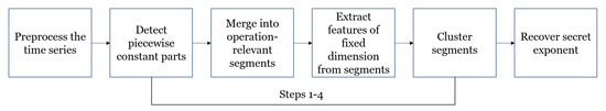
Figure 1. Whole process for our approach.

We defined each step, rather than one whole global model that segments time series and searches cluster (i.e., some function $h(·),c^{*}=h\left({\mathbf{y}}_{1:T}\right)$) due to the high complexity of that model, if it exists.

2.2.1. Change Point Detection

We have found from the power trace that there is an idle period or a piece-wise constant between operations of binary exponentiation, square and multiplication. Exploring this period is the most important part of whole work since segments divided only by the exact locations of operations will have similar patterns. We can model solving change point detection problem (with their number unknown) [17]. However we do not adopt reversible jump MCMC [18,19]. In this subproblem embedding the change point detection algorithm, we only find idle periods and incomplete segments are made. We then make complete(operation-relevant) segments by combining the incomplete segments in Section 2.2.2. Reason behind dividing two steps is that first, we do not have any information about the key or the shape of power trace of each operation and change point detecting problem whose number of change points are not known is already complex enough to avoid putting detection of constants and unknown shapes together into model. For detecting piece-wise constants, we can define by Bayes’ theorem the posterior distribution of change points $r_{1:T}$, $p\left(r_{1:T}\right|{\mathbf{y}}_{1:T},\theta )$ and our goal as:

$$\begin{array}{ll}p\left(r_{1:T}\right|{\mathbf{y}}_{1:T},\theta )& =\frac{p(r_{1:T},{\mathbf{y}}_{1:T},\theta )}{p\left({\mathbf{y}}_{1:T}\right|\theta )}\hfill \\ & \propto p(r_{1:T},{\mathbf{y}}_{1:T},\theta )\hfill \\ & =p\left({\mathbf{y}}_{1:T}\right|r_{1:T},\theta )p\left(r_{1:T}\right|\theta ),\hfill \end{array}$$

(2)

$${\overline{r}}_{1:T}={\mathbb{E}}_{p\left(r_{1:T}\right|{\mathbf{y}}_{1:T},\theta )}\left[r_{1:T}\right].$$

(3)

2.2.2. Merging Segments

As mentioned above, in this subproblem, we merge incomplete segments to complete segments whose start and end points indicate the start and end points of the operation. The goal here is building the merging function $g(·)$ as

$$r_{1:T}^M=g({\overline{r}}_{1:T},{\mathbf{y}}_{1:T}).$$

(4)

Only merging but not splitting is allowed in function $g(·)$, so $K_{r^M}\le K_r$ and $\left\{{\tau }_k^M\right|1\le k\le K_{r^M}\}\in \left\{{\overline{\tau }}_k\right|1\le k\le K_{\overline{r}}\}$ holds.

2.2.3. Extracting Features from Time Series Segments

It is known that previous correlation power analysis attacks have used power traces or parts of power traces that are cut in the same length. However, the lengths of power traces (or their parts) are not guaranteed to have the same length. Therefore, the model or algorithm for extracting information relevant to each operation must be capable of treating subsignals in different length. In this part, given the segments in different lengths, we extract the features that will be the input to the clustering part which needs fixed dimension.

$$\mathsf{\Phi }={[{\overline{\varphi }}_1,\cdots ,{\overline{\varphi }}_k,\cdots ,{\overline{\varphi }}_K]}^T,$$

(5)

where each row ${\overline{\varphi }}_k={[{\varphi }_{(k,1)},\cdots ,{\varphi }_{(k,d)}]}^T$ is a feature vector of k-th segment. The goal of this subproblem is building the feature extractor $f(·)$ that is capable of coping with the segments in different lengths

$${\overline{\varphi }}_k=f({\mathbf{y}}_{{\tau }_k:{\tau }_{k+1}-1},r_{1:T}^M).$$

(6)

2.2.4. Clustering Features

The last step is clustering all the segments with features extracted. Clustering is an unsupervised machine learning approach that assigns each data point a cluster based on similarity (or distance). After all the segments are assigned the clusters, we can find the key exponent. Our goal is identifying three clusters of features. In general, if the number of clusters is not known, optimizing the number of clusters is required. From this point of view, the number of clusters should be carefully considered to obtain highly accurate performance, but we can easily put three on it since there are only three patterns we look for, which are square, multiplication and the idle period between operations. After we identify the clusters, it becomes a trivial problem to decide which operation or period is related to one of clusters.

$$c_k^{*}=arg\underset{c\in \{Idle,Square,Multiply\}}{min}\left|\right|{\overline{\varphi }}_k-\frac{{\displaystyle \sum _{k=1:K_{r^M}}}{\overline{\varphi }}_k\mathbb{I}(c_k=c)}{{\displaystyle \sum _{k=1:K_{r^M}}}\mathbb{I}(c_k=c)}{\left|\right|}_2^2.$$

(7)

3. Proposed Approach

3.1. Preprocessing

There are many countermeasures to side channel analysis including the random noise addition. In order to deal with the random noise addition, we sample each power trace with the median filter. The median filter will decrease the effect of noise and reflect the trend of power signal. We apply the median filter to the power trace. We use the stride size equal to the window length. As a result, we reduce the length of power trace to analyze. Since the magnitude of power trace is a positive value, we use the absolute value of the power trace:

$${{}_{\mathbf{y}}}_{1:T}=\mathrm{MEDSAMPLE}\left(\right|P_{1:N_P}|,N_w),$$

(8)

where $N_P$ is a length of the original power trace and $N_w$ is window size. Figure 2 shows the effect of preprocessing the power traces.

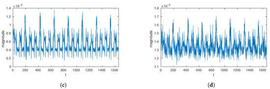
Figure 2. Raw and noise-added power traces preprocessing with median sampling. (a) Power trace; (b) Noise-added trace; (c) Median-sampled power trace; (d) Noise-added and median-sampled power trace.

3.2. Change Point Detection

3.2.1. Posterior Distribution

As mentioned above, the model here detects the piecewise constant part from the time series.

$$\begin{array}{c}\hfill y_t=m_k+ϵ,\end{array}$$

(9)

where random variable $m_k\sim \mathcal{N}(\mu ,V)$ is a mean of time series between ${\tau }_k$ and ${\tau }_{k+1}-1$ and $ϵ\sim \mathcal{N}(0,{\sigma }^2)$. The likelihood that ${\mathbf{y}}_{1:T}$ is observed given $r_{1:T}$, $m_{1:K_r}$ and $\theta$ is

$$\begin{array}{ll}p\left({\mathbf{y}}_{1:T}\right|r_{1:T},m_{1:K_r},\theta )& ={\displaystyle \prod _{k=1}^{K_r}}{\displaystyle \prod _{t={\tau }_k}^{{\tau }_{k+1}-1}}\mathcal{N}(y_t;m_k,{\sigma }^2)\hfill \\ & ={\left(\frac{1}{2\pi {\sigma }^2}\right)}^{-\frac{n}{2}}exp\left(-\frac{1}{2{\sigma }^2}{\displaystyle \sum _{k=1}^{K_r}}{\displaystyle \sum _{t={\tau }_k}^{{\tau }_{k+1}-1}}{(y_t-m_k)}^2\right).\hfill \end{array}$$

(10)

By conjugacy of the exponential family [20], posterior distribution of $m_{1:K_r}$ is also Gaussian. $m_k\sim \mathcal{N}(\frac{V{\overline{\mathbf{y}}}_k+{\sigma }^2\mu }{V+{\sigma }^2},\frac{V{\sigma }^2}{n_k(V+{\sigma }^2)})$, where ${\overline{\mathbf{y}}}_k=\frac{{\sum }_{t={\tau }_k}^{{\tau }_{k+1}-1}{y}_t}{{\tau }_{k+1}-{\tau }_k}$ and $n_k={\tau }_{k+1}-{\tau }_k$. If we plug the probability of $m_{1:K_r}$ into Equation (10), we get by identification,

$$\begin{array}{ll}p& \left(m_{1:K_r}\right|{\mathbf{y}}_{1:T},r_{1:T},\theta )\times p\left({\mathbf{y}}_{1:T}\right|r_{1:T},\theta )\\ & =p({\mathbf{y}}_{1:T},m_{1:K_r}|r_{1:T},\theta )\hfill \\ & =\left[\prod _{k=1}^{K_r}\prod _{t={\tau }_k}^{{\tau }_{k+1}-1}\mathcal{N}({\mathbf{y}}_t;m_k,{\sigma }^2)\right]\times \prod _{k=1}^{K_r}\mathcal{N}(m_k;\mu ,V)\hfill \\ \hfill & =\prod _{k=1}^{K_r}\mathcal{N}\left(m_k;\frac{V{\overline{\mathbf{y}}}_k+{\sigma }^2\mu }{V+{\sigma }^2},\frac{V{\sigma }^2}{n_k(V+{\sigma }^2)}\right)\hfill \\ \hfill & \times {\left(\frac{1}{2\pi {\sigma }^2}\right)}^{-\frac{n}{2}}{\left(\frac{V+{\sigma }^2}{{\sigma }^2}\right)}^{\frac{-K_r}{2}}exp\left(-\frac{1}{2(V+{\sigma }^2)}\sum _{k=1}^{K_r}{(y_t-\mu )}^2+\frac{V}{{\sigma }^2}\sum _{k=1}^{K_r}\sum _{t={\tau }_k}^{{\tau }_{k+1}-1}{(y_t-{\overline{\mathbf{y}}}_k)}^2\right).\hfill \end{array}$$

(11)

Therefore, we can get from Equation (11),

$$p\left({\mathbf{y}}_{1:T}\right|r_{1:T},\theta )={\left(\frac{1}{2\pi {\sigma }^2}\right)}^{-\frac{n}{2}}{\left(\frac{V+{\sigma }^2}{{\sigma }^2}\right)}^{\frac{-K_r}{2}}exp\left(-\frac{1}{2(V+{\sigma }^2)}\sum _{k=1}^{K_r}{(y_t-\mu )}^2+\frac{V}{{\sigma }^2}\sum _{k=1}^{K_r}\sum _{t={\tau }_k}^{{\tau }_{k+1}-1}{(y_t-{\overline{\mathbf{y}}}_k)}^2\right).$$

(12)

The trivial solution for this problem is to make every point as a change point, so that the sum of errors becomes least. In order to avoid this situation we have to model the number of change points $K_r$. We modelled the prior distribution to control the number of change points as Bernoulli distribution.

$$\begin{array}{cc}\hfill p\left(r_{1:T}\right|\lambda )& ={\lambda }^{K_r}{(1-\lambda )}^{n-K_r}.\hfill \end{array}$$

(13)

By Bayes’ theorem we can model the posterior distribution of random variable $r_{1:T}$ by putting Equation (11) and (13) together as follows:

$$\begin{array}{ll}p\left(r_{1:T}\right|{\mathbf{y}}_{1:T},\theta )& =\frac{p(r_{1:T},{\mathbf{y}}_{1:T}|\theta )}{p\left({\mathbf{y}}_{1:T}\right|\theta )}\hfill \\ \hfill & \propto p(r_{1:T},{\mathbf{y}}_{1:T}|\theta )\hfill \\ \hfill & =p\left({\mathbf{y}}_{1:T}\right|r_{1:T},\sigma )p\left(r_{1:T}\right|\lambda ).\hfill \end{array}$$

(14)

Joint distribution of $r_{1:T}\mathrm{and}{\mathbf{y}}_{1:T}$, $p(r_{1:T},{\mathbf{y}}_{1:T}|\theta )$ is needed since the evidence of the observation $p\left({\mathbf{y}}_{1:T}\right|\theta )$ is intractable to compute.

$$\begin{array}{ll}p& (r_{1:T},{\mathbf{y}}_{1:T}|\theta )\hfill \\ & =p\left({\mathbf{y}}_{1:T}\right|r_{1:T},\sigma )p\left(r_{1:T}\right|\lambda )\hfill \\ & ={\left(\frac{1}{2\pi {\sigma }^2}\right)}^{-\frac{n}{2}}{\left(\frac{V+{\sigma }^2}{{\sigma }^2}\right)}^{\frac{-K_r}{2}}exp\left(-\frac{1}{2(V+{\sigma }^2)}{\displaystyle \sum _{k=1}^{K_r}}{(y_t-\mu )}^2+\frac{V}{{\sigma }^2}{E}_{r_{1:T}}\right)\times {\lambda }^{{\sum }_{t=1}^T{r}_t}{(1-\lambda )}^{n-{\sum }_{t=1}^T{r}_t}\hfill \\ & =Z({\mathbf{y}}_{1:T},\theta )exp(-H\left(r_{1:T}\right)),\hfill \end{array}$$

(15)

where energy function of $r_{1:T}$, $H\left(r_{1:T}\right)=\frac{V}{2{\sigma }^2({\sigma }^2+V)}{E}_{r_{1:T}}+\gamma K_r$, $E_{r_{1:T}}={\displaystyle \sum _{k=1}^{K_r}}{\displaystyle \sum _{t={\tau }_k}^{{\tau }_{k+1}-1}}{(y_t-m_k)}^2$, $\gamma =\frac{1}{2}log\left(\frac{{\sigma }^2+V}{{\sigma }^2}\right)+log\left(\frac{1-\lambda }{\lambda }\right)$ and $Z({\mathbf{y}}_{1:T},\theta )$ is an intractable normalizing constant.

3.2.2. Markov Chain Monte Carlo

We use Markov Chain Monte Carlo(MCMC) to find the global optimal solution [21,22] for the model we designed. In Reference [19], $m_k$ was also the random variable to infer and apply reversible jump MCMC to cope with changing dimension (the number of $m_k$s to estimate), but our work considers only $r_{1:T}$ and replace $m_k$ with ${\overline{\mathbf{y}}}_k$ and simulate only for change points.

We detect the piecewise constants by computing the expectation of random variable $r_{1:T}$,

$$\begin{array}{ll}{\overline{r}}_{1:T}& ={\mathbb{E}}_{p\left(r_{1:T}\right|{\mathbf{y}}_{1:T},\theta )}\left[r_{1:T}\right]=\int p\left(r_{1:T}\right|{\mathbf{y}}_{1:T},\theta )r_{1:T}\mathrm{d}{r}_{1:T},\hfill \\ \hfill {\widehat{r}}_{1:T}& =\frac{1}{n}{\displaystyle \sum _{s=1}^n}{r}_{1:T}^s,\hfill \\ \hfill {\widehat{r}}_{1:T}& \approx {\overline{r}}_{1:T},\hfill \end{array}$$

(16)

where ${\overline{r}}_{1:T}$ is a true mean of $r_{1:T}$ and ${\widehat{r}}_{1:T}$ is an Monte Carlo estimate of $r_{1:T}$ when $r_{1:T}^s\sim p\left(r_{1:T}\right).$ The last part holds when $n\to \infty .$

Instead of generating samples from the intractable posterior distribution $p\left(r_{1:T}\right|{\mathbf{y}}_{1:T},\theta )$, we propose a function from which is easy to draw samples, namely proposal function(Metropolis-Hastings, Algorithm 1). We can think of two proposal functions regarding the property of change point detection problem. Given one sample, one of change points can be popped and two segments are merged or one change point is born and segment is split. Either case, this is reverting $r_t$, $0\to 1$, or $1\to 0$. The other proposal function is a swap between $0\leftrightarrow 1$.

Algorithm 1 Metroplis Hastings

procedureMH($p(·),q(·),r_{1:T}^0,n$)         ▹ posterior, proposal and initial sample, number of samples      for $s=1,2,\cdots ,$ n do           $r_{1:T}^{*}\sim q\left(r_{1:T}^{*}\right|r_{1:T}^{s-1})$           $\alpha \leftarrow \frac{p\left(r_{1:T}^{*}\right)q\left(r_{1:T}^{s-1}\right|r_{1:T}^{*})}{p\left(r_{1:T}^{s-1}\right)q\left(r_{1:T}^{*}\right|r_{1:T}^{s-1})}$           $a\leftarrow min(1,\alpha )$           $u\sim \mathcal{U}(0,1)$           if $u<a$ then               $r_{1:T}^s\leftarrow r_{1:T}^{*}$           else               $r_{1:T}^s\leftarrow r_{1:T}^{s-1}$                return $r_{1:T}^1,r_{1:T}^2,\cdots ,r_{1:T}^n$

The proposal function for MCMC is succession of reverting and swapping with probability of

$$\begin{array}{c}\hfill q\left(r_{1:T}^{*}\right|r_{1:T})=\left\{\begin{array}{cc}\frac{1}{T},\hfill & \mathrm{if}\mathrm{revert}\hfill \\ \frac{1}{K_r(T-K_r)},\hfill & \mathrm{if}\mathrm{swap}.\hfill \end{array}\right.\end{array}$$

(17)

This proposal probability is reducible, when calculated in Metropolis-Hastings, to

$$\begin{array}{c}\hfill \alpha =\frac{p\left(r_{1:T}^{*}\right)q\left(r_{1:T}^{s-1}\right|r_{1:T}^{*})}{p\left(r_{1:T}^{s-1}\right)q\left(r_{1:T}^{*}\right|r_{1:T}^{s-1})}=\frac{p\left(r_{1:T}^{*}\right)}{p\left(r_{1:T}^{s-1}\right)},\end{array}$$

(18)

since in reverting case the probability only depends on the length of the sample and in swapping case the number of change points does not change ($K_{r^{s-1}}=K_{r^{*}}$).

Figure 3 shows the ${\overline{r}}_{1:T}$ obtained from MCMC section. However this model only detects the piecewise constants, so non-constant parts (i.e., drastic changes) are all high in probability of being change points.

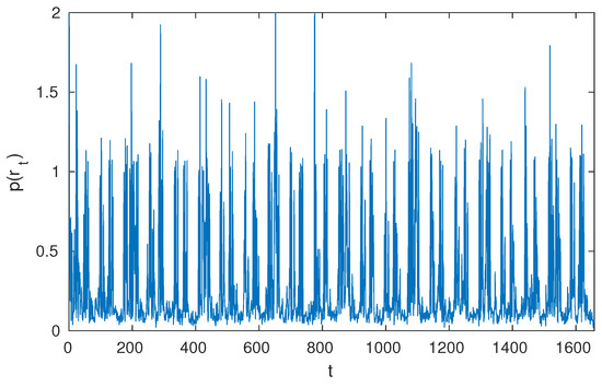
Figure 3. Approximate expectation of $r_t$.

3.3. Merging Segments

In Reference [23], it is shown that by controlling parameter and adopting various models, various goals can be achieved more than just detecting piecewise constants. However, we assume the least about the data that adopted merging segments part. The change points obtained from Section 3.2 indicate the locations where mean of each segment is changed. Therefore, when operations are executed, it is likely that the operation part is split into many segments and there are more than one change points. We detect whether segments are from the operation part or the idle part and merge segments from the operation part. We consider the following two properties of the idle part.

• Whether the length of segment is long enough to be a segment
• Whether the segments suspected as idle periods lie on similar level of power

Details for merging segments are on Algorithm 2 below. Figure 4 shows merged segments.

Algorithm 2 Merge Segments

procedureMerge(${\overline{r}}_{1:T},{\mathbf{y}}_{1:T}$)     Initialize vector $len\_seg[1:K_{\overline{r}}]$ with kth element as ${\tau }_{k+1}-{\tau }_k$     Initialize vector $mean[1:K_{\overline{r}}]$ with kth element as ${\overline{\mathbf{y}}}_k$     $[sorted\_mean[1:K_{\overline{r}}],Index[1:K_{\overline{r}}]]\leftarrow \mathrm{SORT}\left(mean\right)$        ▹ in descending order     $best\_so\_far\leftarrow -\infty$     $TH\leftarrow 0$     for $k=1,2,\cdots ,K_{\overline{r}}$ do         $mean\_iter\leftarrow (T-{\sum }_{i=1}^{k}len\_seg\left[Index\left[i\right]\right])\times k$         if $best\_so\_far<mean\_iter$ then            $best\_so\_far\leftarrow mean\_iter$            $TH\leftarrow k$              $Inde{x}^{*}\leftarrow \left\{Index\left[i\right]\right|TH\le i\le T\}$     for $t=1,2,\cdots ,T$ do         $r^M\left[t\right]\leftarrow \left\{\begin{array}{ll}1\hfill & \mathrm{if}t\in \left\{{\tau }_i\right|i\in Inde{x}^{*}\}\hfill \\ 0& \mathrm{otherwise}.\end{array}\right.$          return $r_{1:T}^M=r^M[1:T]$

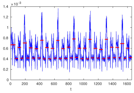
Figure 4. Change points and mean of each segment based on $r_{1:T}^M$.

3.4. Extracting Features from Time Series Segments

In this part, we extract features of fixed dimension from the segments. That is, given the segment ${\mathbf{y}}_{{\tau }_k:{\tau }_{k+1}-1}$, we compute feature of fixed dimension ${\overline{\varphi }}_k$. We applied two approaches to extract the features and this part is to be further researched.

3.4.1. Polynomial Least Square Coefficients

First approach we apply is polynomial fitting. Polynomial model has its form as below:

$$y_i={\beta }_0+{\beta }_1{x}_i+{\beta }_2{x}_i^2+\cdots +{\beta }_{D-1}{x}_i^{D-1}+ϵ={\mathbf{\beta }}^T{\mathbf{x}}_i+ϵ,$$

where ${\beta }_d$ is a dth parameter which describes the influence of $x^d$ on y and $\mathbf{\beta }={[{\beta }_0,{\beta }_1,{\beta }_2,\cdots ,{\beta }_{D-1}]}^T,{\mathbf{x}}_i={[1,x_i,x_i^2,\cdots ,x_i^{D-1}]}^T$. The solution to polynomial fitting with minimum least squared error exists in closed form:

$$\widehat{\mathbf{\beta }}={\left(X^{T}X\right)}^{-1}{X}^T\mathbf{y},$$

where n-by-D matrix $X={[{\mathbf{x}}_1,{\mathbf{x}}_2,\cdots ,{\mathbf{x}}_n]}^T$ is concatenation of n data samples. Now that each segment is given, for segment ${\mathbf{y}}_{{\tau }_k:{\tau }_{k+1}-1}$, let $X_k={[{\mathbf{x}}_{{\tau }_k},{\mathbf{x}}_{{\tau }_k+1},\cdots ,{\mathbf{x}}_{{\tau }_{k+1}-1}]}^T$ and ${\mathbf{x}}_t={[1,t,t^2,\cdots ,t^{D-1}]}^T,{\tau }_k\le t\le {\tau }_{k+1}-1$. Then we can estimate ${\widehat{\mathbf{\beta }}}_k$ for each segment of time series and let it be a D-by-1 feature of each segment as follows:

$${\overline{\varphi }}_k={\widehat{\mathbf{\beta }}}_k={\left(X_k^T{X}_k\right)}^{-1}{X}_k^T{\mathbf{y}}_{{\tau }_k:{\tau }_{k+1}-1}.$$

We visualize coefficients by reconstructing power traces in Figure 5.

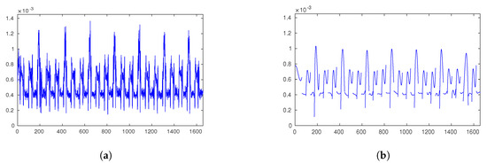
Figure 5. Time series and reconstruction with polynomial coefficients. (a) Time series; (b) Polynomially reconstructed time series.

3.4.2. Histogram

The second approach is making a histogram out of each segment. Each histogram shares the same scale level of bins. The size of one bin is $\frac{max{y}_{1:T}-min{y}_{1:T}}{D}$. Once we normalize the histogram to sum up to 1, this gives a distribution of each segment.

$${\overline{\varphi }}_k=Histogram(y_{{\tau }_k:{\tau }_{k+1}-1},D)$$

3.5. Clustering Features

In this part, we finally make clusters of the features so that we can match each segment to the operation which has been executed when generating the segment. We apply K-means clustering algorithm. Based on the pre-defined distance measure and number of clusters, the K-means algorithm repeats until convergence assigning data points to cluster based on distance and computing the mean of each cluster [20]. We assigned number of clusters K = 3 based on the number of operations (Square, Multiply and optionally idle period). For coefficients of Section 3.4.1, Euclidean distance $Distance({\overline{\varphi }}_i,{\overline{\varphi }}_j)=\sqrt{{\left[({\overline{\varphi }}_i-{\overline{\varphi }}_j)\right]}^T\left[({\overline{\varphi }}_i-{\overline{\varphi }}_j)\right]}$ is defined. For histogram coefficients of Section 3.4.2, both Euclidean distance and symmertrized divergence $Distance({\overline{\varphi }}_i,{\overline{\varphi }}_j)=KL\left({\overline{\varphi }}_i\right|{\overline{\varphi }}_j)+KL\left({\overline{\varphi }}_j\right|{\overline{\varphi }}_i)$ (only for normalized histogram) are defined as distance measures. The performance of K-means algorithm, however, is affected by the initial points. So we run K-means algorithm multiple times and evaluate each run [24]. Only with data we used should we evaluate each run so that any other information is not reflected and result of K-means is evaluated fairly. We adopt Davies-Bouldin index(DB index) to evaluate each run and choose best performing clusters. Desirable clusters, with high inter-cluster distance and low intra-cluster distance, produce low DB index [25]. Figure 6 shows recovering key exponent.

Figure 6. Key exponent recovery process. (a) t-SNE visualized polynomial coefficients clustered; (b) Recovering key exponent with the clusters.

4. Experiments and Results

The experiments were conducted under the environment below:

• The window size $N_w$ is 1000, $N_p$ is dependent on input data, which in our experiment is 1,657,401.
• Hyperparameters were selected as follows: $\lambda =48/T,\sigma =9.644e-05,V=7.377-e07,$$\mu =\frac{{\sum }_{t=1}^T{y}_t}{T}$
• Binary exponentiation of RSA 16-bit algorithm was executed on Samsung Galaxy S3 smartphone. Electromagnetic wave was sampled by oscilloscope. Sampling rate was 500 MS/s.

As mentioned, $\lambda$ controls the number of change points. The best guess about the key exponents without any knowledge is a half of 1s and the other half of 0s. The number of change points will then be 48 (= 2×(16 + 8)) as bit of 0 leads to only square operation and bit of 1 leads to square and multiplication. The best guess for $\mu$ is the mean of the time series. Though $\sigma$ and V should be optimized for the best inference, we have experimentally chosen the values of $\sigma$ and V among the candidates that were sampled during MCMC process.

Our approach is evaluated with criteria below:

• To which level of noise added and inserted to signal (Signal to Noise Ratio, SNR) does the approach work
• The quality of clusters with external information

The first criterion shows the robustness of the approach to the noise whereas adding noise is often suggested as a countermeasure to the side channel analysis. For the second criterion, the external information (information not used for making clusters) we adopt is the very key exponent we want to estimate.

4.1. Comparison with Naive Peak Detection

This experiment focuses on comparing the proposed approach to naive correlation peak detecting method. Figure 7a was obtained by computing covariance with the entire signal and sliding window size of 100. The most general sliding window is starting with the first part and sliding window size was selected as 100 in a ’naive’ way. As seen in Figure 7b, peaks were found to satisfy two thresholds: covariance is positive and minimum distance between two nearest peaks is larger than 20 in time scale. Without these thresholds, too many irrelevant peaks were found. Our approach showed better performance in finding the locations of the executed operations and finding that of inserted noise.

Figure 7. Cross-covariance and peaks. (a) Cross-covariance with sliding window; (b) Peaks on cross-covariance.

Stems are drawn on $r_{1:T}^M$ and peaks in Figure 8a,b. Noise inserted are located on time series from $t=759$ to $t=924$. The proposed method successfully finds out the location of noise as well as other operations whereas naive method does not successfully find out the location of operations nor the inserted noise.

Figure 8. Comparison of two methods. (a) Proposed method; (b) Naive peak detection method.

4.2. Noise Level

We have experimented on 16 levels of noise. We incremented the ratio of the standard deviation of noise and the raw signal linearly by 0.2 up to 3.0. Table 1 shows how consistent our work is when a different level of noise is added. From the table, we see that when the ratio of standard deviation is 1.8, $K_{r_{1:T}}$ has changed. From that, the number of change point keeps changing although with some level of noise it remained 44. When the noise is added, the change point changes and sometimes its number also changes.

Table 1. The number of change points with respect to noise level (True $K=44$).

std(noise)/std(signal)	0	0.2	0.4	0.6	0.8	1.0	1.2	1.4
SNR(db)	-	13.98	7.96	4.44	1.94	0.0	−1.58	−2.91
$K_{r_{1:T}}$	44	44	44	44	44	44	44	44
std(noise)/std(signal)	1.6	1.8	2.0	2.2	2.4	2.6	2.8	3.0
SNR(db)	−4.07	−5.09	−6.01	−6.84	−7.60	−8.29	−8.94	−9.53
$K_{r_{1:T}}$	44	45	47	44	47	44	48	58

For comparing ${\tau }_{1:K}$, we have chosen only a standard deviation ratio of 0.2–1.6 since besides those, the numbers of change points have already been changed. Average absolute error on ${\tau }_{1:K}$ compared to signal without noise is computed as $\frac{{\sum }_{k=1}^{K_{r_{1:T}}}|{\tau }_k^{raw}-{\tau }_k^{noised}|}{K_{r_{1:T}}}$. Table 2 shows that average absolute error is no more than 3, and especially for noise level 0.2, 0.4 and 0.6, the average absolute error is less than 1.

Table 2. Error on ${\tau }_{1:K}$ with respect to noise level.

std(noise)/std(signal)	0.2	0.4	0.6	0.8	1.0	1.2	1.4	1.6
SNR(db)	13.98	7.96	4.44	1.94	0.0	−1.58	−2.91	-4.07
$\frac{{\sum }_{k=1}^{K_{r_{1:T}}}|{\tau }_k^{raw}-{\tau }_k^{noised}|}{K_{r_{1:T}}}$	0.5	0.5	0.89	1.25	1.23	1.77	2.34	2.39

4.3. External Information

Next we compared clusters with external information, the actual key exponent. This is not a part of our approach since the actual key exponent is used. This part rather evaluates our approach to compare our estimate with the label. Table 3 shows the the average accuracy of 100 runs of the K-means algorithm. We used polynomial coefficients to 3rd degree ($D=4$) and for the histogram we used $D=60$. Clustering polynomial least square coefficient features are not affected much by the noise level whereas clustering histogram features are relatively more affected by noise. We made a confusion matrix of actual key exponents and clusters assigned to segments. Accuracy of the cluster is defined as $Accuracy\left(Cluster\right)=\frac{{\displaystyle \sum _{i=j}}{C}_{i,j}}{{\displaystyle \sum _{i,j}}{C}_{i,j}},$ where $C_{i,j}$ is element of the confusion matrix.

	Cluster Idle	Cluster Square	Cluster Multiply
Idle	$C_{1,1}$	$C_{1,2}$	$C_{1,3}$
Square	$C_{2,1}$	$C_{2,2}$	$C_{2,3}$
Multiply	$C_{3,1}$	$C_{3,2}$	$C_{3,3}$

Table 3. Mean Accuracy of 100 runs.

std(noise)/std(signal)	0	0.2	0.4	0.6	0.8	1.0	1.2	1.4	1.6
SNR(db)	-	13.98	7.96	4.44	1.94	0.0	−1.58	−2.91	−4.07
Polynomial coeffs	95.82	95.64	95.57	98.11	99.20	95.75	99.45	98.05	97.36
Histogram	82.04	81.95	83.38	80.38	83.20	80.30	79.11	76.66	78.02

4.4. Recovering Key Exponent

Our approach should be feasible without the external information. That is, we should be able to distinguish more accurate runs of clustering from the others. Figure 9 shows the examples of desirable and undesirable runs of clustering. We sorted 100 DB indices in ascending order and picked 5, 10, and 15 lowest DB indices and corresponding clusters. Table 4 shows the the average accuracy of 5, 10 and 15 runs of the K-means algorithm. We can see huge improvement in most of the cases, especially in the histogram features. This means that even without the external information, we can distinguish the good and bad clusters and find the key exponents.

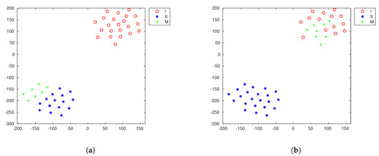
Figure 9. t-SNE visualized histogram features clustered. (a) Example of desirable cluster; (b) Example of undesirable cluster.

Table 4. Selecting desirable clusters with DB index.

std(noise)/std(signal)	0	0.2	0.4	0.6	0.8	1.0	1.2	1.4	1.6
SNR(db)	-	13.98	7.96	4.44	1.94	0.0	−1.58	−2.91	−4.07
Polynomial coeffs - 5	93.18	100.00	100.00	98.18	97.73	95.45	97.73	91.36	96.36
Polynomial coeffs - 10	94.77	100.00	100.00	99.09	98.86	97.73	97.73	90.91	93.18
Polynomial coeffs - 15	96.52	100.00	100.00	99.39	99.24	98.48	97.73	93.03	91.97
Histogram - 5	89.55	94.09	97.73	97.73	97.73	92.73	97.73	88.64	97.73
Histogram - 10	93.64	95.91	97.73	97.73	97.73	95.23	98.86	93.18	97.73
Histogram - 15	95.00	96.52	97.73	98.33	97.88	96.06	99.24	95.45	97.73

4.5. Data Scale

In this part, we empirically checked the time complexity of our approach. We have set the time series length $T=N_p/N_w$ differently in each case. Then we checked each case 10 times and box plotted in Figure 10. It shows that time spent in each case is linear to the time series length T. So if the raw data are in a larger sampling rate or a larger key bit size, our approach takes longer to that ratio.

Figure 10. Time spent by data scale.

5. Discussion

• For a longer key bit: If we can assume that the environment that generated the power trace is consistent during the whole time so that there exist certain patterns, we can apply our methods to the first part and extract some patterns from that part. For the rest, using the patterns we can find the key exponents faster. In this manner, we can solve the rest part of the problem in a supervised way, whereas our approach is a totally unsupervised way for finding a key. This will reduce the time spent on analysis even when the key length is relatively long.
• Weakness: One major weakness is that our approach is based on finding piece-wise constant parts. If the idle part changes drastically with a magnitude bigger than $\sigma$ or the idle part has another specific shape, we shall adopt a different model.
• Further application: the proposed approach of ours can be applied to other related applications. A discrete power system is one of the examples [26,27]. Problems of systems with different power generation models and different assumptions can be solved with the proposed approach.

6. Conclusions

In this work, we suggested a probabilistic model-based side channel analysis. We modelled a change point detection problem to detect piecewise constants which are not directly related to finding keys, and merged incomplete segments to key-relevant complete segments. We solved this problem with an MCMC approach to find a global optimal solution. From each segment, we extracted features of a fixed dimension and assigned a cluster to each segment. We showed that this cluster is highly related to key exponent of power trace and this approach consistently works even in the presence of the noise. We evaluated our approach with criteria of noise-level-robustness and accuracy of the key. The source code for our work is available at github.com/JeonghwanH/binEXP_CPD.

References

- Messerges, T.S.; Dabbish, E.A.; Sloan, R.H. Power analysis attacks of modular exponentiation in smartcards. In Proceedings of the International Workshop on Cryptographic Hardware and Embedded Systems, Worcester, MA, USA, 12–13 August 1999; Springer: Berlin/Heidelberg, Germany, 1999; pp. 144–157. [Google Scholar]
- Witteman, M.F.; van Woudenberg, J.G.; Menarini, F. Defeating RSA multiply-always and message blinding countermeasures. In Proceedings of the Cryptographers’ Track at the RSA Conference, San Francisco, CA, USA, 14–18 February 2011; Springer: Berlin/Heidelberg, Germany, 2011; pp. 77–88. [Google Scholar]
- Picek, S.; Heuser, A.; Jovic, A.; Ludwig, S.A.; Guilley, S.; Jakobovic, D.; Mentens, N. Side-channel analysis and machine learning: A practical perspective. In Proceedings of the 2017 International Joint Conference on Neural Networks (IJCNN), Anchorage, AK, USA, 14–19 May 2017; pp. 4095–4102. [Google Scholar]
- Lerman, L.; Bontempi, G.; Markowitch, O. Power analysis attack: An approach based on machine learning. IJACT 2014, 3, 97–115. [Google Scholar] [CrossRef]
- Benadjila, R.; Prouff, E.; Strullu, R.; Cagli, E.; Dumas, C. Study of deep learning techniques for side-channel analysis and introduction to ASCAD database. In ANSSI, France & CEA, LETI, MINATEC Campus, France; 2018; Volume 22, Available online: https://eprint.iacr.org/2018/053.pdf (accessed on 20 February 2020).
- Hettwer, B.; Gehrer, S.; Güneysu, T. Applications of machine learning techniques in side-channel attacks: A survey. J. Cryptogr. Eng. 2019, 1–28. [Google Scholar] [CrossRef]
- Clavier, C.; Feix, B.; Gagnerot, G.; Roussellet, M.; Verneuil, V. Horizontal correlation analysis on exponentiation. In Proceedings of the International Conference on Information and Communications Security, Barcelona, Spain, 15–17 December 2010; Springer: Berlin/Heidelberg, Germany, 2010; pp. 46–61. [Google Scholar]
- Bauer, A.; Jaulmes, E.; Prouff, E.; Wild, J. Horizontal and vertical side-channel attacks against secure RSA implementations. In Proceedings of the Cryptographers’ Track at the RSA Conference, San Francisco, CA, USA, 25 February–1 March 2013; Springer: Berlin/Heidelberg, Germany, 2013; pp. 1–17. [Google Scholar]
- Bauer, A.; Jaulmes, É. Correlation analysis against protected SFM implementations of RSA. In Proceedings of the International Conference on Cryptology in India, Mumbai, India, 7–10 December 2013; Springer: Berlin/Heidelberg, Germany, 2013; pp. 98–115. [Google Scholar]
- Clavier, C.; Feix, B.; Gagnerot, G.; Giraud, C.; Roussellet, M.; Verneuil, V. ROSETTA for single trace analysis. In Proceedings of the International Conference on Cryptology in India, Kolkata, India, 9–12 December 2012; Springer: Berlin/Heidelberg, Germany, 2012; pp. 140–155. [Google Scholar]
- Walter, C.D. Sliding windows succumbs to Big Mac attack. In Proceedings of the International Workshop on Cryptographic Hardware and Embedded Systems, Paris, France, 14–16 May 2001; Springer: Berlin/Heidelberg, Germany, 2001; pp. 286–299. [Google Scholar]
- Specht, R.; Heyszl, J.; Kleinsteuber, M.; Sigl, G. Improving non-profiled attacks on exponentiations based on clustering and extracting leakage from multi-channel high-resolution EM measurements. In Proceedings of the International Workshop on Constructive Side-Channel Analysis and Secure Design, Berlin, Germany, 13–14 April 2015; Springer: Berlin/Heidelberg, Germany, 2015; pp. 3–19. [Google Scholar]
- Heyszl, J.; Ibing, A.; Mangard, S.; De Santis, F.; Sigl, G. Clustering algorithms for non-profiled single-execution attacks on exponentiations. In Proceedings of the International Conference on Smart Card Research and Advanced Applications, Berlin, Germany, 27–29 November 2013; Springer: Berlin/Heidelberg, Germany, 2013; pp. 79–93. [Google Scholar]
- Batina, L.; Gierlichs, B.; Lemke-Rust, K. Differential cluster analysis. In Proceedings of the International Workshop on Cryptographic Hardware and Embedded Systems, Lausanne, Switzerland, 6–9 September 2009; Springer: Berlin/Heidelberg, Germany, 2009; pp. 112–127. [Google Scholar]
- Nascimento, E.; Chmielewski, Ł. Applying horizontal clustering side-channel attacks on embedded ECC implementations. In Proceedings of the International Conference on Smart Card Research and Advanced Applications, Lugano, Switzerland, 13–15 November 2017; Springer: Berlin/Heidelberg, Germany, 2017; pp. 213–231. [Google Scholar]
- Perin, G.; Chmielewski, Ł. A semi-parametric approach for side-channel attacks on protected RSA implementations. In Proceedings of the International Conference on Smart Card Research and Advanced Applications, Bochum, Germany, 4–6 November 2015; Springer: Berlin/Heidelberg, Germany, 2015; pp. 34–53. [Google Scholar]
- Lavielle, M.; Moulines, E. Least-squares estimation of an unknown number of shifts in a time series. J. Time Ser. Anal. 2000, 21, 33–59. [Google Scholar] [CrossRef]
- Green, P.J. Reversible jump Markov chain Monte Carlo computation and Bayesian model determination. Biometrika 1995, 82, 711–732. [Google Scholar] [CrossRef]
- Lavielle, M.; Lebarbier, E. An application of MCMC methods for the multiple change-points problem. Signal Process. 2001, 81, 39–53. [Google Scholar] [CrossRef]
- Bishop, C.M. Pattern Recognition and Machine Learning; Springer Science+ Business Media: Berlin/Heidelberg, Germany, 2006. [Google Scholar]
- Metropolis, N.; Rosenbluth, A.W.; Rosenbluth, M.N.; Teller, A.H.; Teller, E. Equation of state calculations by fast computing machines. J. Chem. Phys. 1953, 21, 1087–1092. [Google Scholar] [CrossRef]
- Hastings, W.K. Monte Carlo Sampling Methods Using Markov Chains and Their Applications; Oxford University Press: Oxford, UK, 1970. [Google Scholar]
- Lavielle, M. Optimal segmentation of random processes. IEEE Trans. Signal Process. 1998, 46, 1365–1373. [Google Scholar] [CrossRef]
- Arthur, D.; Vassilvitskii, S. k-means++: The advantages of careful seeding. In Proceedings of the Eighteenth Annual ACM-SIAM Symposium on Discrete Algorithms, New Orleans, LA, USA, 7–9 January 2007; Society for Industrial and Applied Mathematics: Philadelphia, PA, USA, 2007; pp. 1027–1035. [Google Scholar]
- Davies, D.L.; Bouldin, D.W. A cluster separation measure. IEEE Trans. Pattern Anal. Mach. Intell. 1979, PAMI-1, 224–227. [Google Scholar] [CrossRef]
- Dassios, I.K.; Szajowski, K.J. A non-autonomous stochastic discrete time system with uniform disturbances. In Proceedings of the IFIP Conference on System Modeling and Optimization, Sophia Antipolis, France, 29 June–3 July 2015; Springer: Berlin/Heidelberg, Germany, 2015; pp. 220–229. [Google Scholar]
- Dassios, I.K.; Szajowski, K.J. Bayesian optimal control for a non-autonomous stochastic discrete time system. Appl. Math. Comput. 2016, 274, 556–564. [Google Scholar] [CrossRef]
© 2020 by the authors. Licensee MDPI, Basel, Switzerland. This article is an open access article distributed under the terms and conditions of the Creative Commons Attribution (CC BY) license (http://creativecommons.org/licenses/by/4.0/).