Automatic Detection of Pulmonary Nodules using Three-dimensional Chain Coding and Optimized Random Forest

 ,
,  ,
, 
Abstract
1. Introduction
Related Works
2. Materials and Methods
2.1. LIDC-IDRI Dataset
2.2. Methods
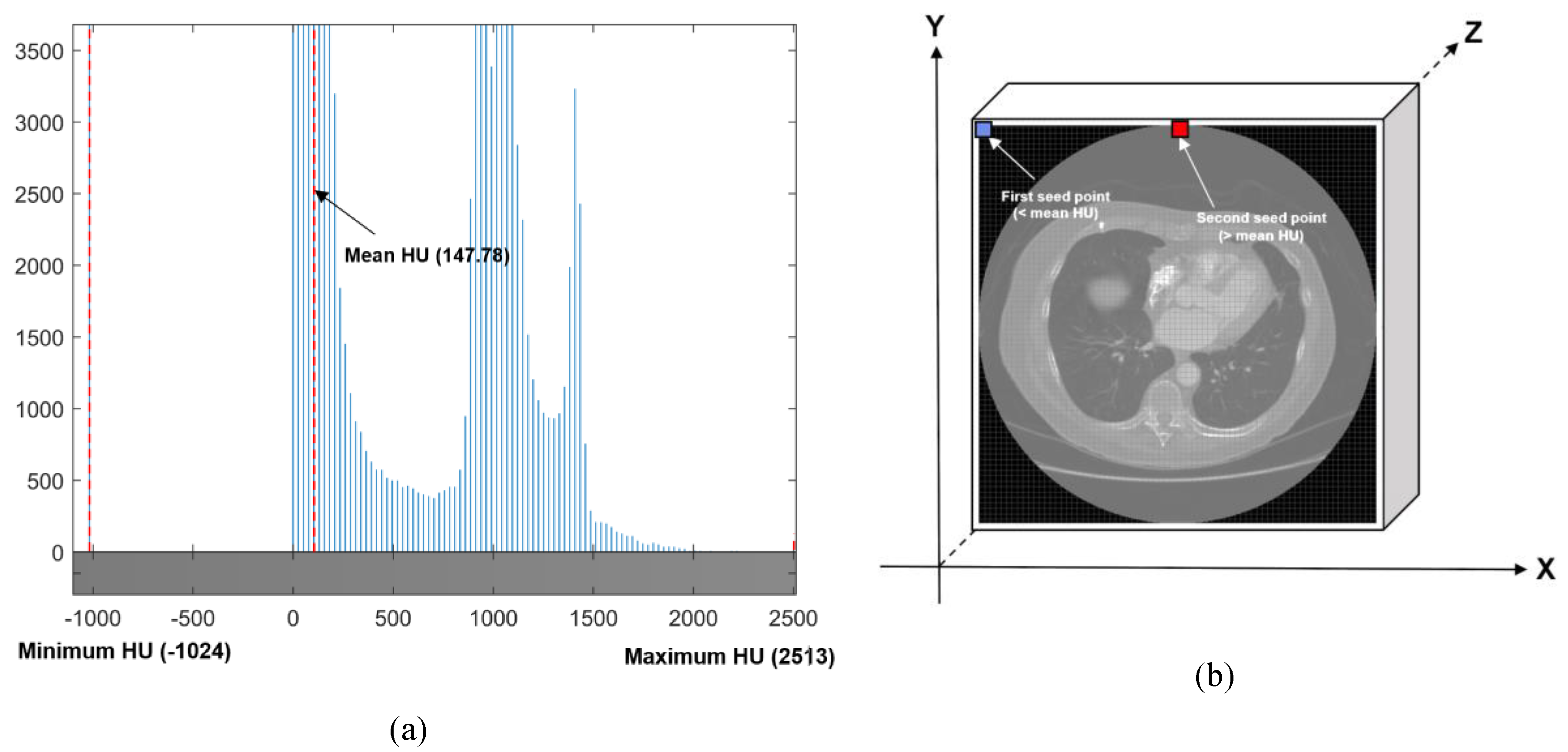
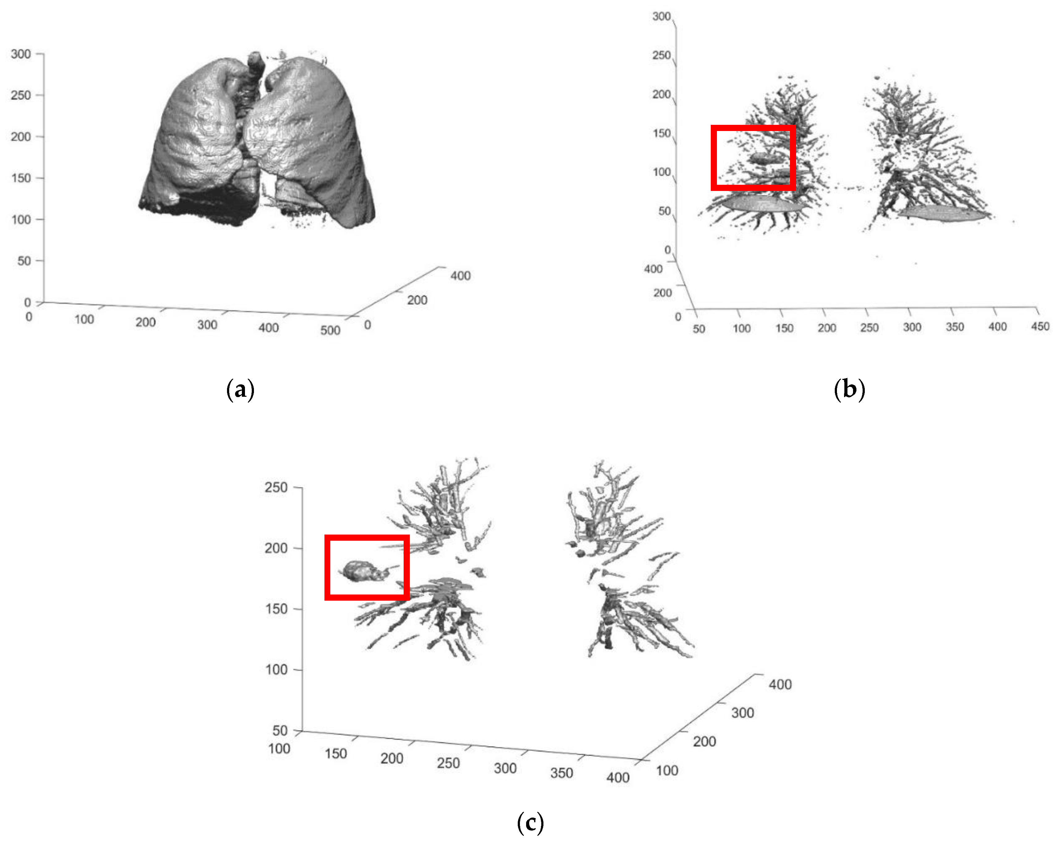
2.2.1. Automated Seeded Region Growing
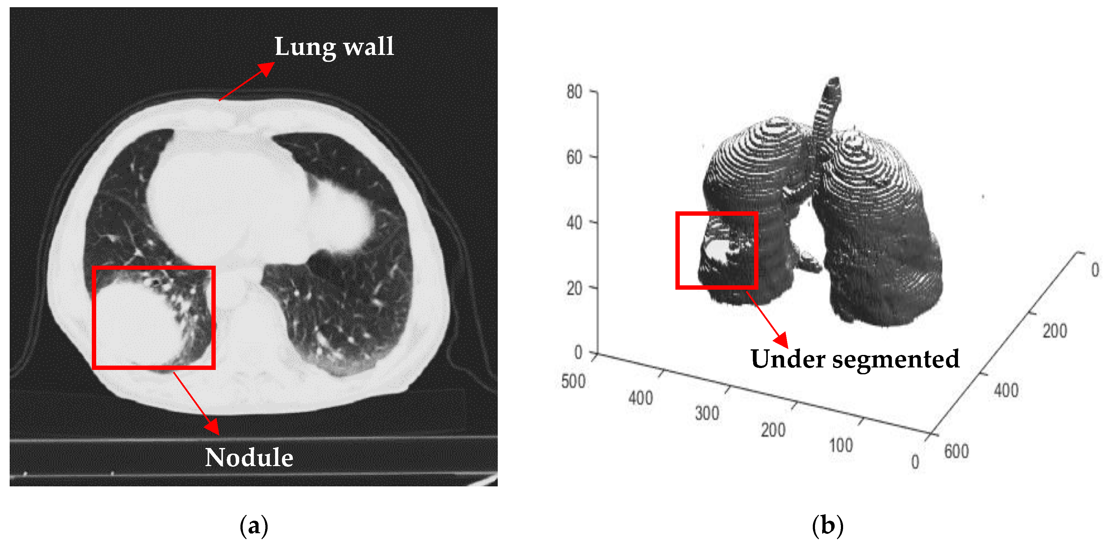
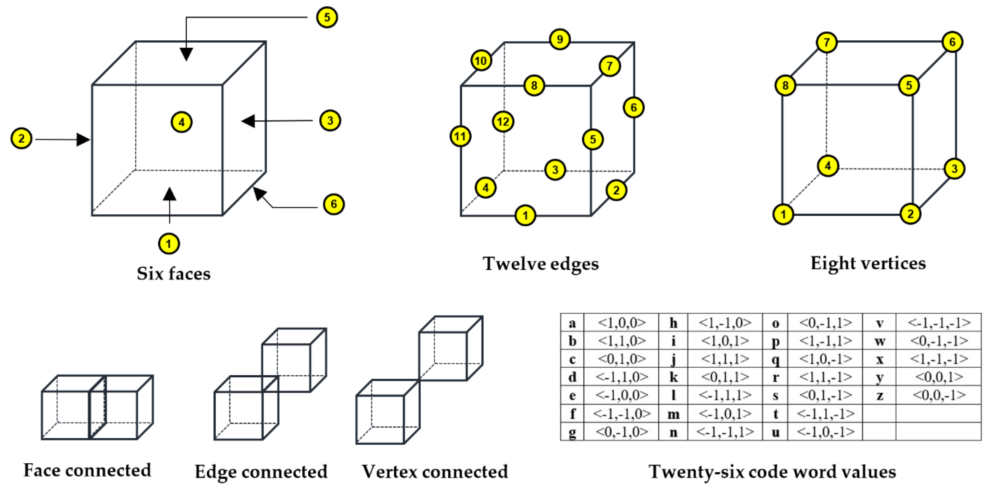
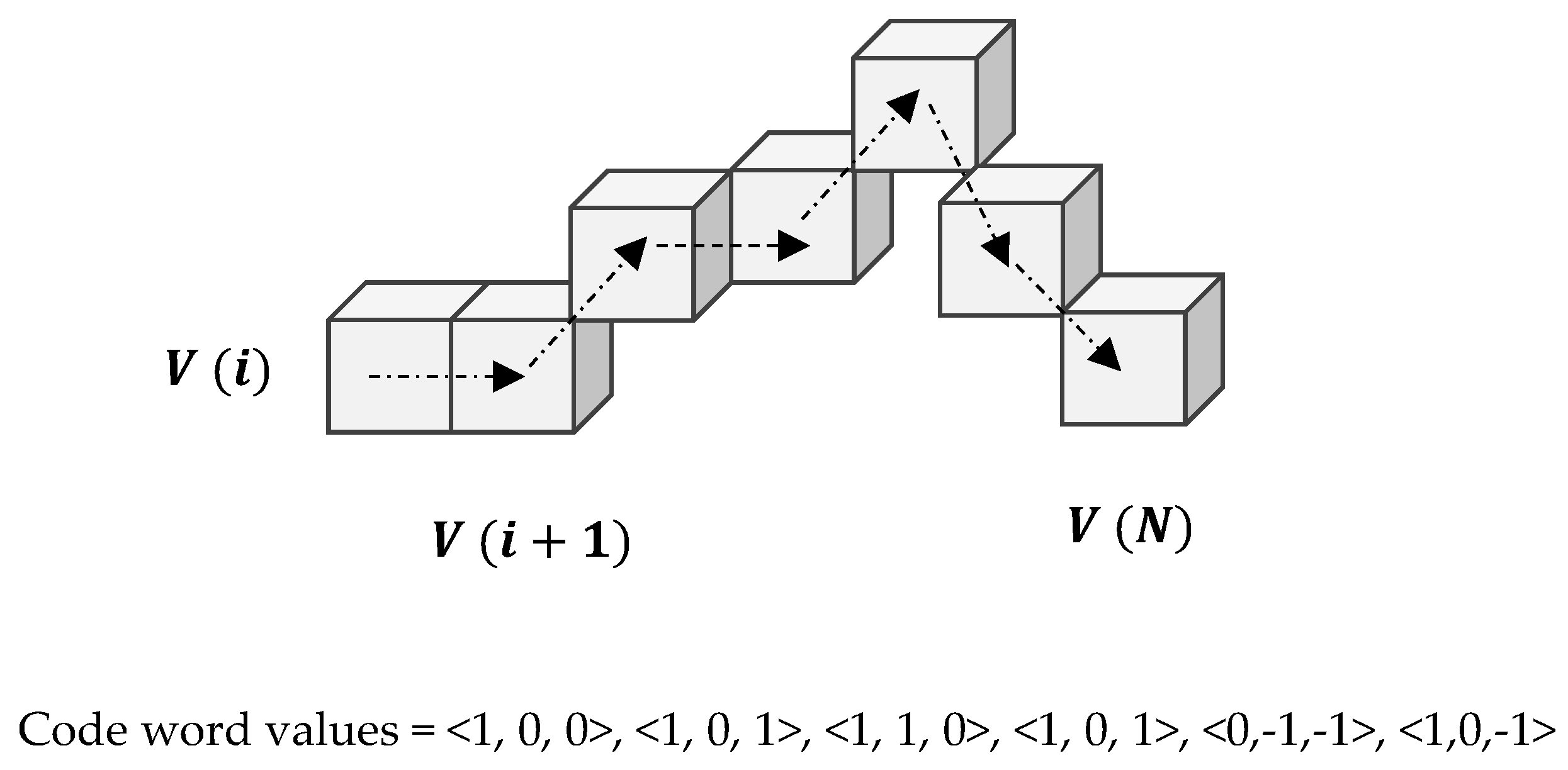
2.2.2. Three Dimensional Chain Coding
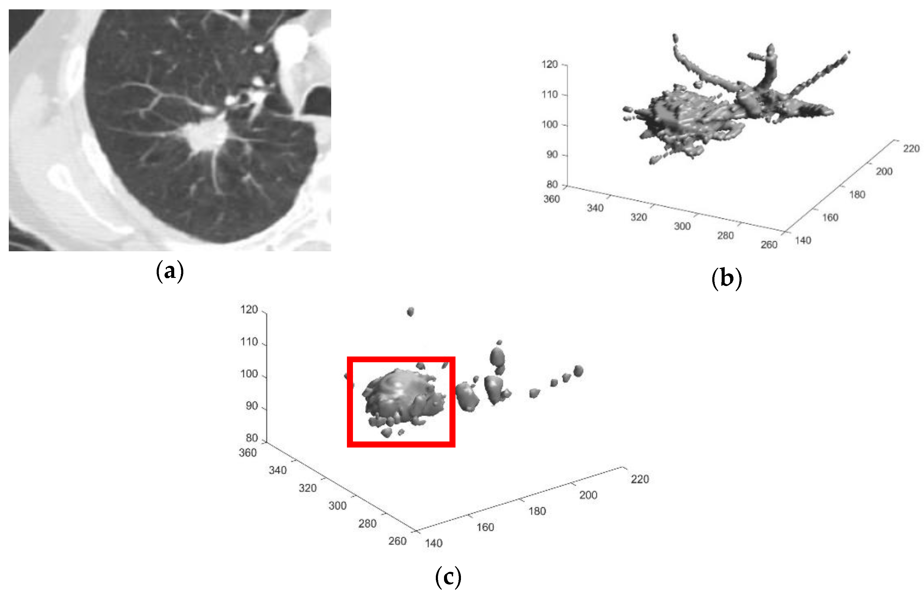
2.2.3. Preliminary Screening
2.2.4. Feature Extraction
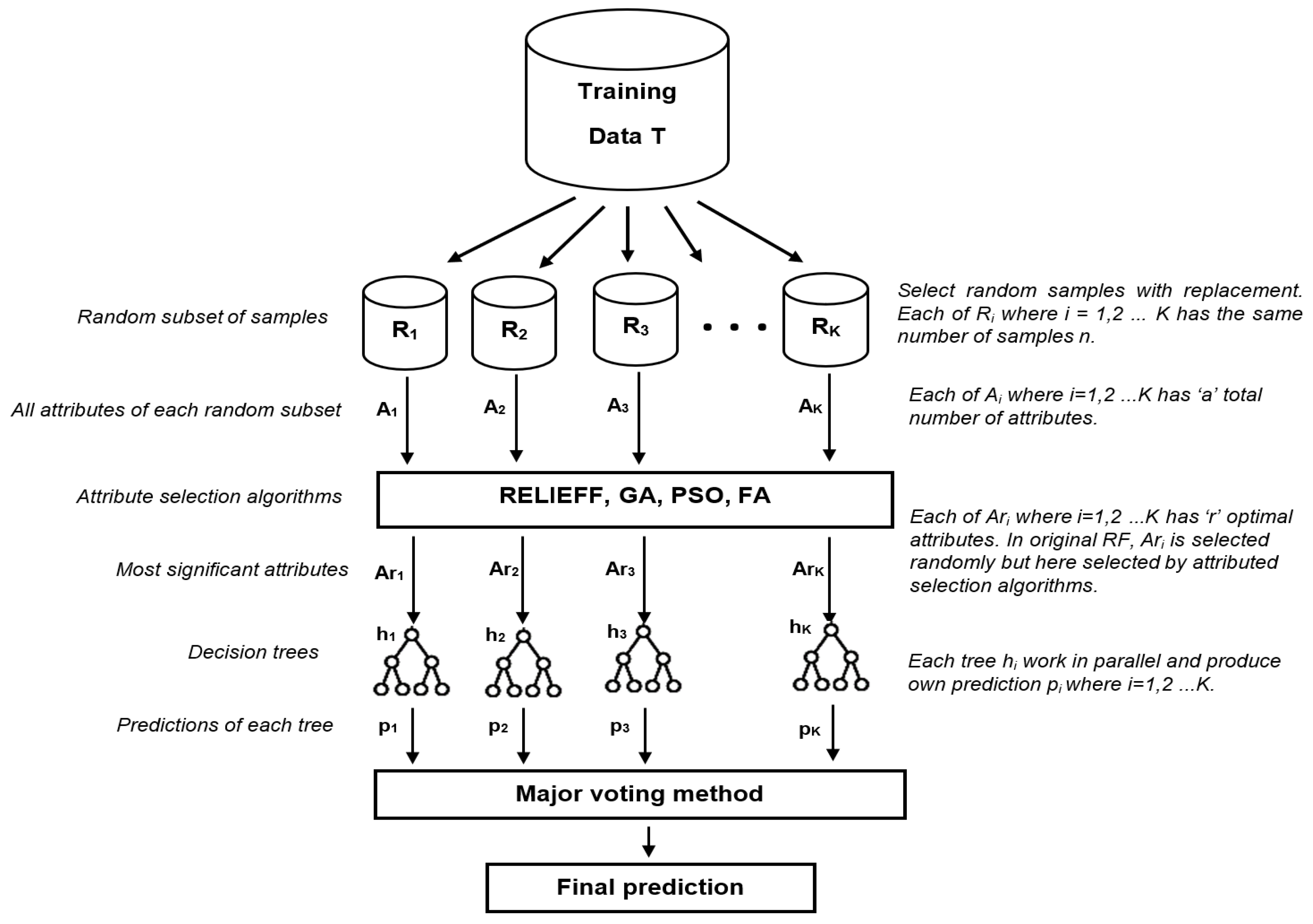
2.2.5. Improved Random Forest
3. Results and Discussions
4. Conclusions
Author Contributions
Funding
Acknowledgments
Conflicts of Interest
References
- Bray, F.; Ferlay, J.; Soerjomataram, I.; Siegel, R.L.; Torre, L.A.; Jemal, A. Global cancer statistics 2018: Globocan estimates of incidence and mortality worldwide for 36 cancers in 185 countries. CA Cancer J. Clin. 2018, 68, 394–424. [Google Scholar] [CrossRef] [PubMed]
- The National Lung Screening Trial Research Team. Reduced Lung-Cancer Mortality with Low-Dose Computed Tomographic Screening. N. Engl. J. Med. 2011, 365, 395–409. [Google Scholar] [CrossRef] [PubMed]
- Paing, M.P.; Pintavirooj, C.; Hamamoto, K.; Tungjitkusolmun, S. A study of ground-glass opacity (GGO) nodules in the automated detection of lung cancer. In Lung Cancer and Imaging; IOP Publishing: Bristol, UK, 2019; ISBN 978-0-7503-2540-0. [Google Scholar]
- Messay, T.; Hardie, R.C.; Rogers, S.K. A new computationally efficient CAD system for pulmonary nodule detection in CT imagery. Med. Image Anal. 2010, 14, 390–406. [Google Scholar] [CrossRef] [PubMed]
- Choi, W.-J.; Choi, T.-S. Genetic programming-based feature transform and classification for the automatic detection of pulmonary nodules on computed tomography images. Inf. Sci. 2012, 212, 57–78. [Google Scholar] [CrossRef]
- Shen, S.; Bui, A.A.T.; Cong, J.; Hsu, W. An automated lung segmentation approach using bidirectional chain codes to improve nodule detection accuracy. Comput. Biol. Med. 2015, 57, 139–149. [Google Scholar] [CrossRef] [PubMed]
- John, J.; Mini, M.G. Multilevel Thresholding Based Segmentation and Feature Extraction for Pulmonary Nodule Detection. Procedia Technol. 2016, 24, 957–963. [Google Scholar] [CrossRef]
- Choi, W.-J.; Choi, T.-S. Automated pulmonary nodule detection based on three-dimensional shape-based feature descriptor. Comput. Methods Programs Biomed. 2014, 113, 37–54. [Google Scholar] [CrossRef]
- Demir, Ö.; Yılmaz Çamurcu, A. Computer-aided detection of lung nodules using outer surface features. Biomed. Mater. Eng. 2015, 26, S1213–S1222. [Google Scholar] [CrossRef]
- da Silva Sousa, J.R.F.; Silva, A.C.; de Paiva, A.C.; Nunes, R.A. Methodology for automatic detection of lung nodules in computerized tomography images. Comput. Methods Programs Biomed. 2010, 98, 1–14. [Google Scholar] [CrossRef]
- Cascio, D.; Magro, R.; Fauci, F.; Iacomi, M.; Raso, G. Automatic detection of lung nodules in CT datasets based on stable 3D mass–spring models. Comput. Biol. Med. 2012, 42, 1098–1109. [Google Scholar] [CrossRef]
- Keshani, M.; Azimifar, Z.; Tajeripour, F.; Boostani, R. Lung nodule segmentation and recognition using SVM classifier and active contour modeling: A complete intelligent system. Comput. Biol. Med. 2013, 43, 287–300. [Google Scholar] [CrossRef] [PubMed]
- Zhang, W.; Wang, X.; Li, X.; Chen, J. 3D skeletonization feature based computer-aided detection system for pulmonary nodules in CT datasets. Comput. Biol. Med. 2018, 92, 64–72. [Google Scholar] [CrossRef] [PubMed]
- Yongbum, L.; Hara, T.; Fujita, H.; Itoh, S.; Ishigaki, T. Automated detection of pulmonary nodules in helical CT images based on an improved template-matching technique. IEEE Trans. Med. Imaging 2001, 20, 595–604. [Google Scholar] [CrossRef] [PubMed]
- El-Baz, A.; Elnakib, A.; Abou El-Ghar, M.; Gimel’farb, G.; Falk, R.; Farag, A. Automatic Detection of 2D and 3D Lung Nodules in Chest Spiral CT Scans. Int. J. Biomed. Imaging 2013, 2013, 1–11. [Google Scholar] [CrossRef]
- Ozekes, S.; Osman, O.; Ucan, O.N. Nodule Detection in a Lung Region that’s Segmented with Using Genetic Cellular Neural Networks and 3D Template Matching with Fuzzy Rule Based Thresholding. Korean J. Radiol. 2008, 9, 1. [Google Scholar] [CrossRef]
- Omar, A. Lung CT Parenchyma Segmentation using VGG-16 based SegNet Model. IJCA 2019, 178, 10–13. [Google Scholar] [CrossRef]
- Xu, M.; Qi, S.; Yue, Y.; Teng, Y.; Xu, L.; Yao, Y.; Qian, W. Segmentation of lung parenchyma in CT images using CNN trained with the clustering algorithm generated dataset. Biomed. Eng. Online 2019, 18, 2. [Google Scholar] [CrossRef]
- Zhang, G.; Jiang, S.; Yang, Z.; Gong, L.; Ma, X.; Zhou, Z.; Bao, C.; Liu, Q. Automatic nodule detection for lung cancer in CT images: A review. Comput. Biol. Med. 2018, 103, 287–300. [Google Scholar] [CrossRef]
- Murphy, K.; van Ginneken, B.; Schilham, A.M.R.; de Hoop, B.J.; Gietema, H.A.; Prokop, M. A large-scale evaluation of automatic pulmonary nodule detection in chest CT using local image features and k-nearest-neighbour classification. Med. Image Anal. 2009, 13, 757–770. [Google Scholar] [CrossRef]
- Tan, M.; Deklerck, R.; Jansen, B.; Bister, M. A novel computer-aided lung nodule detection system for CT images. Med. Phys. 2011, 38, 5630–5645. [Google Scholar] [CrossRef]
- Kim, D.-Y.; Kim, J.-H.; Noh, S.-M.; Park, J.-W. Pulmonary Nodule Detection using Chest Ct Images. Acta Radiol. 2003, 44, 252–257. [Google Scholar] [CrossRef] [PubMed]
- Matsumoto, S.; Ohno, Y.; Yamagata, H.; Takenaka, D.; Sugimura, K. Computer-aided detection of lung nodules on multidetector row computed tomography using three-dimensional analysis of nodule candidates and their surroundings. Radiat. Med. 2008, 26, 562–569. [Google Scholar] [CrossRef] [PubMed]
- Setio, A.A.A.; Ciompi, F.; Litjens, G.; Gerke, P.; Jacobs, C.; van Riel, S.J.; Wille, M.M.W.; Naqibullah, M.; Sanchez, C.I.; van Ginneken, B. Pulmonary Nodule Detection in CT Images: False Positive Reduction Using Multi-View Convolutional Networks. IEEE Trans. Med. Imaging 2016, 35, 1160–1169. [Google Scholar] [CrossRef] [PubMed]
- Yuan, J.; Liu, X.; Hou, F.; Qin, H.; Hao, A. Hybrid-feature-guided lung nodule type classification on CT images. Comput. Graph. 2018, 70, 288–299. [Google Scholar] [CrossRef]
- Suzuki, K.; Feng, L.; Sone, S.; Doi, K. Computer-aided diagnostic scheme for distinction between benign and malignant nodules in thoracic low-dose CT by use of massive training artificial neural network. IEEE Trans. Med. Imaging 2005, 24, 1138–1150. [Google Scholar] [CrossRef] [PubMed]
- Lee, S.L.A.; Kouzani, A.Z.; Hu, E.J. Random forest based lung nodule classification aided by clustering. Comput. Med. Imaging Graph. 2010, 34, 535–542. [Google Scholar] [CrossRef]
- Armato, S.G.; McLennan, G.; Bidaut, L.; McNitt-Gray, M.F.; Meyer, C.R.; Reeves, A.P.; Clarke, L.P. Data From LIDC-IDRI. The Cancer Imaging Archive. 2015. Available online: https://wiki.cancerimagingarchive.net/display/Public/LIDC-IDRI (accessed on 4 February 2020).
- Armato, S.G.; McLennan, G.; Bidaut, L.; McNitt-Gray, M.F.; Meyer, C.R.; Reeves, A.P.; Zhao, B.; Aberle, D.R.; Henschke, C.I.; Hoffman, E.A.; et al. The Lung Image Database Consortium (LIDC) and Image Database Resource Initiative (IDRI): A Completed Reference Database of Lung Nodules on CT Scans: The LIDC/IDRI thoracic CT database of lung nodules. Med. Phys. 2011, 38, 915–931. [Google Scholar] [CrossRef]
- Clark, K.; Vendt, B.; Smith, K.; Freymann, J.; Kirby, J.; Koppel, P.; Moore, S.; Phillips, S.; Maffitt, D.; Pringle, M.; et al. The Cancer Imaging Archive (TCIA): Maintaining and Operating a Public Information Repository. J. Digit. Imaging 2013, 26, 1045–1057. [Google Scholar] [CrossRef]
- Valente, I.R.S.; Cortez, P.C.; Neto, E.C.; Soares, J.M.; de Albuquerque, V.H.C.; Tavares, J.M.R.S. Automatic 3D pulmonary nodule detection in CT images: A survey. Comput. Methods Programs Biomed. 2016, 124, 91–107. [Google Scholar] [CrossRef]
- Adams, R.; Bischof, L. Seeded region growing. IEEE Trans. Pattern Anal. Mach. Intell. 1994, 16, 641–647. [Google Scholar] [CrossRef]
- Freeman, H. Computer Processing of Line-Drawing Images. ACM Comput. Surv. 1974, 6, 57–97. [Google Scholar] [CrossRef]
- Sánchez-Cruz, H.; López-Valdez, H.H.; Cuevas, F.J. A new relative chain code in 3D. Pattern Recognit. 2014, 47, 769–788. [Google Scholar] [CrossRef]
- Magdy, E.; Zayed, N.; Fakhr, M. Automatic Classification of Normal and Cancer Lung CT Images Using Multiscale AM-FM Features. Int. J. Biomed. Imaging 2015, 2015, 1–7. [Google Scholar] [CrossRef] [PubMed]
- Samet, H.; Tamminen, M. Efficient component labeling of images of arbitrary dimension represented by linear bintrees. IEEE Trans. Pattern Anal. Mach. Intell. 1988, 10, 579–586. [Google Scholar] [CrossRef]
- Jerman, T.; Pernuš, F.; Likar, B.; Špiclin, Ž. Beyond Frangi: An improved multiscale vesselness filter. In Proceedings of the SPIE 9413, Medical Imaging 2015: Image Processing, Orlando, FL, USA, 20 March 2015; pp. 24–26. [Google Scholar]
- Breiman, L. Random Forests. Mach. Learn. 2001, 45, 5–32. [Google Scholar] [CrossRef]
- Robnik-Šikonja, M. Improving Random Forests. In Proceedings of the Machine Learning: ECML 2004; Boulicaut, J.-F., Esposito, F., Eds.; Springer: Berlin/Heidelberg, Germany, 2004; pp. 359–370. [Google Scholar]
- Kononenko, I.; Imec, E.S.; Ikonja, M.R.-S. Overcoming the Myopia of Inductive Learning Algorithms with RELIEFF. Appl. Intell. 1997, 7, 39–55. [Google Scholar] [CrossRef]
- Oluleye, B.; Leisa, A.; Leng, J.; Dean, D. A Genetic Algorithm-Based Feature Selection. Int. J. Electron. Commun. Comput. Eng. 2014, 5, 899–905. [Google Scholar]
- Kennedy, J.; Eberhart, R. Particle swarm optimization. In Proceedings of the ICNN’95—International Conference on Neural Networks, Perth, WA, Australia, 27 November–1 December 1995; Volume 4, pp. 1942–1948. [Google Scholar]
- Yang, X.-S. Nature-Inspired Metaheuristic Algorithms, 2nd ed.; Luniver Press: Frome, UK, 2010; ISBN 978-1-905986-28-6. [Google Scholar]
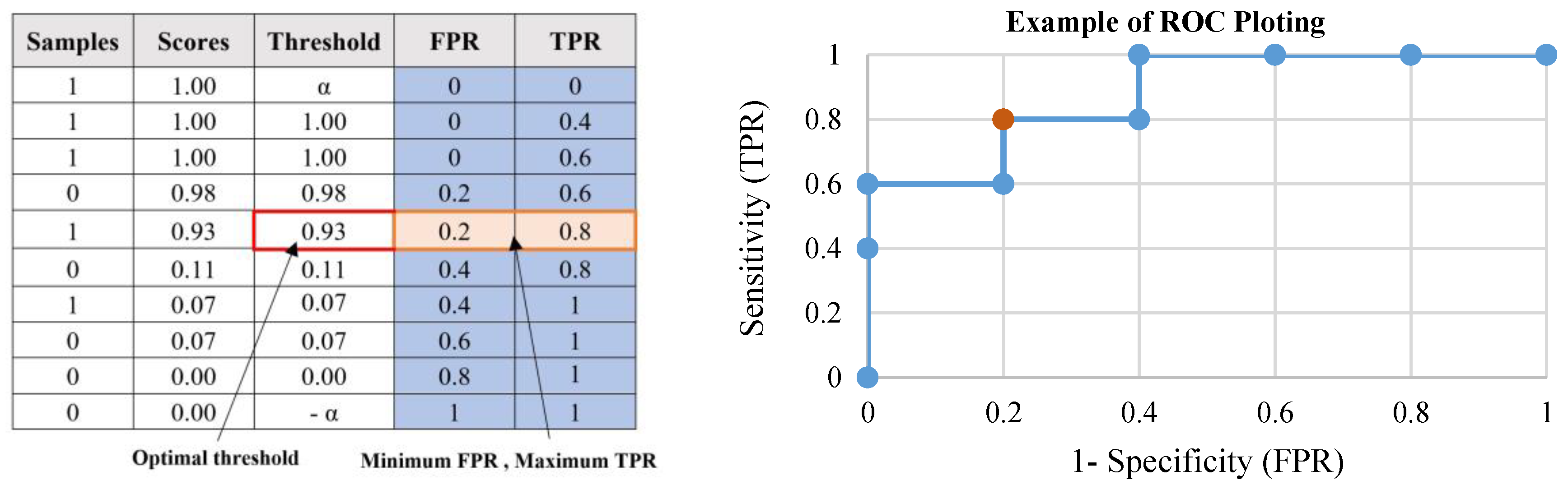
- Tharwat, A. Classification assessment methods. Appl. Comput. Inform. 2018, in press. [Google Scholar] [CrossRef]


| Features | Name | Formula |
|---|---|---|
| Geometric features (2D,3D) | Surface area | |
| Perimeter | ||
| Effective radius | ||
| Centroid | ||
| Minor axis length | ||
| Minor axis length | ||
| Elongation | ||
| Geometric features (3D) | Volume | |
| Sphericity | ||
| Compactness | ||
| Intensity and contrast features (2D, 3D) | Mean | |
| Standard deviation | ||
| Skewness | ||
| Kurtosis |
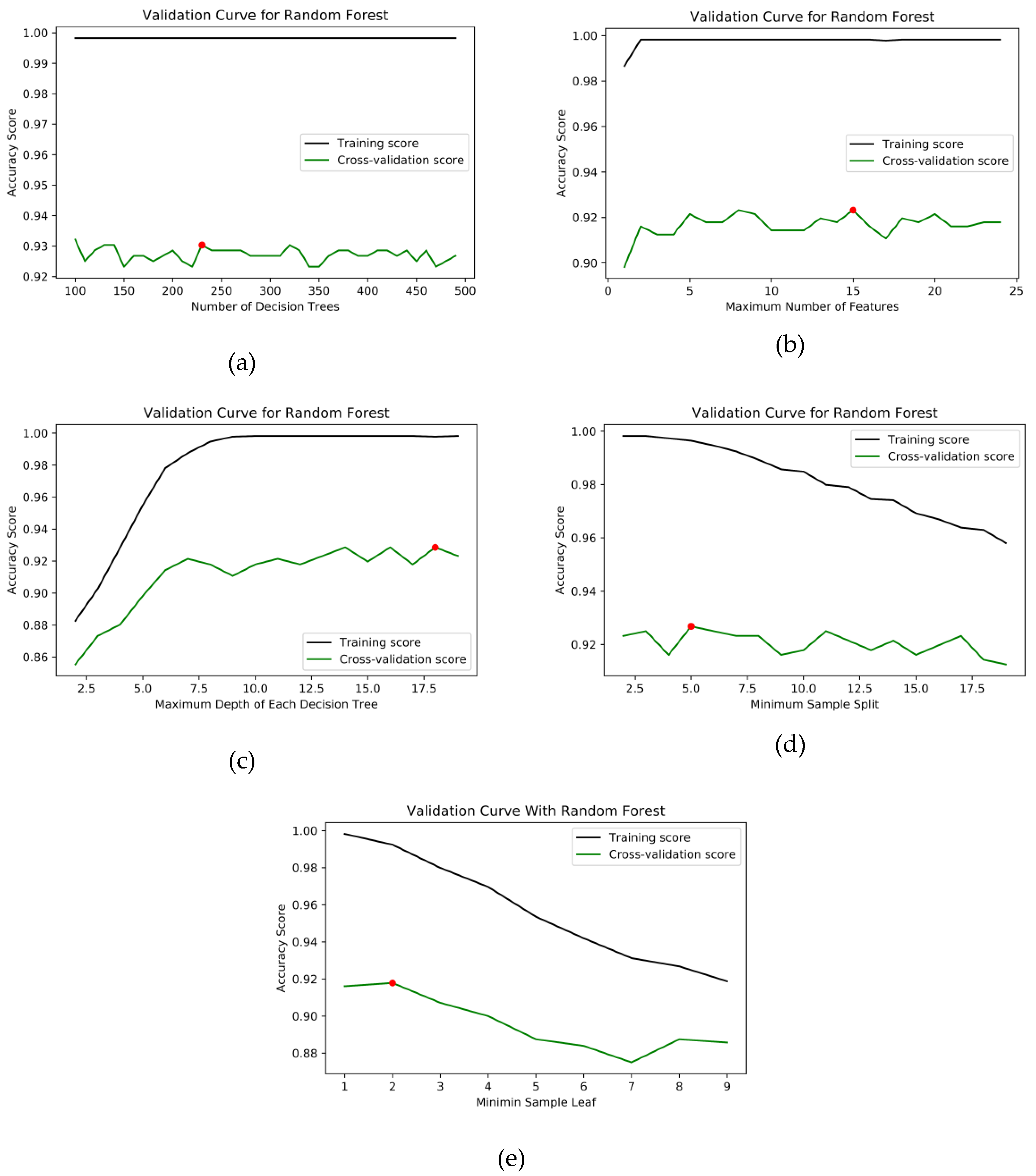
| Hyperparameter | Range | Accuracy | Selected Value |
|---|---|---|---|
| Number of decision trees | 100 to 500 | 0.9304 | 230 |
| Maximum number of features | 1 to 25 | 0.9232 | 15 |
| Maximum number of depth | 2 to 20 | 0.9285 | 18 |
| Minimum number of samples to split | 2 to 20 | 0.9267 | 5 |
| Minimum number of samples at the leaf node | 1 to 5 | 0.9178 | 2 |
| Classifiers | Assessments | Five-fold Cross-Validation | |||||
|---|---|---|---|---|---|---|---|
| Fold-1 | Fold-2 | Fold-3 | Fold-4 | Fold-5 | Mean | ||
| Original RF | Accuracy | 0.8986 | 0.9128 | 0.8899 | 0.9263 | 0.9037 | 0.9063 |
| Sensitivity | 0.8991 | 0.9358 | 0.9174 | 0.9444 | 0.8899 | 0.9173 | |
| Specificity | 0.8981 | 0.8899 | 0.8624 | 0.9083 | 0.9174 | 0.8952 | |
| False Positive | 0.1019 | 0.1101 | 0.1376 | 0.0917 | 0.0826 | 0.1048 | |
| F1-score | 0.8991 | 0.9148 | 0.8929 | 0.9273 | 0.9023 | 0.9073 | |
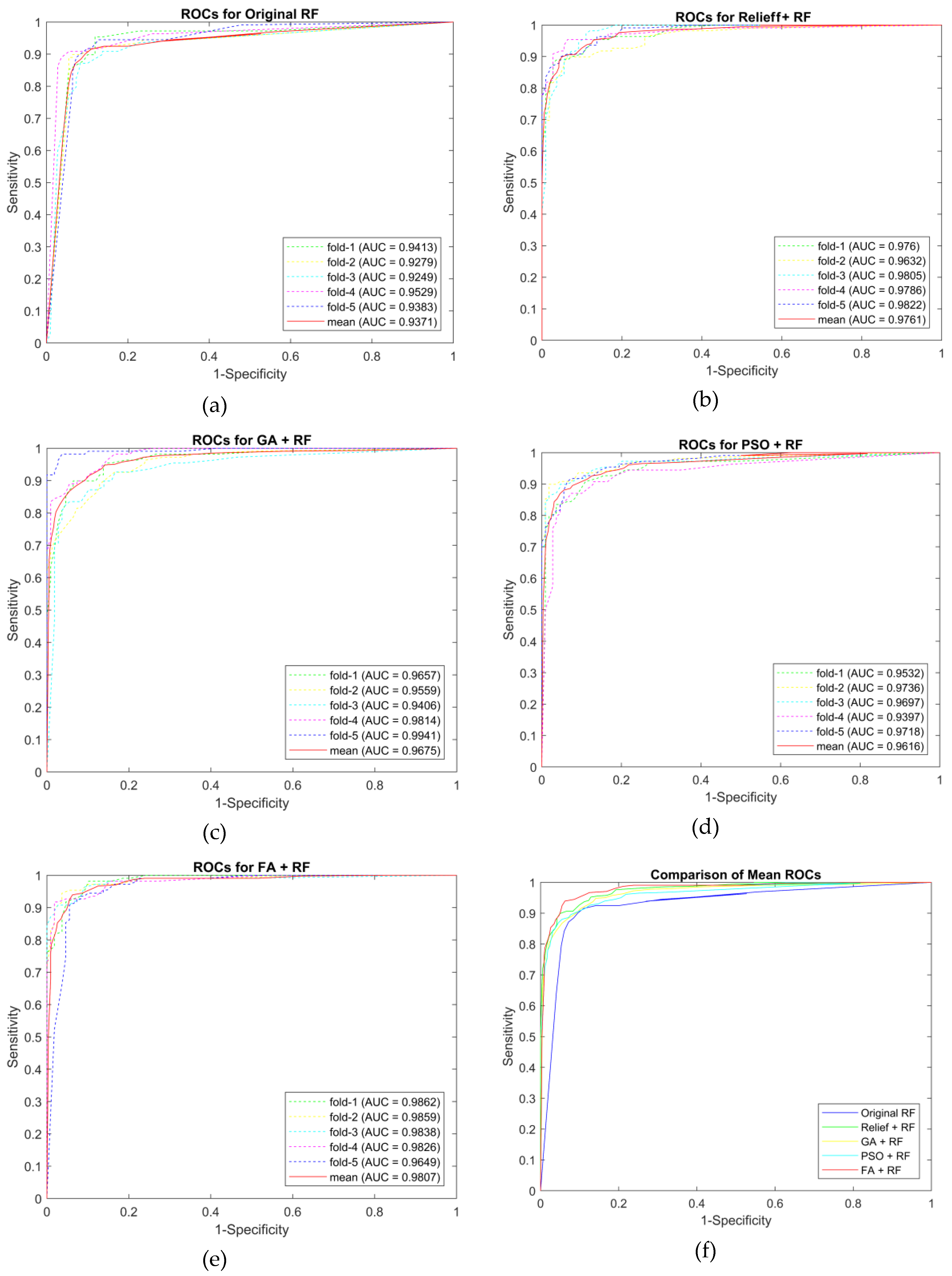
| AUC | 0.9413 | 0.9279 | 0.9249 | 0.9529 | 0.9383 | 0.9371 | |
| RELIEFF + RF | Accuracy | 0.9124 | 0.9174 | 0.9171 | 0.9358 | 0.9220 | 0.9209 |
| Sensitivity | 0.9352 | 0.9358 | 0.9174 | 0.9541 | 0.9358 | 0.9357 | |
| Specificity | 0.8899 | 0.8991 | 0.9167 | 0.9174 | 0.9083 | 0.9063 | |
| False Positive | 0.1101 | 0.1009 | 0.0833 | 0.0826 | 0.0917 | 0.0937 | |
| F1-score | 0.9140 | 0.9189 | 0.9174 | 0.9369 | 0.9231 | 0.9221 | |
| AUC | 0.9760 | 0.9632 | 0.9805 | 0.9786 | 0.9822 | 0.9761 | |
| GA + RF | Accuracy | 0.9174 | 0.9174 | 0.9124 | 0.9263 | 0.8945 | 0.9136 |
| Sensitivity | 0.9725 | 0.9725 | 0.9444 | 0.9358 | 0.9174 | 0.9485 | |
| Specificity | 0.8624 | 0.8624 | 0.8807 | 0.9167 | 0.8716 | 0.8787 | |
| False Positive | 0.1376 | 0.1376 | 0.1193 | 0.0833 | 0.1284 | 0.1213 | |
| F1-score | 0.9217 | 0.9217 | 0.9148 | 0.9273 | 0.8969 | 0.9165 | |
| AUC | 0.9646 | 0.9690 | 0.9822 | 0.9761 | 0.9729 | 0.9730 | |
| PSO + RF | Accuracy | 0.8853 | 0.9312 | 0.9174 | 0.8986 | 0.9217 | 0.9108 |
| Sensitivity | 0.9266 | 0.9633 | 0.9633 | 0.9266 | 0.9259 | 0.9411 | |
| Specificity | 0.8440 | 0.8991 | 0.8716 | 0.8704 | 0.9174 | 0.8805 | |
| False Positive | 0.1560 | 0.1009 | 0.1284 | 0.1296 | 0.0826 | 0.1195 | |
| F1-score | 0.8899 | 0.9333 | 0.9211 | 0.9018 | 0.9217 | 0.9135 | |
| AUC | 0.9532 | 0.9736 | 0.9697 | 0.9397 | 0.9718 | 0.9616 | |
| FA + RF | Accuracy | 0.9078 | 0.9539 | 0.9266 | 0.9404 | 0.9266 | 0.9311 |
| Sensitivity | 0.9630 | 0.9633 | 0.9174 | 0.9817 | 0.9174 | 0.9486 | |
| Specificity | 0.8532 | 0.9444 | 0.9358 | 0.8991 | 0.9358 | 0.9137 | |
| False Positive | 0.1468 | 0.0556 | 0.0642 | 0.1009 | 0.0642 | 0.0863 | |
| F1-score | 0.9123 | 0.9545 | 0.9259 | 0.9427 | 0.9259 | 0.9323 | |
| AUC | 0.9862 | 0.9859 | 0.9838 | 0.9826 | 0.9649 | 0.9807 | |
| Function Name | Total Time |
|---|---|
| Reading input images (Maximum: 764 slices) | 1.53 s |
| Lung regions segmentation (Automated seeded region growing) | 11.49 s |
| Border reconstruction (3D chain coding) | 99.68 s |
| Preliminary screening | 18.56 s |
| Feature extraction | 10.40 s |
| False reduction (RF+FA) | 2.74 s |
| Entire program | 144.40 s |
| References | Method | Exams | Acc (%) | Sen (%) | Spec (%) | FP (per exam) |
|---|---|---|---|---|---|---|
| [9] |
| 200 | 90.12 | 98.03 | 87.71 | 2.45 |
| [13] |
| 71 | 93.6 | 89.3 | - | 2.1 |
| [24] |
| 888 | - | 90.1 | - | 4 |
| [25] |
| 744 | 93.1 | - | - | - |
| Proposed Method |
| 888 | 93.11 | 94.86 | 91.37 | 0.0863 |
© 2020 by the authors. Licensee MDPI, Basel, Switzerland. This article is an open access article distributed under the terms and conditions of the Creative Commons Attribution (CC BY) license (http://creativecommons.org/licenses/by/4.0/).
Share and Cite
Paing, M.P.; Hamamoto, K.; Tungjitkusolmun, S.; Visitsattapongse, S.; Pintavirooj, C. Automatic Detection of Pulmonary Nodules using Three-dimensional Chain Coding and Optimized Random Forest. Appl. Sci. 2020, 10, 2346. https://doi.org/10.3390/app10072346
Paing MP, Hamamoto K, Tungjitkusolmun S, Visitsattapongse S, Pintavirooj C. Automatic Detection of Pulmonary Nodules using Three-dimensional Chain Coding and Optimized Random Forest. Applied Sciences. 2020; 10(7):2346. https://doi.org/10.3390/app10072346
Chicago/Turabian StylePaing, May Phu, Kazuhiko Hamamoto, Supan Tungjitkusolmun, Sarinporn Visitsattapongse, and Chuchart Pintavirooj. 2020. "Automatic Detection of Pulmonary Nodules using Three-dimensional Chain Coding and Optimized Random Forest" Applied Sciences 10, no. 7: 2346. https://doi.org/10.3390/app10072346
APA StylePaing, M. P., Hamamoto, K., Tungjitkusolmun, S., Visitsattapongse, S., & Pintavirooj, C. (2020). Automatic Detection of Pulmonary Nodules using Three-dimensional Chain Coding and Optimized Random Forest. Applied Sciences, 10(7), 2346. https://doi.org/10.3390/app10072346