Efficient Seismic Fragility Analysis for Large-Scale Piping System Utilizing Bayesian Approach

Abstract

In the event of an earthquake, it is essential to accurately assess the seismic fragility of piping systems to ensure the continued safety of society. When evaluating the seismic fragility of a piping system, which is generally a secondary structural system, this should mainly be an integrated model that includes both the primary structural frames and the secondary ones, unlike the primary structural system of a building. Hence, the piping seismic fragility evaluation has an issue in that it takes considerable computational time because numerical analyses must be performed on a relatively complex model. Given this background, the purpose of this study is to propose an efficient piping seismic fragility analysis method by utilizing the existing seismic fragility analysis method and the Bayesian updating concept. In order to verify the validity of the proposed method, it was applied to a building–piping coupled structural system example, and its results were analyzed and compared with the results of the existing method in terms of accuracy and efficiency. As a result, the proposed method showed a similar accuracy compared with the existing method while significantly reducing the numerical cost of nonlinear seismic response analyses necessary for these results.

1. Introduction

Recently, two earthquakes having a moment magnitude greater than 5.0 occurred in Gyeongju (2016) and Pohang (2017) on the Korean peninsula, where such strong earthquakes had been observed only rarely in the past. These earthquakes resulted in considerable damage that directly affected structural safety, causing damage such as cracks and the collapse of columns and walls that were the main structural components of buildings. In particular, the intensity of the ground motions observed in the city center (for example, USN2 of Ulsan) near the epicenter of the 2016 Gyeongju earthquake exceeded the design seismic intensity of the nuclear power plant (i.e., 0.2 g or 0.3 g-anchored USNRC R.G. 1.60 [1] design ground response spectrum) (see Figure 1). Additionally, the earthquake extensively damaged non-structural components such as ceilings and plumbing in the downtown area, threatening the safety of human life, as well as causing significant economic losses. Due to this, the perception that earthquakes might threaten the structural safety of key social infrastructure and human life has been increased in Korean society.

The post-investigation for the 1994 Northridge earthquake in the United States revealed that economic losses from damage to non-structural components accounted for more than 50% of the total economic loss induced by the earthquake [2]. Specifically, during the Northridge earthquake, failures of three plumbing lines, more than 1500 water pipelines, and 709 gas plumbing systems were reported as plumbing damage accidents, and the Olive View Medical Center in Sylmar, California, was closed. Similarly, during the 1995 Kobe earthquake in Japan, it was found that the failure of non-structural components, especially fire sprinkler piping systems, accounted for 40.8% of all failures [3]. In particular, among the non-structural components of a building, the piping system is installed and supported at several different points of the building. Due to this characteristic of the piping system, earthquake motion inputs to the support points of a piping system are different from each other, and this may cause a large displacement in the piping system. In addition, the fundamental frequency of the piping system has a value between about 1 and 10 Hz, unlike that of other non-structural components, which overlaps with the primary natural frequency of a low-rise building (F_N = 10/N Hz, N: total number of floors of a building) [4] and the concentrated frequency range of the design earthquake input motion energy (1–10 Hz). This causes a resonance effect in the piping system and ultimately increases the possibility of an even larger displacement of the piping system.

Based on this background, several researchers have conducted studies to determine the seismic safety of piping systems. Specifically, a study was conducted to investigate the limit states of T-joints [5,6], elbows [7,8], etc., which were structurally fragile components of the piping system, through a dynamic cyclic test for the piping. In addition, studies have been carried out to experimentally and analytically investigate the earthquake responses of actual piping subjected to ground shaking [9,10,11]. Based on these findings, several groups performed studies on the seismic fragility of piping systems that considered the uncertainties of earthquake loading and the piping model to assess the probabilistic seismic safety of piping [12,13,14,15]. Recently, in relation to seismically vulnerable piping systems, a study was conducted aimed at directly improving the seismic performance of piping systems by applying seismic isolators, damper devices, etc. [16,17].

On the other hand, piping systems are not usually installed alone as secondary structural systems; rather, they are supported/fixed at multiple locations on buildings, bridges, etc., which are the primary structural systems. Therefore, for the accurate seismic fragility analysis of piping systems, an integrated model that includes both primary and secondary structural frames must be established, and a coupled analysis based on the integrated model must be performed. However, such an approach has a limitation in that it requires a large computational time because numerical analyses must be performed on a relatively complex model. Thus, in the field of nuclear structural analysis and design, this is considered through a decoupled analysis. Specifically, at first, the floor response spectrum for each floor of a building is derived through seismic response analyses of the building structure, which is the primary structural system with respect to the design-input earthquake ground motion. The obtained floor response spectrum is used as the input seismic load of each support location of the piping system, which is a secondary structural system. Owing to the analytical features of this decoupled approach, the seismic response and seismic fragility analyses cannot be performed in consideration of the dynamic characteristics of an integrated model of the building and the piping system, possibly resulting in a large error that is different from the actual phenomenon. In addition, the current seismic fragility analysis method applicable to piping systems is the EPRI (Electric Power Research Institute) separation of variable (SOV) method [18,19,20,21], which basically uses the decoupled analysis approach mentioned above. This method, which is based on a linear analysis, calculates the seismic fragility by separating structure response-related variables, component response-related variables, and component capacity-related variables, and then integrating them into a single log-normal probability distribution.

Recently, in contrast to the EPRI SOV method, according to the increase in the seismic intensity, nonlinear seismic response analyses were carried out in order to directly consider the characteristics of the integrated model of a building–piping coupled structural system. Based on these analysis results, a seismic fragility analysis was conducted using the statistical technique of maximum likelihood estimation (MLE) [22,23]. However, the problem arises that a piping seismic fragility analysis based on the nonlinear seismic response analysis of the building–piping coupled numerical model requires a number of nonlinear analyses to be performed to take into account the uncertainty of the earthquake and the model, which results in a large computational cost. Accordingly, Tadinada and Gupta [24] proposed the equivalent elastic limit state (ELS) concept and related closed-form equation and developed a seismic fragility analysis method based on linear seismic response analysis and this ELS equation. Recently, Kwag and Gupta [25] proposed a novel closed-form equation by improving the accuracy of the existing ELS equation and developed an effective seismic fragility analysis method that is suitable for the secondary structural system. However, these are still seismic fragility methods based on a linear seismic analysis, and, thus, they are limited by the impossibility of deriving seismic vulnerability by accurately simulating the nonlinear behavior characteristics of the building–piping coupled structural system.

Therefore, in this study, based on the existing EPRI SOV seismic fragility analysis method, we propose an efficient piping seismic fragility analysis method using the concept of Bayesian updating. The proposed method is aimed at obtaining a piping seismic fragility curve, while not only reducing the cost of calculating nonlinear seismic response analyses, but also maintaining a similar accuracy in the results, compared to the existing MLE-based method. Specifically, to begin with, the seismic response analysis is performed on the building–piping coupled model with respect to the design earthquake loading by using the EPRI SOV method, and a prior seismic fragility curve is then derived based on this. The additional nonlinear seismic response analyses are performed based on the obtained prior seismic fragility curve, and the final seismic fragility curve is derived using the Bayesian updating technique. In order to prove the validity of the proposed method, with respect to the building–piping coupled structural model example [16], the effectiveness of the proposed method is verified by comparing the results of the proposed method with those of the existing method from the perspectives of efficiency and the accuracy. Basically, in order to increase the reliability of the numerical results of this study, the T-joint component numerical model, in which the nonlinear behavior of the piping system was concentrated, was verified using the related dynamic cyclic test results. In addition, the numerical model of the overall piping system was validated through the corresponding piping system dynamic test results. On the other hand, when dynamic testing piping systems, the experimental monitoring on the deterioration phenomena of the connections (i.e., thermal effects, prestresses, viscosity, etc.) and of the efficiency of the pipeline system (i.e., corrosion, settlements, etc.) [26,27] can be used as important information in the numerical analysis. The experience in dynamic tests showed that the variation of eigenfrequencies was not a sensible indicator of deterioration. The visual inspections could better help monitoring procedures and have been frequently used in bridges. Especially, it had been revealed that the integration of the visual inspection with the fuzzy logic treating uncertainty expressed by linguistic judgments could lead to a robust and reliable instrument [28]. It is judged that such a technique can be applied to the identification of the real state of the piping system as well.

2. Current Methods

2.1. IDA-Based MLE Method

The seismic fragility of the structural system is a conditional probability of failure according to the seismic intensity (i.e., the intensity of earthquake ground motion), which is defined as the following equation:

$$P_f\left(a\right)=P\left[D>C|a\right]$$

(1)

where a denotes the seismic intensity; C denotes the capacity of the structural system, that is, a limit state; and D denotes the dynamic seismic response at the corresponding seismic intensity input. In piping systems, C can be represented by allowable stresses, critical displacements, etc., which define the collapse of a particular piping component. Based on the defined equation, in order for the probabilistic characteristics of the earthquake loading and structural model to be taken into account, D is calculated in multiple conditions of the loading and model according to the increase in the value of seismic intensity a. Then, a conditional probability of failure is ultimately obtained by comparing such estimated values of D with C. The conditional failure probability thus obtained is called a seismic fragility curve. Here, since the dynamic seismic response analyses must be performed according to the increase in seismic intensity when calculating D, this is called an incremental dynamic analysis (IDA) method [29]. Under the IDA method framework, in order to obtain a seismic fragility curve, multiple nonlinear dynamic seismic analyses should be performed to take into account the nonlinear behavior characteristics of the structural model due to the increase in seismic input and the uncertainties of earthquake loading and structural model. Hence, the seismic fragility curve using the IDA method can be specifically expressed in the following equation:

$$P_f\left(a\right)=\frac{{\displaystyle \sum _{i=1}^{N}1\left(D\left(a_i\right)>C|a_i\right)}}{N}$$

(2)

where N is the total number of seismic response analysis simulations at a specific seismic intensity. 1 (.) is an indicator function having a value of 0 or 1. Therefore, this equation represents, at a specific seismic intensity, the ratio of the total number of simulations conducted to the number of simulations in which a failure occurs. Due to this methodological nature, the seismic fragility curve is represented by a discrete curve, and numerous nonlinear dynamic seismic analyses must be performed to obtain a complete continuous curve. However, this approach has some issues, since the cost of numerical analyses that can be performed is limited, so it is usually assumed that the seismic fragility data obtained from Equation (2) follow the cumulative log-normal probability distribution of Equation (3). Then, based on the statistical method of the MLE technique, the median A_m and log-standard deviation β of the main parameters of the log-normal probability distribution are estimated [30].

$$P_f\left(a\right)=\Phi \left[\frac{\ln \left(a\right)-\ln \left(A_m\right)}{\beta }\right]$$

(3)

Here, A_m represents the seismic intensity value for which the failure probability is 50% at the seismic fragility curve, which means the median seismic performance value of the corresponding structural system. β is the logarithmic standard deviation. The technical details on the process of estimating A_m and β are well described in the publication of Kwag et al. [31]. Based on the above descriptions and equations, the procedure for deriving the seismic fragility curve for the piping system, which is widely utilized in the current state, is briefly summarized in Figure 2. As we can see in Figure 2, the IDA-based MLE method, with respect to the seismic fragility estimation of piping systems, requires multiple nonlinear seismic response analyses; thus, this method still is limited in that it demands a substantial cost of numerical computations.

2.2. EPRI SOV Method

The seismic fragility curve of the log-normal distribution type described above can be expressed as a more detailed distribution function as follows by separately considering the randomness and the uncertainty of the input earthquake ground motion and structural model [21].

$$P_f\left(a\right)=\Phi \left[\frac{\ln \left(a/A_m\right)-{\beta }_U{\Phi }^{-1}\left(Q\right)}{{\beta }_R}\right]$$

(4)

Here, β_R and β_U are the logarithmic standard deviations indicating the randomness and the uncertainty, respectively. The parameter Q can be expressed as P [f <f′| a], which is a subjective probability (or reliability), meaning the probability that the conditional failure probability f is less than f′ at a particular seismic intensity a. The log-standard deviations of the randomness and uncertainty presented in Equation (4) can be combined into a single variable, which can be expressed as Equation (5). Based on this combined log-standard deviation, Equation (4) can be rearranged and represented as Equation (6), which finally takes the same form as Equation (3).

$${\beta }_C=\sqrt{{\beta }_R^2+{\beta }_U^2}$$

(5)

$$P_f\left(a\right)=\Phi \left[\frac{\ln \left(a/A_m\right)}{{\beta }_C}\right]$$

(6)

The parameter A_m refers to the median seismic performance value (i.e., the seismic intensity when the probability of failure is 50%) as described above, and EPRI defines it as follows by introducing the concept of the safety factor.

$$A_m=F·A_{DBE}$$

(7)

The parameter A_DBE is the seismic intensity of the design basis earthquake. The parameter F implies the safety factor of the target equipment/components/structures/systems, and this indicates the degree of margin resisting above the design basis earthquake. With regard to the piping system, this safety factor F can be further subdivided as follows, if necessary.

$$F=F_C·F_{RP}·F_{RS}$$

(8)

$${\beta }_R=\sqrt{{\beta }_{R,C}^2+{\beta }_{R,RP}^2+{\beta }_{R,RS}^2}$$

(9)

$${\beta }_U=\sqrt{{\beta }_{U,C}^2+{\beta }_{U,RP}^2+{\beta }_{U,RS}^2}$$

(10)

Here, FC refers to the capacity factor of the piping system, which is a factor indicating how much margin is greater than the defined design limit state. Especially, F_C can be further defined as F_S × F_μ. The F_S can express design margins due to design stress (strength), and F_μ can take into account design margins due to the nonlinear and inelastic behavior of structural systems. The mathematical basis of this combination is based on the feature that the median of the products of independent random variables following log-normal distributions is equal to the product of the medians of random variables [18]. Therefore, the log-normal cumulative probability distribution function, which represents the final seismic fragility, can include the nonlinear and inelastic effect and the other effects of various variables. Such an approach is in line with the way seismic fragility analysis is handled in the other studies [29,30]. Specifically, an IDA performs nonlinear and inelastic seismic response numerical analyses according to the increase in seismic intensity in consideration of the randomness and the uncertainty of the earthquake and the structural system, nonlinear and inelastic behavior of the structural system, and so on. Based on the results of these IDA analyses, the key parameters of the log-normal cumulative distribution such as A_m and β for representing the seismic fragility curve is estimated using the statistical approach. That is, the general seismic fragility analysis approach of the structural engineering treats the nonlinear and inelastic behavior effects of the structure including various other effects through a log-normal distribution function, similar to the EPRI SOV seismic fragility analysis method.

Next, F_RP refers to the response factor associated with the piping system, and F_RS refers to the response factor associated with the primary structural system supporting the piping system. These defined safety factors can be further refined by their respective characteristics. In addition, the log-standard deviations representing the randomness and the uncertainty exist individually for each defined safety factor. Such individual log-standard deviations can be integrated into a single log-standard deviation using the square root of the sum of the squares (SRSS) method, as shown in Equations (9) and (10). Due to such characteristics of this method, this is called the seismic fragility method by a variable separation. The main procedure of seismic fragility method by the variable separation aims to derive two or three main parameters that define the cumulative log-normal probability distribution of Equation (4) or Equation (6). These two or three main parameters are obtained utilizing Equations (7)–(10) based on the seismic intensity of the design basis earthquake and related safety factors. Since the EPRI SOV method is based on a linear analysis at the design basis earthquake, there may be a limit in deriving an accurate seismic fragility curve. However, as previously discussed, nonlinear numerical analysis results can be included using the F_μ factor in the EPRI SOV method.

3. Proposed Method

This subsection proposes and describes a method that can calculate a more efficient and relatively accurate piping seismic fragility curve by introducing the Bayesian updating concept based on the existing piping seismic fragility methods (i.e., (1) IDA-based MLE method and (2) EPRI SOV method). In the Bayesian updating, the seismic fragility probability model parameters are estimated using the following formulation.

$$f\left(\mathsf{\theta }|y\right)=\kappa L\left(\mathsf{\theta }|y\right)f\left(\mathsf{\theta }\right)$$

(11)

where θ = {A_m; β} represents the set of unknown parameters of the probability model of seismic fragility. y denotes the data vector of n observations y = {y₁; y₂; …, y_n}. f(θ) is a prior probability model of seismic fragility. L(θ|y) is the likelihood function that includes the information from the data vector y. f(θ|y) is the posterior probability distribution that reflects the updated state of information about the model parameter vector θ. κ is a normalizing factor as $\kappa ={({\displaystyle \int }L(\mathsf{\theta }|y)f\left(\mathsf{\theta }\right)d\mathsf{\theta }))}^{-1}$. The detailed procedures for Bayesian updates are detailed in other literature [25,32]. Figure 3 shows the main procedure of the proposed method.

First, we establish a coupled numerical model of the building–piping system. In addition, an earthquake ground motion corresponding to the seismic intensity of the design basis earthquake is defined for the building foundation. A dynamic seismic response analysis is performed based on the building–piping coupled numerical model and the input ground motion of the design basis earthquake. Based on the calculated numerical results, the first step is to derive the prior piping seismic fragility curve using the EPRI SOV seismic fragility method. The next step is to select the additional seismic intensities required to improve the accuracy of the piping seismic fragility curve based on the acquired prior fragility curve and define earthquake ground motions associated with these. Based on the selected seismic intensities, the defined ground motions are scaled and the nonlinear seismic response analyses are iteratively performed based on these scaled ground motions according to the increase of seismic intensities. Based on these numerical results, conditional failure probabilities are calculated at selected seismic intensities using Equation (2). Finally, based on the conditional failure probability information at the selected seismic intensities obtained in the previous procedure, the prior piping seismic fragility curve information is re-evaluated using the Bayesian updating concept to derive the final seismic fragility curve (so-called a posterior seismic fragility curve). As a result, the proposed approach can improve the accuracy of the existing EPRI SOV seismic fragility method through additional nonlinear seismic response analysis results. Furthermore, the cost of dynamic nonlinear numerical analyses can be minimized by using the prior seismic fragility curve information, so that the efficiency can be improved, unlike the IDA-based MLE method.

To be more specific, the IDA-based MLE method is based on the seismic fragility data obtained from the IDAs, and the key is to estimate the major variables of the cumulative probability distribution function (i.e., the cumulative log-normal distribution function) of the seismic fragility utilizing the statistical method of the MLE. As a result of such methodological features, the seismic intensity is usually divided evenly between small and large values, and the seismic fragility data is obtained in the corresponding all seismic intensities. On the other hand, the method proposed in this study efficiently derives the prior probability distribution for the seismic fragility using the EPRI SOV method at first. Next, to improve the accuracy of this prior probability distribution of the seismic fragility, additional seismic fragility data is secured. Finally, the proposed method derives the final seismic fragility probability distribution using the prior distribution and additional data within a Bayesian updating technique. Here, the proposed method could relatively save numerical costs compared to the MLE method, since additional seismic fragility data would only be needed in the seismic intensity range where the probability of failure is sensitive, unlike the MLE method.

Therefore, this approach can reduce the computational cost of nonlinear seismic response analyses and maintain a similar level of accuracy of the results, so that it is judged that the piping seismic fragility curve can be efficiently derived. From the next section on, to verify the effectiveness of the proposed piping seismic fragility method, it is applied to the example of the building–piping coupled structural system, and its results are compared with those of the existing methods in terms of accuracy and efficiency.

4. Examples

4.1. Building–Piping Coupled Structural Model

The numerical model of the building–piping coupled system used in this study was developed with OPENSEES (The Open System for Earthquake Engineering Simulation) code [33] and is constructed as shown in Figure 4. Specifically, a reinforced concrete moment resistance frame (called RC-SMRF: Special Moment Resisting Frame) was used for the building structural model. This structural model is the four-story RC-SMRF model modified from the original model [16], which was made in accordance with IBC (International Building Code) and ACI (American Concrete Institute) 318-14 [34] code by Wood et al. [35]. The model was basically designed to have five transverse bays (7.4 m long), a single longitudinal bay (9.1 m long), and the same inter-story height (3.7 m height). The main feature of this building structural model was that the sum of the moment forces acting on the column was designed to be at least 20% greater than the sum of the moment forces of the beam, according to the “strong column–weak beam design concept.” The boundary condition of the building structural model is set to have a fixed condition at the base because the building is rigidly constrained to the solid foundation. The building structural model shown in Figure 4 is a two-dimensional structural model using only a single bay, and the detailed cross-sectional information and material properties of columns and beams are described in detail in other documents [16,35].

The piping system structural model was targeted for a sprinkler piping system, for which dynamic cyclic testing was conducted as part of the “Simulation of the Seismic Performance of Nonstructural Systems” project at the University at Buffalo (UB), the State University of New York. Specifically, the utilized piping system model consists of a box-type ceiling, pedestal, vertical hangers, wire restraints, transverse sway braces, 1-inch pipe, 2-inch pipe, 4-inch pipe, etc., as shown in Figure 4. The main line and the vertical riser consist of 4-inch pipes, and the branches are composed of 1-inch and 2-inch pipes. Four-inch grooved fit joints were used for the connections for the main line and the vertical riser, and black iron threaded T-joints were used for the branch line (i.e., 1-inch and 2-inch pipes) connections. Detailed information on the layouts, material information, etc. of the piping system is provided in Tian’s literature [6].

The numerical model of the piping system basically used a linear elastic frame element, and at the connections where nonlinear behavior was predicted during an earthquake, three different types of nonlinear rotating spring elements were used for each of the 1-inch, 2-inch, and 4-inch piping joints, respectively. Specifically, the hysteretic behavior of the 1-inch-pipe T-joints is characterized by a yield strength, initial stiffness, and hardening stiffness. The isotropic hardening parameter defines the increase in the compressive/tensile yield strength as the ratio of the yield strength after the plastic deformation. The hysteretic behavior of the T-joint connection components in the 2-inch and 4-inch pipes shows the behavior of the pinched moment–rotation responses. The numerical models of the connection components were verified with the results of the dynamic cyclic test for the T-joint component [6], as shown in Figure 5. Moreover, the accuracy of the overall piping system numerical model was verified through the leakage position record of the T-joint connections of the piping system, which was observed in the dynamic test regarding the entire piping system. Figure 6 compares the observed leakage location results (“Test Leakage”) in the overall piping system during the dynamic cyclic test and the leakage location results (“Analysis Leakage”) obtained from the numerical simulations of dynamic nonlinear seismic response analyses based on the numerical piping structural model.

4.2. Seismic Response Analysis and Seismic Fragility Assessment

In this study, a time history analysis was employed as a seismic response analysis of the piping system to consider the nonlinear behaviors of the piping joint components. In the numerical model of the building–piping coupled system, a 5% damping ratio was applied to the building structural model, and a 2% damping ratio was applied to the piping system structural model. Here is the technical background for determining these damping ratios: For RC structures, the USNRC [36] recommended that the 5–7% damping ratio be used for the response prediction under strong earthquakes. In addition, most design codes and standards do not distinguish between variations in the damping ratio due to structural materials, and a 5% damping ratio is implicitly used in the seismic forces and design response spectra defined by the criteria [37]. Such damping ratio values have also been demonstrated in the measurement and various testing of damping ratios concerning the structural system subjected to the seismic load [38]. On the other hand, for piping systems, it is widely recommended to use a 2–5% damping ratio during an earthquake loading [36]. Besides, the damping ratio values for piping systems have been found to be between 2% and 5% in several tests [39,40]. Under this background, in this study, the damping ratio of the RC building structure was set at 5%, and the damping ratio of the piping system was determined to be 2%. In particular, the validity verification of the damping of the piping system was demonstrated through the piping system dynamic test results [6].

As such, due to the difference in the damping ratio between the RC structural frame and the piping, the frame–piping integrated system has a non-classical damping matrix, unlike the general structural system. In this case, the damping matrix for the entire system is constructed by assembling the damping matrix for the two subsystems: the first is for the RC structural frame and the second one is for the piping system. In these matrices, the part related to the common degree of freedom at the interface between the two subsystems includes contributions to both subsystems. The damping matrix of each numerical model of subsystems was derived by a method of the Rayleigh damping matrix generation. Based on this non-classical damping matrix, the results of the seismic response were derived at all points of the target piping system through the direct time history analysis using the Newmark method. The seismic fragility analysis of the piping system was performed based on the T-joint element responses. This numerical analysis was conducted through OPENSEES code [33], which has been proven to be accurate for the earthquake time history analysis.

To perform the piping seismic fragility analyses, a total of 21 recorded earthquake ground motions, which were proposed in the ATC-63 project [41], were utilized in this study. In order to reflect the uncertainty characteristics of the earthquake ground motion, the selected ground motion inputs included normal, reverse, and strike-slip fault phenomena, which are various fault mechanisms of earthquakes. In addition, to account for various earthquake occurrence conditions, earthquakes in various countries such as the United States, Taiwan, Japan, Iran, Turkey, etc. were selected, and less than two ground motions were only chosen regarding each earthquake. The selected ground motions were recorded from earthquakes having a moment magnitude of larger than 6.5 in all cases, and the peak ground acceleration (PGA) of the ground motions was distributed between 0.210 and 0.822 g. Detailed information on the selected ground motions such as the time series shape, response spectrum shapes, energy distribution, etc., are presented in the literature of Ryu [42]. The limit state of the piping system was defined for the T-joint where the nonlinear behavior was concentrated during an earthquake and, thus, leakage occurred. Physically, the moment when the first leakage occurred in the piping system was defined as the limit state of the piping system, which could be specified by the particular rotation angle value of the T-joint component. For the values for specific T-joint limit rotation angles, results from previous studies were used [42,43] and are briefly represented in Figure 5.

5. Results and Discussions

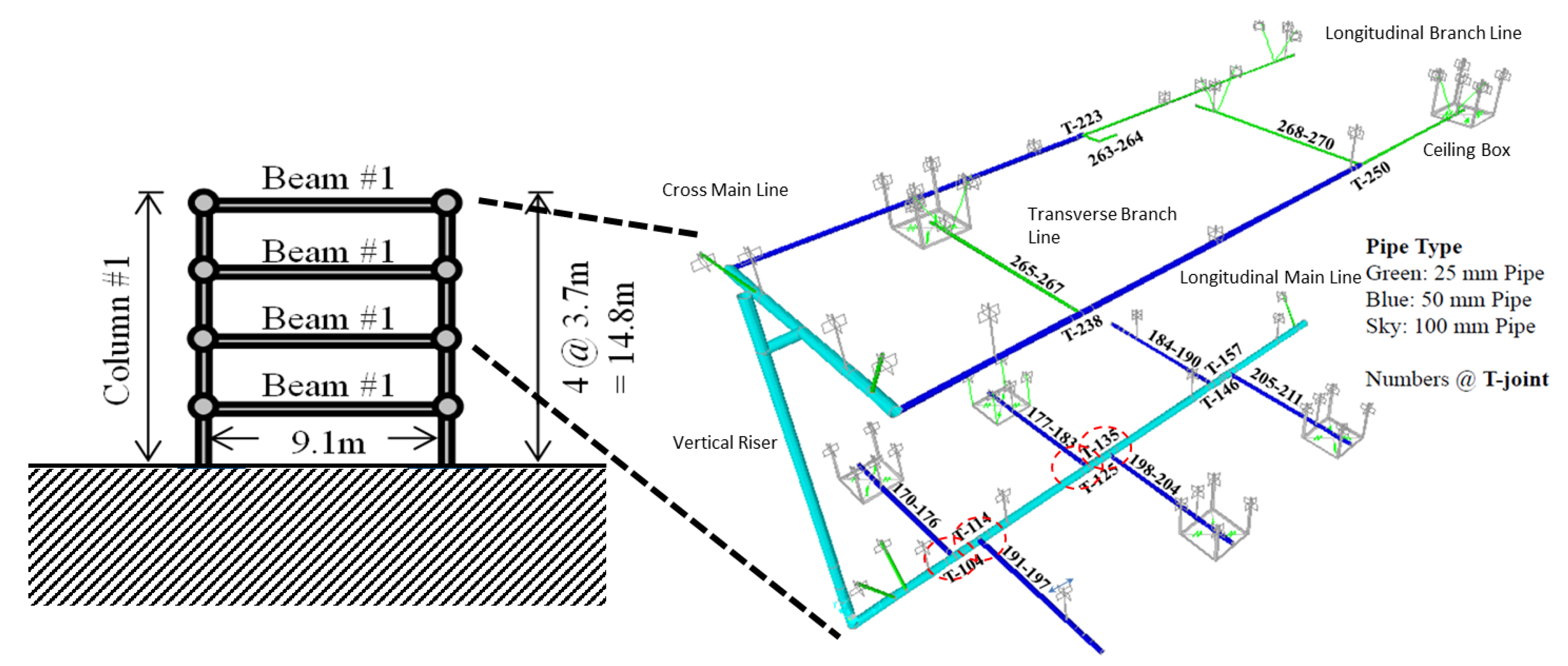
As shown in Figure 6, the main locations of seismic fragility in the piping system are considered to be the T-joints of the 2-inch pipes (e.g., T114 and T135), where leakage was observed in the dynamic cyclic test of the overall piping system. Therefore, to begin with, the seismic response analysis was performed based on the numerical model of the building–piping coupled system, and the seismic fragility of the piping system was assessed by applying the EPRI SOV method to the seismic responses of T104. When applying the EPRI SOV method, it was assumed that A_DBE, which is the seismic intensity of the design basis earthquake flowing into the foundation of the building, was set to be 0.2 g based on the seismic design regulations of the Korean building code. The seismic response analysis of the building–piping coupled numerical model subject to the ground motion corresponding to the A_DBE evaluated the maximum rotation angle response of T104 as 0.003 rad. If taking into account the calculated maximum seismic rotation angle response and 0.0135 rad, which is the limit rotation angle of the 2-inch-pipe T-joint, the safety factor F can be estimated as 4.5. Furthermore, if the uncertainty related to the piping system is assumed to be a log-standard deviation value of 0.3 using the existing piping seismic fragility research results [44], the final seismic fragility curve can be represented by the green dash-dotted line in Figure 7 (A_m = 0.9 g, β_c = 0.3).

As described above, since the EPRI SOV method cannot capture the nonlinear dynamic seismic behavior of the piping system as the seismic intensity increases, it is difficult to derive an accurate seismic fragility curve. Accordingly, the proposed method was applied to the seismic fragility analysis of the example piping system. Per the main process of the proposed method (see Figure 3), the values of the main parameters of the seismic fragility curve derived from the EPRI SOV method were utilized as the prior probability distribution information for the final fragility calculation. Specifically, the obtained prior probability distribution information was as follows: A_m~LN (0.9, 0.3) and β_c~Uniform (0.85 × 0.3, 1.15 × 0.3). Here, LN (a, b) means a log-normal probability distribution with median a and standard deviation b, and Uniform (c, d) represents a uniform probability distribution with constant values between c and d. In addition, based on this prior distribution, additional dynamic nonlinear seismic response analyses were performed at seismic intensity 0.6 and 1.2 g for further improvement of the accuracy of the seismic fragility curve. Based on these results, conditional failure probabilities were calculated at the corresponding seismic intensities. Finally, based on the Bayesian inference concept [45], the prior probability distributions of the main parameters of the seismic fragility curve obtained from the EPRI SOV method were updated to the posterior probability distributions using newly acquired conditional failure probabilities. Figure 8 shows the posterior probability distribution of the main parameters of the seismic fragility curve of T104 in the example piping system by Bayesian inference compared with the prior probability distribution. Derivation of the main parameter values of the updated posterior probability distribution based on Bayesian inference was performed by using the Metropolis–Hastings algorithm among Markov Chain Monte Carlo (MCMC) sampling techniques [46]. The total number of samples used was 10,000, among which the initial samples (also called burn-in samples) that did not satisfy the posterior probability distribution were not reflected in the parameter value calculation for the final probability distribution. Figure 9 details the MCMC sampling process that satisfies this posterior probability distribution (red big dot: an initial sample, small black points: post-samples that come after the initial sample, dotted line: the trace of the extracted samples). We represented the final updated piping seismic fragility curve through the proposed method as a solid red line in Figure 7.

To verify the piping seismic fragility analysis results of the proposed method, the IDA-based MLE method was applied to the same example piping system. For this purpose, dynamic nonlinear seismic response analyses were performed at 0.2 g intervals from 0.2 to 2.2 g seismic intensity, and the conditional failure probability information according to the defined seismic intensities was calculated based on these numerical results. The obtained conditional failure probabilities are shown discontinuously as dots in Figure 7. Based on the conditional probabilities of failure, the MLE technique was used to estimate A_m and β, which were the main variables that define the seismic fragility curve of Equation (3), and the calculated seismic fragility curve based on the estimated variable values is represented in Figure 7 as a blue dashed line. As can be seen from Figure 7, it is confirmed that the IDA-based MLE method effectively captures the discrete failure probability data obtained from the fully nonlinear seismic response analysis approach. In addition, the results of Figure 7 show that the piping seismic fragility curves obtained through the proposed method and the IDA-based MLE method are quite similar to each other. The quantitative indicators related to the accuracy comparison of the seismic fragility curves and the total number of nonlinear seismic response analyses required for the two methods are summarized and presented in

Table 1. Comparison of the accuracy and the numerical cost for the piping seismic fragility curves according to two methods, i.e., incremental dynamic analysis (IDA)-based maximum likelihood estimation (MLE) method and the proposed method (Bayesian approach with the EPRI SOV method).

Fragile Location	T104		T114		T125		T135
Method	MLE	Proposed	MLE	Proposed	MLE	Proposed	MLE	Proposed
# of nonlinear seismic analyses	231 (=11 × 21)	43 (=1 + 2 × 21)	231 (=11 × 21)	43 (=1 + 2 × 21)	231 (=11 × 21)	43 (=1 + 2 × 21)	231 (=11 × 21)	43 (=1 + 2 × 21)
R2	0.986	0.984	0.987	0.990	0.990	0.991	0.993	0.994
RMSE	0.045	0.049	0.039	0.033	0.036	0.036	0.030	0.036

. The quantitative comparison of the accuracy of seismic fragility curve results was carried out by comparing the R2 and root mean squared error (RMSE) values. It should be noted that the IDA-based MLE method performed 231 (=11 × 21) nonlinear seismic response analyses regarding the 21 earthquake ground motions in the total 11 seismic intensities to calculate the final piping seismic fragility curve. On the other hand, the proposed method conducted a single seismic response analysis for the EPRI SOV method and additionally performed nonlinear seismic response analyses in the ground motion inputs of 0.6 g and 1.2 g seismic intensity, respectively; thus, a total of 43 (=1 + 2 × 21) numerical simulations were made.

To be more specific, in the numerical example used in this study, the IDA-based MLE method, evenly divided the seismic intensities into 0.2 g intervals from 0.2 to 2.2 g and considered the uncertainty of the earthquake loadings to a total of 21 recorded ground motions; thus, this method finally made use of a total of 231 numerical analyses. On the other hand, the method proposed in this study used the EPRI SOV method to estimate the prior seismic fragility distribution in the first place. Here, the EPRI SOV method used only the results of a single numerical analysis regarding the design seismic load that satisfied the design criteria in order for estimating such seismic fragility distribution. The proposed method secured seismic fragility data only in the 0.6 g and 1.2 g seismic intensity where the probability of failure is sensitive, based on this prior seismic fragility distribution. Finally, this method calculated the final seismic fragility curve using the additional data and the Bayesian updating technique. Here, because the proposed method further considered each of the 21 ground motions at the two seismic intensities (i.e., 0.6 g and 1.2 g), the total number of final numerical analyses conducted was 43. In conclusion, the proposed method showed similar accuracy compared with the existing IDA-based MLE method in terms of seismic fragility results, but it reduced the numerical simulation cost of nonlinear seismic response analyses considerably. These numerical example results are a single case study of the efficiency of the proposed method compared to the current MLE approach, and the specific values related to this example may vary depending on the degree of segmentation in the seismic intensities, the number of the earthquake ground motion records, and so on. However, unlike the MLE approach, the proposed method can minimize the number of seismic fragility data required by utilizing the prior probability distribution; thus, this can be expected to achieve the efficiency in most case studies relatively compared to the current approach.

The overall process of the seismic fragility assessment applied to the limit state of T104 in the piping system described above was similarly applied to the remaining seismically vulnerable piping components (i.e., T114, T125, and T135). The obtained piping seismic fragility curve results for these components are presented in Figure 10, Figure 11, and Figure 12, respectively. Moreover, the quantitative indicators related to the accuracy comparison of the piping seismic fragility curves for T114, T125, and T135, and the total number of nonlinear seismic response analyses required are summarized in Table 1 together with the results regarding T104. As can be seen from the figures and the table, the proposed method applied to T114, T125, and T135 also can be confirmed to be more efficient in that it obtains piping seismic fragility curves with similar accuracy while reducing the numerical cost of nonlinear seismic response analyses.

6. Summary and Conclusions

In this study, a method for efficiently estimating the seismic fragility of the piping system was presented. Specifically, based on the existing EPRI SOV seismic fragility analysis method, we proposed an approach to calculate the piping seismic fragility curve using the concept of Bayesian inference. This method acquires the prior piping seismic fragility curve through the EPRI SOV method and minimizes the numerical cost of nonlinear seismic response analyses required for the accurate seismic fragility curve calculation using the obtained prior probability distribution and Bayesian updating concept. Ultimately, this approach creates an efficient process of performing the piping seismic fragility calculation that reduces the cost of calculating the required nonlinear seismic response analyses compared to the conventional IDA-based MLE method, while maintaining the accuracy of the fragility results.

In order to verify the validity of the proposed method, piping seismic fragility curves were calculated by applying the proposed method to the example of the building–piping coupled structural system. The consideration of the damping ratio for the coupled structural model was done by constituting the non-classical damping matrix because the damping ratios of each subsystem are different from each other. Such a non-classical damping matrix was considered in the process of the earthquake time history analyses. Specifically, the piping seismic fragility curve results to which the proposed method was applied were compared with the results of the existing IDA-based MLE method and were analyzed in terms of accuracy and efficiency. As a result, the method proposed in this study showed similar accuracy compared with the existing method regarding the final seismic fragility results, but it reduced the numerical cost of nonlinear seismic response analyses. Therefore, the method proposed in this study and related research results can be judged as being an effective method for analyzing the seismic fragility of large piping systems in the future.

References

1. USNRC RG 1.60. Design Response Spectra for Seismic Design of Nuclear Power Plants; Rev. 2; U.S. Nuclear Regulatory Commission: Washington, DC, USA, 2014.
2. Kircher, C.A. It makes dollars and sense to improve nonstructural system performance. In Proceedings of the Atc 29-2 Seminar on Seismic Design, Performance, and Retrofit of Nonstructural Components in Critical Facilities, Newport Beach, CA, USA, 23–24 October 2003. [Google Scholar]
3. Sekizawa, A.; Ebihara, M.; Notake, H. Development of seismic-induced fire risk assessment method for a building. In Proceedings of the Seventh International Symposium on Fire Safety Science, Worcester, MA, USA, 16–21 June 2002; pp. 309–320. [Google Scholar]
4. ASCE/SEI 7-16. Minimum Design Loads for Buildings and Other Structures; American Society of Civil Engineers: Alexander Bell Drive Reston, WV, USA, 2017. [Google Scholar]
5. Ju, B.-S.; Tadinada, S.K.; Gupta, A. Fragility analysis of threaded tee-joint connections in hospital piping systems. In Proceedings of the ASME 2011 Pressure Vessels and Piping Conference, Baltimore, MD, USA, 17–21 July 2011. [Google Scholar]
6. Tian, Y. Experimental Seismic Study of Pressurized Fire Sprinkler Piping Subsystems. Ph.D. Thesis, State University of New York at Buffalo, New York, NY, USA, 2013. [Google Scholar]
7. Jeon, B.G.; Kim, S.W.; Choi, H.S.; Park, D.U.; Kim, N.S. A failure estimation method of steel pipe elbows under in-plane cyclic loading. Nucl. Eng. Technol. 2017, 49, 245–253. [Google Scholar] [CrossRef] [Green Version]
8. Kim, S.W.; Choi, H.S.; Jeon, B.G.; Hahm, D.G. Low-cycle fatigue behaviors of the elbow in a nuclear power plant piping system using the moment and deformation angle. Eng. Fail. Anal. 2019, 96, 348–361. [Google Scholar] [CrossRef]
9. Hahm, D.; Park, J.; Choi, I.K. Seismic performance evaluation of piping system crossing the isolation interface in seismically isolated NPP. J. Earthq. Eng. Soc. Korea 2014, 18, 141–150. [Google Scholar] [CrossRef]
10. Tian, Y.; Filiatrault, A.; Mosqueda, G. Seismic response of pressurized fire sprinkler piping systems I: experimental study. J. Earthq. Eng. 2015, 19, 649–673. [Google Scholar] [CrossRef]
11. Tian, Y.; Filiatrault, A.; Mosqueda, G. Seismic response of pressurized fire sprinkler piping systems II: numerical study. J. Earthq. Eng. 2015, 19, 674–699. [Google Scholar] [CrossRef]
12. Ju, B.S.; Jung, W.Y.; Ryu, Y.H. Seismic fragility evaluation of piping system installed in critical structures. Struct. Eng. Mech. 2013, 46, 337–352. [Google Scholar] [CrossRef]
13. Ju, B.S.; Gupta, A. Seismic fragility of threaded Tee-joint connections in piping systems. Int. J. Press. Vessel. Pip. 2015, 132, 106–118. [Google Scholar] [CrossRef]
14. Soroushian, S.; Zaghi, A.E.; Maragakis, M.; Echevarria, A.; Tian, Y.; Filiatrault, A. Analytical seismic fragility analyses of fire sprinkler piping systems with threaded joints. Earthq. Spectra 2015, 31, 1125–1155. [Google Scholar] [CrossRef]
15. Kim, S.W.; Jeon, B.G.; Hahm, D.G.; Kim, M.K. Seismic fragility evaluation of the base-isolated nuclear power plant piping system using the failure criterion based on stress-strain. Nucl. Eng. Technol. 2019, 51, 561–572. [Google Scholar] [CrossRef]
16. Ryu, Y.; Kwag, S.; Ju, B.S. Fragility assessments of multi-story piping systems within a seismically isolated low-rise building. Sustainability 2018, 10, 3775. [Google Scholar] [CrossRef] [Green Version]
17. Kwag, S.; Kwak, J.; Lee, H.; Oh, J.; Koo, G.H. Enhancement in the seismic performance of a nuclear piping system using multiple tuned mass dampers. Energies 2019, 12, 2077. [Google Scholar] [CrossRef] [Green Version]
18. EPRI. Methodology for Developing Seismic Fragilities; TR-103959; Electric Power Research Institute: Palo Alto, CA, USA, 1994. [Google Scholar]
19. EPRI. Seismic Fragility Application Guide; No.1002988; Electric Power Research Institute: Palo Alto, CA, USA, 2002. [Google Scholar]
20. EPRI. Seismic Fragility Applications Guide Update; No.1019200; Electric Power Research Institute: Palo Alto, CA, USA, 2009. [Google Scholar]
21. EPRI. Seismic Fragility and Seismic Margin Guidance for Seismic Probabilistic Risk Assessments; No.3002012994; Electric Power Research Institute: Palo Alto, CA, USA, 2018. [Google Scholar]
22. Ju, B.S.; Gupta, A.; Ryu, Y.H. Piping fragility evaluation: Interaction with high-rise building performance. J. Press. Vessel Technol. 2017, 139, 031801. [Google Scholar] [CrossRef]
23. Ryu, Y.; Gupta, A.; Ju, B.S. Fragility evaluation in building-piping systems: Effect of piping interaction with buildings. J. Press. Vessel Technol. 2019, 141, 010906. [Google Scholar] [CrossRef]
24. Tadinada, S.K.; Gupta, A. Structural fragility of T-joint connections in large-scale piping systems using equivalent elastic time-history simulations. Struct. Saf. 2017, 65, 49–59. [Google Scholar] [CrossRef]
25. Kwag, S.; Gupta, A. Computationally efficient fragility assessment using equivalent elastic limit state and Bayesian updating. Comput. Struct. 2018, 197, 1–11. [Google Scholar] [CrossRef]
26. Sundaram, A.; Kesavan, K.; Parivallal, S. Recent advances in health monitoring and assessment of in-service oil and gas buried pipelines. J. Inst. Eng. (India) 2018, 99, 729–740. [Google Scholar] [CrossRef]
27. Porcu, M.C.; Patteri, D.M.; Melis, S.; Aymerich, F. Effectiveness of the FRF curvature technique for structural health monitoring. Constr. Build. Mater. 2019, 226, 173–187. [Google Scholar] [CrossRef]
28. Mistretta, F.; Piras, M.V.; Fadda, M.L. A reliable visual inspection method for the assessment of r.c. structures through fuzzy logic analysis. In Proceedings of the 4th International Symposium on Life-Cycle Civil Engineering (IALCCE2014), Tokyo, Japan, 16–19 November 2014; pp. 1154–1160. [Google Scholar]
29. Vamvatsikos, D.; Cornell, C.A. Incremental dynamic analysis. Earthq. Eng. Struct. Dyn. 2002, 31, 491–514. [Google Scholar] [CrossRef]
30. Shinozuka, M.; Feng, M.Q.; Kim, H.K.; Kim, S.H. Nonlinear static procedure for fragility curve development. J. Eng. Mech. 2000, 126, 1287–1295. [Google Scholar] [CrossRef] [Green Version]
31. Kwag, S.; Ju, B.; Jung, W. Beneficial and detrimental effects of soil-structure interaction on probabilistic seismic hazard and risk of nuclear power plant. Adv. Civ. Eng. 2018, 2018, 2698319. [Google Scholar] [CrossRef]
32. Andreini, M.; Gardoni, P.; Pagliara, S.; Sassu, M. Probabilistic models for the erosion rate in embankments and reliability analysis of earth dams. Reliab. Eng. Syst. Saf. 2019, 181, 142–155. [Google Scholar] [CrossRef]
33. OpenSees (Open System for Earthquake Engineering Simulation). Available online: heep://opensees.berkeley.edu/ (accessed on 1 December 2019).
34. ACI 318-14. Building Code Requirements for Structural Concrete; American Concrete Institute: Farmington Hills, MI, USA, 2014. [Google Scholar]
35. Wood, R.L.; Hutchinson, T.C.; Lee, C.; Grigoriu, M.D. Fragility Function Development for Nonstructural Component Systems; Technical Report; Structural Engineering and Earthquake Simulation Laboratory: New York, NY, USA, 2012. [Google Scholar]
36. USNRC RG 1.61. Damping Values for Seismic Design of Nuclear Power Plants; Rev. 1; U.S. Nuclear Regulatory Commission: Washington, DC, USA, 2007.
37. Chopra, A.K. Dynamics of Structures, 5th ed.; Pearson Prentice Hall: Upper Saddle River, NJ, USA, 2017. [Google Scholar]
38. Papagiannopoulos, G.; Beskos, D. Damping identification for building structures subjected to earthquakes: A review. J. Serb. Soc. Comput. Mech. 2012, 6, 129–147. [Google Scholar]
39. Wigaard, J.; Hoen, C.; Fredö, C.R. Designing structural damping to avoid resonance problems in structures, piping and subsea equipment: Risk reduction and fatigue life improvement. In Proceedings of the 24th International Conference on Offshore Mechanics and Arctic Engineering (OMAE 2005-67456), Halkidiki, Greece, 12–17 June 2005; pp. 925–932. [Google Scholar]
40. Nie, J.; Morante, R.J.; Hofmayer, C.H.; Ali, S.A. Assessing Equivalent Viscous Damping Using Piping System Test Results. In Proceedings of the ASME 2010 Pressure Vessels and Piping Division/K-PVP Conference (PVP2010-25465), Washington, DC, USA, 18–22 July 2010; pp. 249–255. [Google Scholar]
41. FEMA. Quantification of Building Seismic Performance Factors; Report No. P695; Federal Emergency Management Agency: Washington, DC, USA, 2009.
42. Ryu, Y. Fragility of Piping Systems and Reliability of Piping Components. Ph.D. Thesis, North Carolina State University, Raleigh, NC, USA, 2013. [Google Scholar]
43. Ju, B. Seismic Fragility of Piping System. Ph.D. Thesis, North Carolina State University, Raleigh, NC, USA, 2011. [Google Scholar]
44. EPRI. Seismic Probabilistic Risk Assessment Implementation Guide; No.3002000709; Electric Power Research Institute: Palo Alto, CA, USA, 2013. [Google Scholar]
45. Gelman, A.; Carlin, J.B.; Stern, H.S.; Dunson, D.B.; Vehtari, A.; Rubin, D.B. Bayesian Data Analysis; Chapman and Hall/CRC: New York, NY, USA, 2013. [Google Scholar]
46. Kwag, S.; Ju, B.S. Application of a Bayesian hierarchical model to system identification of structural parameters. Eng. Comput. 2019. In Press. [Google Scholar] [CrossRef]
Figure 1. Comparison between the response spectra obtained from ground motions at the observation posts of USN2 (Ulsan), DKJ (Deokjeongli), and MKL (Myeongkaeli) measured in the 2016 Gyeongju earthquake and the design response spectrum of USNRC RG 1.60.
Applsci 10 01515 g001
Figure 2. Process used for piping seismic fragility evaluation of incremental dynamic analysis (IDA)-based maximum likelihood estimation (MLE) method.
Applsci 10 01515 g002
Figure 3. Proposed process of the piping seismic fragility evaluation based on the EPRI (Electric Power Research Institute) separation of variable (SOV) method and Bayesian updating.
Applsci 10 01515 g003
Figure 4. Building–piping coupled structural model.
Applsci 10 01515 g004
Figure 5. Piping T-joint numerical model validation: (a) dynamic cyclic test of 2-inch piping T-joint component; (b) 1-inch, 2-inch and 4-inch joint numerical model verification results.
Applsci 10 01515 g005
Figure 6. Numerical model validation of two-story piping system: (a) dynamic test for two-story sprinkler piping system; (b) piping system numerical model verification result.
Applsci 10 01515 g006
Figure 7. Piping seismic fragility curve regarding a limit state of seismically vulnerable T-joint T104.
Applsci 10 01515 g007
Figure 8. Distribution of main parameters for piping seismic fragility curve (regarding the limit state of T104): (a) a prior probability distribution and (b) a posterior probability distribution.
Applsci 10 01515 g008
Figure 9. The posterior distribution of main parameters for piping seismic fragility curve (regarding the limit state of T104), and the related Markov Chain Monte Carlo (MCMC) sampling process.
Applsci 10 01515 g009
Figure 10. Piping seismic fragility curve regarding a limit state of seismically vulnerable T-joint T114.
Applsci 10 01515 g010
Figure 11. Piping seismic fragility curve regarding a limit state of seismically vulnerable T-joint T125.
Applsci 10 01515 g011
Figure 12. Piping seismic fragility curve regarding a limit state of seismically vulnerable T-joint T135.
Applsci 10 01515 g012