A Simple Mono-Dimensional Approach for Lap Time Optimisation

Abstract

Lap time minimisation methods have great relevance in the analysis of race tracks, and in the design and optimisation of race vehicles. Several lap time minimisation approaches have been proposed in the literature, which are computationally demanding because they need to either solve differential equations or to implement a forward–backward integration based on an apex-finding method. This paper proposes an alternative method, based on a mono-dimensional quasi-steady-state numerical approach. The proposed approach uses a simplified vehicle model accounting for combined tyre–road interactions, aerodynamic effects, and power limitations. The method exploits the knowledge of the curvature of the trajectory, which is worked out through a rigorous approach that allows for the use trajectories defined with respect to ageneric curve parameter and not necessarily the arc length. An iterative routine is implemented that exploits the vehicle dynamics, without solving differential equations or performing forward–backward integrations from the trajectory apexes. Simulations are carried out on three different tracks and are shown to be computationally efficient. Despite being intentionally simple, the proposed method allows to grasp key aspects of the problem, such as the effect of the combined tyre–road interactions on the acceleration profiles, and the effect of aerodynamic drag and downforce on the position of the braking point on the track and on the speed profile.

1. Introduction

Race car drivers are expected to achieve a minimum lap time by exploiting all of the grip potential of a given vehicle [1,2,3]. Given a driving track, the driver should make optimal use of the available control inputs, mainly including the accelerator and brake pedal positions, along with the steering wheel angle. Minimum lap time strategies have been investigated for more than 60 years [4]. They are very challenging problems, but with potentially very wide applications, including the analysis of race tracks (e.g., Formula 1) from the point of view of the human drivers and track engineers, the optimisation of vehicle design/setup, and the potential combination of advanced vehicle control techniques [5].

The most common methods for lap time simulation are [6]: (i) optimal control problem (OCP) approaches; and (ii) quasi-steady-state (QSS) approaches. Optimal control is used when the trajectory is not known a priori. This might be the case when it is necessary to find the optimal trajectory, e.g., the first time a track is studied or simply when the track is new, as it sometimes happens, even in Formula 1. OCPs are approachable either with direct methods (which solve the problem using nonlinear programming (NLP) techniques [7,8]) or with indirect methods (which solve the problem using numerical techniques for systems of differential equations [9,10]). The key peculiarities of the direct and indirect methods have been extensively discussed in the literature [11]. QSS methods, instead, rely on a given trajectory. They are based on steady-state vehicle dynamics equations, with the exception of the vehicle speed. Normally, the path is divided into small segments and the corner apexes are identified; hence, the maximum vehicle speed is therein calculated. The acceleration and braking zones are worked out by forward and backward integration, respectively, after and before each apex, and the speed profiles between the apexes are connected at their intersection points [12]. While integrating backwards, the maximum braking capabilities are considered, which normally include grip and aerodynamic effects. On the other hand, forward integration accounts for the maximum acceleration capabilities, which may include grip, aerodynamics, and power limits. In the literature [13], a method is proposed that employs QSS models and free trajectory using a vehicle g–g map, and then applying the OCP techniques again. Further simulation studies have been proposed to investigate additional aspects, including the extension of QSS methods to transients [14,15] and modelling three-dimensional roads [16].

In terms of computational cost, both OCP and QSS are generally quite demanding. This is because of the solution of differential equations through direct/indirect methods (OCP) and the backward/forward integration from each apex (QSS), respectively. In the analysis of OCP techniques in reference [11], the authors suggested that new methods should be investigated that "have the ability to compute a simulation in a reasonable amount of time, e.g., less than a few hours". For example, the OCP method in reference [17] took around 8 hours to simulate a full lap of the Jerez circuit. QSS methods are generally faster than the OCP ones. The QSS method in reference [12] took 16 minutes to simulate the Barcelona circuit, compared with 39.8 hours using the OCP method in reference [18]. Still, that is around 5–10 times (depending on the vehicle) the actual lap time. In addition, the authors of the QSS technique in reference [19] stated that their method is "for design phase decisions but not for a fast trackside usage".

In this paper, a new QSS approach is proposed for fixed trajectories. It is based on a numerical method using a simplified vehicle model including physical constraints, such as combined tyre–road interaction limits, aerodynamic effects, and engine power boundaries. The main advantage of the proposed method lies in the low computational cost. The reason for this is that there is no need for solutions of differential equations (as in standard OCP methods), nor backward/forward integrations in order to work out the optimal speed profiles (as in standard QSS methods). The proposed method exploits the knowledge of the curvature of the trajectory. The curvature is worked out through a rigorous approach, with the benefit that it allows for the use of trajectories defined with respect to a generic curve parameter and not necessarily the arc length. Simulations are carried out along a circle, an ellipse, and a combination of straight lines and a hairpin bend.

The remainder of the paper is structured as follows. Section 2 discusses the modelling of the vehicle and its performance limits. Section 3 describes the proposed optimisation approach. The simulation results are in Section 4. The main conclusions are drawn in Section 5.

2. Vehicle Modelling and Performance Bounds

This paper focuses on mono-dimensional tracks, i.e., predefined trajectories. Let $\lambda$ be a generic parameter. Given a curve $\gamma \left(\lambda \right)$, which may or may not be closed, the vehicle negotiating $\gamma \left(\lambda \right)$ will be represented as a mass point that moves along the curve, similar to [20]. The curve can also be expressed as a function of the arc length (curvilinear abscissa), $s$, as $\gamma \left(s\left(\lambda \right)\right)$. A condition that needs to be fulfilled is that the car is always on the track, i.e.,

$$x\left(\mathsf{\lambda }\right)\equiv \gamma \left(s\left(\mathsf{\lambda }\right)\right)$$

(1)

where $x\left(\lambda \right)$ is the position vector with respect to a fixed arbitrary reference frame. Once the curve is assigned, together with the initial conditions, one can determine the optimal law of the driver’s behaviour on the accelerator and brake pedals, as functions of the position on the track, so as to minimise the time to cover $\gamma \left(s\left(\lambda \right)\right)$:

$$\underset{a_x\left(s\right)}{\min }\int \frac{1}{v\left(a_x\left(s\right)\right)}\mathrm{d}s\hspace{1em}\mathrm{subject}\mathrm{to}\hspace{1em}\Vert a_x\left(s\right)\Vert \le h\left(a_y\left(s\right),v\left(a_x\left(s\right)\right)\right)$$

(2)

where $h$ represents the physical constraints or performance bounds, $a_y$ is the lateral acceleration, and $v=\dot{s}$ is the vehicle speed. $h$ depends on both the grip and engine power.

The mathematical modelling of the physical constraints was designed so as to capture the most relevant aspects of road dynamics. Three main factors were considered, namely:

• Adherence of tyres to the asphalt (grip);
• Engine power;
• Aerodynamic loads, such as drag force and lift/downforce.

When trying to minimise lap time for generic driving conditions, the upper limit of the vehicle performance may depend on either the grip or engine power. For example, in case of deceleration on a straight line or in case of cornering, the bottleneck is grip. However, in case of acceleration on a straight line, depending on the conditions, the maximum performance may be limited by either the engine power or grip.

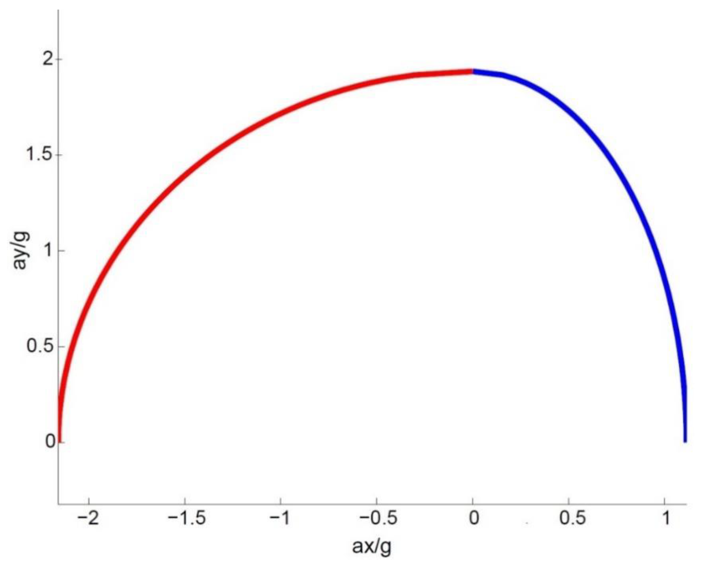
The grip constraint can be studied through the well-known friction ellipse [21]. Given its symmetry in terms of lateral acceleration behaviour, only half of the ellipse will be considered. Mathematically, the locus is determined once the values of the semi-axes are given. Because of the effect of aerodynamics, the size of the ellipse is speed dependent. The longitudinal and vertical aerodynamic forces, $F_x$ and $F_z$, respectively, can be expressed as follows:

$$\begin{gathered} F_x=\frac{1}{2}\rho c_{x}S{v}^2=k_x{v}^2 \\ {F}_z=\frac{1}{2}\rho c_{z}S{v}^2=k_z{v}^2 \end{gathered}$$

(3)

where $\rho$ is the air density, $S$ is the frontal area, and $c_x$ and $c_z$ are the drag and downforce coefficients, respectively. The tyre model herein adopted is based on the assumption that the maximum available tyre–road frictional force is proportional to the vertical load on the tyre, through the friction coefficient $\mu$. Therefore, the ellipse semi-axes can be obtained directly from the dynamic equilibrium equations:

$$\begin{gathered} m{a}_{x+,grip}=\frac{1}{2}\mu mg+\left(\frac{1}{2}\mu k_z-k_x\right)v^2\hspace{1em}acceleration \\ m{a}_{x-,grip}=-\mu mg-\left(\mu k_z+k_x\right)v^2\hspace{1em}braking \\ m{a}_{y,max}=\mu \left(mg+k_z{v}^2\right) \end{gathered}$$

(4)

where $m$ is the vehicle mass, $g$ is the gravitational acceleration, $a_{x+,grip}$ is the maximum achievable longitudinal acceleration when the vehicle accelerates, $a_{x-,grip}$ is the maximum achievable longitudinal acceleration when the vehicle brakes, and $a_{y,max}$ is the maximum achievable lateral acceleration. The last three quantities determine the ellipse semi-axes. In the first equation, the coefficient ½ reflects the assumption that the vehicle is either front-wheel-drive (FWD) or rear-wheel-drive (RWD), as well as the simplified hypotheses that load transfers are neglected and that the downforce effect is evenly distributed between the front and rear axles of the vehicle.

For a generic vehicle condition with the lateral acceleration expressed as $a_y=v^2/R$ ($R$ is the radius of curvature), the achievable longitudinal acceleration according to the grip constraint is as follows:

$$\begin{gathered} a_{x+}=a_{x+,grip}\sqrt{1-{\left(\frac{a_y}{a_{y,max}}\right)}^2}\hspace{1em}acceleration \\ {a}_{x-}=a_{x-,grip}\sqrt{1-{\left(\frac{a_y}{a_{y,max}}\right)}^2}\hspace{1em}braking \end{gathered}$$

(5)

Figure 1 shows an example of the obtained ellipse for $v=50$ km/h.

The constraint on engine power can be expressed as follows:

$$a_{x+,power}=\frac{P-k_x{v}^3}{mv}$$

(6)

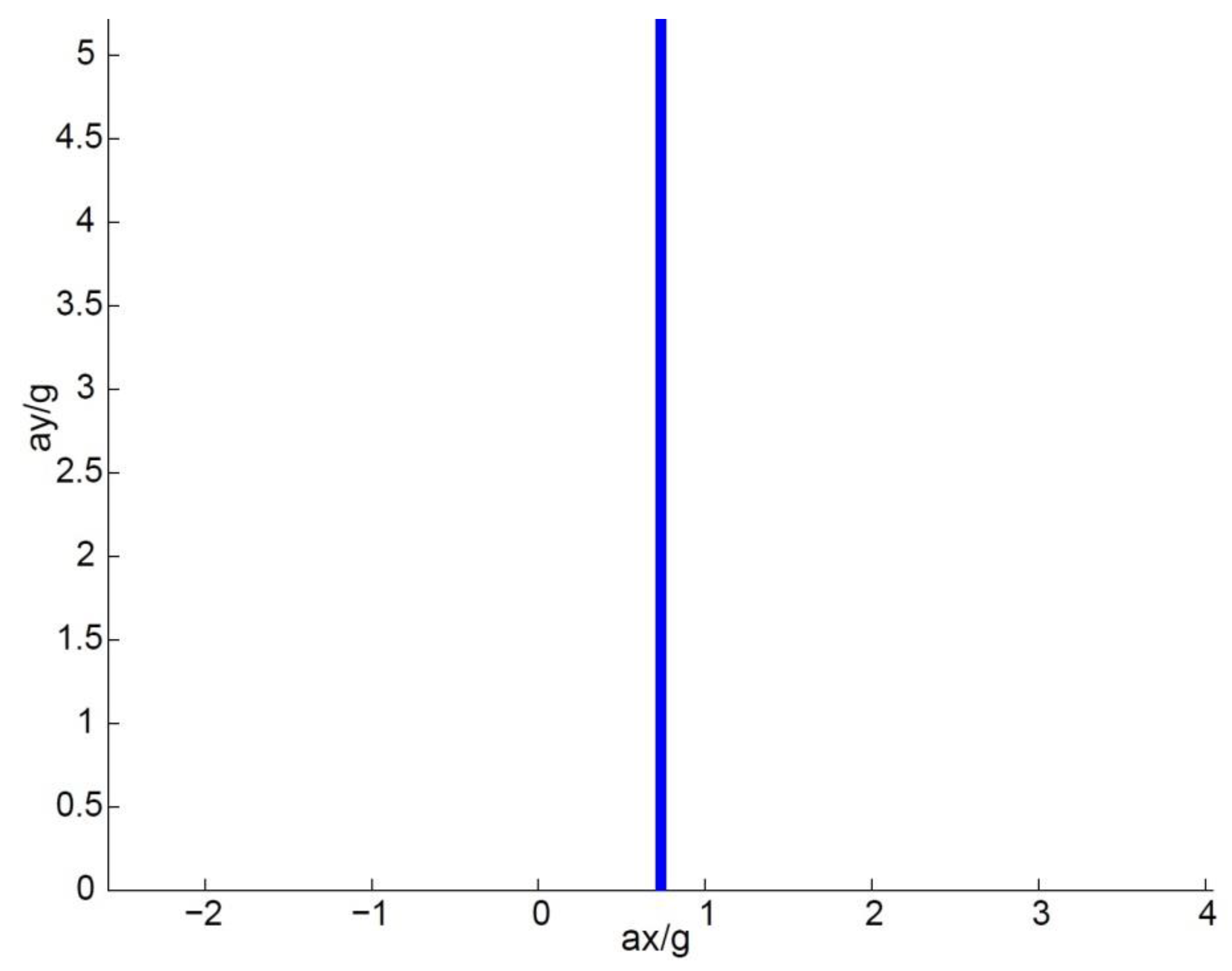
where $P$ is the available power. As shown in Figure 2, the locus is just a vertical line.

The overall vehicle performance bounds are determined by the most restrictive conditions between the grip limit and power limit. In acceleration conditions, the maximum achievable longitudinal acceleration, $a_{x+,max}$, is given by:

$$a_{x+,max}=\min \left(a_{x+},a_{x+,power}\right)$$

(7)

while in braking conditions, the maximum achievable longitudinal acceleration, $a_{x-,max}$, is as follows:

$$a_{x-,max}=a_{x-}$$

(8)

In other words, at each point of the trajectory, $a_y=v^2/R$ is calculated, then Equations (7) and (8) provide the maximum acceleration/deceleration, accounting for the effect of the friction ellipse and maximum power.

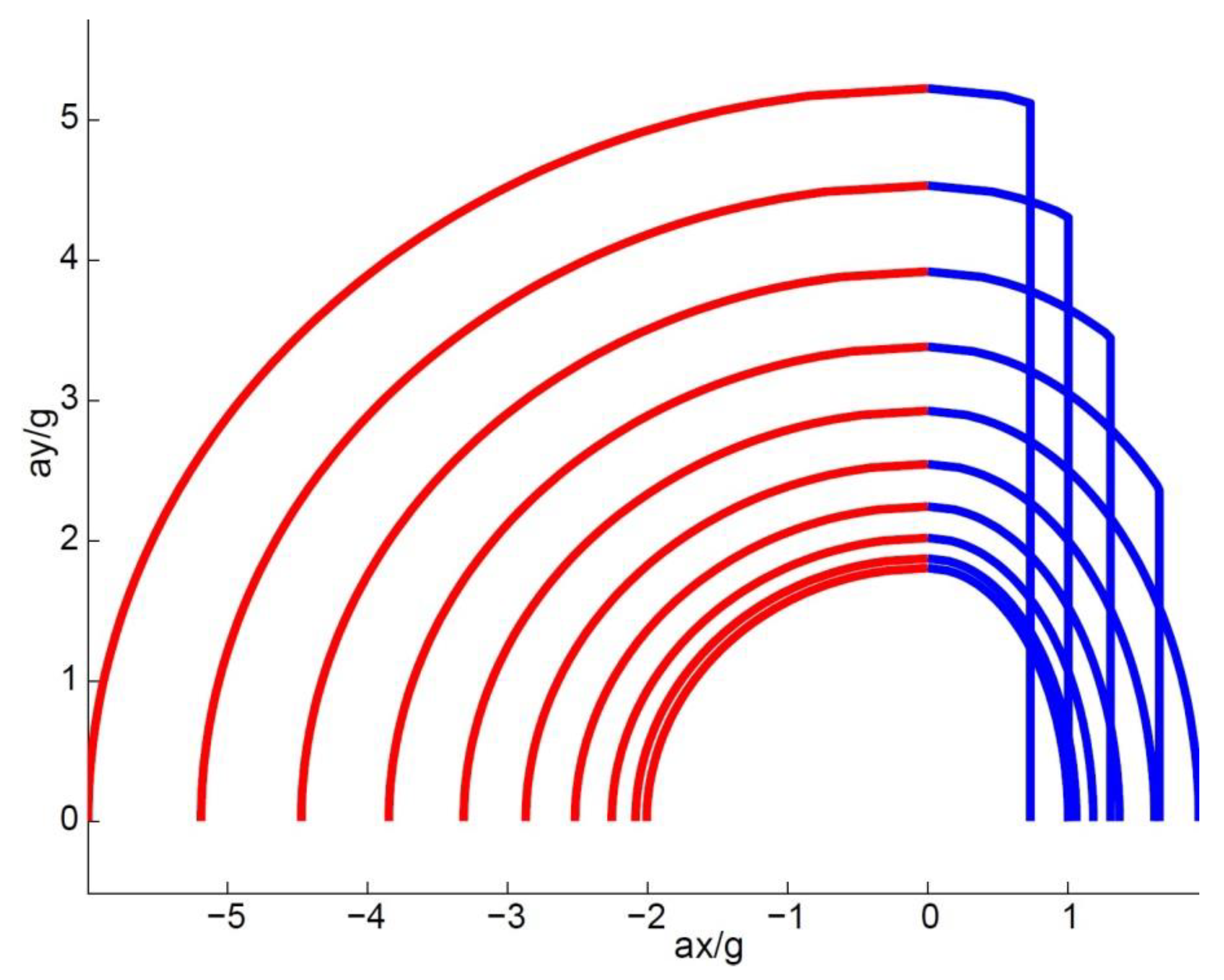
The resulting overall performance bounds are depicted in Figure 3 for speeds from 10 to 250 km/h in 24 km/h steps. Equation (7) inevitably leads to a discontinuity of the derivative at the boundary between the grip and power constraints. There is no discontinuity for low speeds, meaning that the performance is limited by the grip. However, as the speed increases, the discontinuity shows up and the vehicle performance is limited by power. This means that the driver can negotiate the corner at full throttle, without the risk of skidding, as there is high availability of grip.

As stated earlier, the availability of the grip increases with the vehicle speed because of the downforce effect. The vehicle will not skid, as long as the following equation is satisfied:

$$\frac{m{v}^2}{R}\le \mu mg+\mu k_z{v}^2$$

(9)

from which it can be observed that if the radius of the curvature is large enough, there is no grip-related speed limit. The radius of the curvature for which this happens, denoted as the critical radius of the curvature, $R_{crit}$, can be easily worked out as follows:

$$R_{crit}=\frac{m}{\mu k_z}$$

(10)

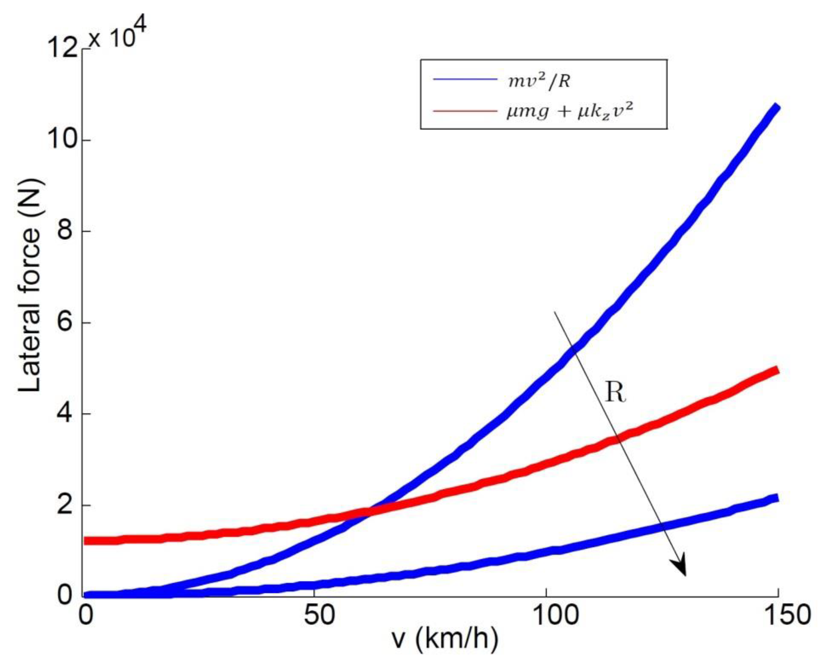
Another way to interpret this is by looking at the left- and right-hand sides of Equation (9)—they are two parabolas, with $v$ as the independent variable. If $R<R_{crit}$, the parabolas have an intersection point, which represents the maximum speed that can be achieved as a result of the grip constraint. If there is no intersection, there is no speed limit. This is seen in Figure 4, which depicts the two parabolas for two values of $R$, one lower and one greater than $R_{crit}$.

3. Optimisation Approach

From the literature, it is known that a generic curve, $\gamma$, can be parameterized with any parameter. Denoting with $t$ (the tangent unit vector) and $k$ (the curvature), in general, the following relationships hold [22]:

$$\mathit{t}=\frac{d\mathit{\gamma }/d\lambda }{\left|d\mathit{\gamma }/d\lambda \right|}=d\mathit{\gamma }/ds$$

(11)

and

$$k=\left|\frac{{\mathrm{d}}^2\mathit{\gamma }\left(s\right)}{\mathrm{d}{s}^2}\right|=\left|\frac{d\mathit{t}}{ds}\right|$$

(12)

where the relationship between the generic parameter, λ, and the arc length, $s$, is as follows:

$$s\left(\lambda \right)={{\displaystyle \int }}_0^{\lambda }\left|\frac{\mathrm{d}\mathit{\gamma }\left(u\right)}{\mathrm{d}u}\right|\mathrm{d}u$$

(13)

which implies $\left|d\mathit{\gamma }/ds\right|=1$, already used in Equation (11).

As the vehicle performance bounds imply that $a_y=\frac{v^2}{R}=k{v}^2$ cannot exceed $a_{y,max}$, there is a maximum allowable speed at each $\lambda$:

$$v_{max}\left(\lambda \right)=\sqrt{\frac{a_{y,max}}{k}}$$

(14)

Such maximum speed plays a key role in the definition of the optimal driver behaviour. Therefore, knowledge of the curvature, $k,$ is crucial.

Practically, curves are often written in terms of a parameter, $\lambda ,$ which is not the arc length. To work out $k$, a potential strategy would be to calculate $s\left(\lambda \right)$ using Equation (13), find $\lambda \left(s\right)$ by inversion, express the curve using the curvilinear abscissa $\gamma \left(\lambda \left(s\right)\right),$ and then calculate $k$ using Equation (12). However, this approach might not be straightforward. For instance, in the simple case of a planar ellipse, $\gamma \left(\lambda \right)=\left(acos\lambda ;bsin\lambda \right)$ can be used as the parameterisation, where $a$ and $b$ are the ellipse semi-axes. The computation of the curvilinear abscissa leads to an integral that cannot be expressed by elementary functions (elliptical integral). As an alternative, Equation (11) can be used in Equation (12):

$$k=\left|\frac{d\mathit{t}}{ds}\right|=\left|\frac{d\mathit{t}}{d\lambda }\frac{d\lambda }{ds}\right|=\frac{1}{\frac{ds}{d\lambda }}\left|\frac{d\mathit{t}}{d\lambda }\right|=\frac{1}{\left|\frac{d\gamma }{d\lambda }\right|}\left|\frac{d\mathit{t}}{d\lambda }\right|$$

(15)

where the second term on the right-hand side can be expanded, using Equation (11), as follows:

$$\left|\frac{d\mathit{t}}{d\lambda }\right|=\left|\frac{d}{d\lambda }\left(\frac{d\mathit{\gamma }/d\lambda }{\left|d\mathit{\gamma }/d\lambda \right|}\right)\right|=\left|\frac{\frac{{\mathrm{d}}^2\mathit{\gamma }}{\mathrm{d}{\lambda }^2}\left|d\mathit{\gamma }/d\lambda \right|-\frac{d}{d\lambda }\left(\left|d\mathit{\gamma }/d\lambda \right|\right)d\mathit{\gamma }/d\lambda }{{\left|d\mathit{\gamma }/d\lambda \right|}^2}\right|$$

(16)

and applying the chain rule, the derivative of the norm of $d\mathit{\gamma }/d\lambda$ can be calculated as:

$$\frac{d}{d\lambda }\left(\left|d\mathit{\gamma }/d\lambda \right|\right)=\frac{d}{d\left(\frac{d\mathit{\gamma }}{d\lambda }\right)}\left(\left|d\mathit{\gamma }/d\lambda \right|\right)\frac{d\left(\frac{d\mathit{\gamma }}{d\lambda }\right)}{d\lambda }=\frac{d}{d\left(\frac{d\mathit{\gamma }}{d\lambda }\right)}\left(\left|d\mathit{\gamma }/d\lambda \right|\right)\frac{d^2\mathit{\gamma }}{d{\lambda }^2}=\frac{{\left(d\mathit{\gamma }/d\lambda \right)}^T}{\left|d\mathit{\gamma }/d\lambda \right|}\frac{d^2\mathit{\gamma }}{d{\lambda }^2}$$

(17)

Replacing Equation (17) into Equation (16), and then into Equation (15), leads to the following:

$$k=\frac{1}{\left|\frac{d\mathit{\gamma }}{d\lambda }\right|}\left|\frac{d\mathit{t}}{d\lambda }\right|=\frac{1}{\left|\frac{d\mathit{\gamma }}{d\lambda }\right|}\left|\frac{\frac{{\mathrm{d}}^2\mathit{\gamma }}{\mathrm{d}{\lambda }^2}\left|d\mathit{\gamma }/d\lambda \right|-\frac{{\left(d\mathit{\gamma }/d\lambda \right)}^T}{\left|d\mathit{\gamma }/d\lambda \right|}\frac{d^2\mathit{\gamma }}{d{\lambda }^2}d\mathit{\gamma }/d\lambda }{{\left|d\mathit{\gamma }/d\lambda \right|}^2}\right|$$

(18)

and finally, is simplified to the following:

$$k=\frac{\left|\frac{{\mathrm{d}}^2\mathit{\gamma }}{\mathrm{d}{\lambda }^2}-\frac{{\left(d\mathit{\gamma }/d\lambda \right)}^T\frac{d^2\mathit{\gamma }}{d{\lambda }^2}}{{\left(d\mathit{\gamma }/d\lambda \right)}^2}d\mathit{\gamma }/d\lambda \right|}{{\left|d\mathit{\gamma }/d\lambda \right|}^2}$$

(19)

which allows for calculating $k$ for a curve expressed with a generic parameter, λ, without using $s$.

To minimise the lap time, at each time step, the driver needs to maximise the vehicle speed as well as the magnitude of the total acceleration. The main challenge for working out the optimal behaviour boils down to figuring out where the driver needs to brake in order to keep the vehicle on the assigned trajectory, i.e., satisfying the performance bounds. Other than that, the driver should always accelerate with full throttle. To ensure the performance bounds are met, the driver should brake early enough so that the vehicle speed at the apex of a corner (the point where $k\left(\lambda \right)$ is the maximum, or the curvature radius is minimum) still satisfies $k\left(\lambda \right)v^2\le a_{y,max}$. If the driver brakes too late, this constraint will not be met, hence the vehicle will not be able to stay on the track. If the driver brakes too early, he/she will be able to stay on the track, but the lap time will not be minimised.

The above idea was implemented through a MATLAB script, according to the following pattern:

• Calculate the state of motion at time step $\mathrm{i}$ (or, at the beginning of a simulation, use the initial conditions).
• Calculate all of the future vehicle states of motion assuming that the driver is braking, until $k\left(\lambda \right)$ has a maximum.
• Check whether the speed satisfies $k\left(\lambda \right)v^2\le a_{y,max}$ at any future time step j.
• If the condition above is always met, it means that the driver can accelerate at step i, and then the state of motion at step i + 1 can be calculated. Otherwise, go back one step and impose that the driver is braking at step i − 1.

The interdependency between the track parameters and vehicle states is embedded in the above steps, as the track curvature influences the maximum speed at which a specific portion of the track can be negotiated. The use of a numerical approach introduces an error that depends on the level of discretisation. On the other hand, the greater the accuracy, the narrower the discretisation and the larger the computational time. A trade-off is to be sought between the performance and computational cost. For the simulations presented in this paper, the curvilinear abscissa was discretised with steps of around 0.1 m, resulting in calculation times of up to a few seconds, always lower than the actual lap times. The step size is in line with suggestions from the literature [13].

4. Results

Simulations were carried out through MATLAB for different tracks, using a high-performance race vehicle. The main vehicle parameters are reported in

Table 1. Main vehicle parameters.

Quantity	Symbol (unit)	Value
Mass	m (kg)	620
Drag factor	$k_x$ (Ns2/m2)	0.72
Downforce factor	$k_z$ (Ns2/m2)	2.15
Power	P (kW)	550

. The tracks investigated were as follows:

• Circumferences (radius of 100 or 200 m)
• Ellipse (semi-axes of 100 and 150 m)
• Straight lines and hairpin bend (two straight lines joined by a 180° constant radius bend, with a radius of 100 m)

In the following plots, the vehicle speed is compared against ${\mathit{v}}_{\mathit{m}\mathit{a}\mathit{x}}$ (from Equation (14)), while the longitudinal and lateral accelerations appear normalised with respect to $\mathit{g}$.

4.1. Circumference

Several simulations were carried out, with and without aerodynamic effects. In the case of aerodynamic effects, a trajectory with a radius greater than the critical one was also studied. The initial speed was intentionally small, so as to better analyse the performance of the developed algorithm.

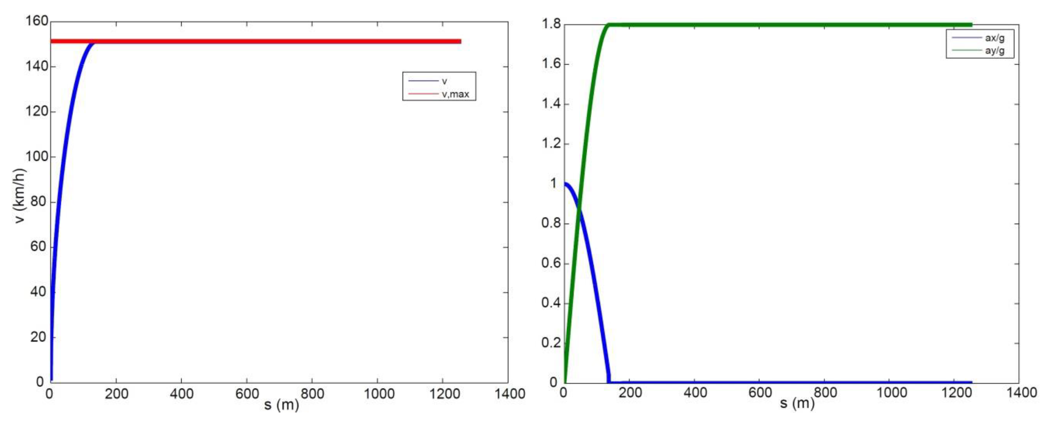
The first simulation was run without aerodynamics effects, and $\mathit{R}=\mathbf{100}$ m. Figure 5 shows speed and accelerations as functions of the arc length. As expected, the vehicle accelerated to reach the maximum speed as soon as possible (Figure 5 (left)). Meanwhile, Figure 5 (right) shows that the lateral acceleration increased at the same time the longitudinal acceleration decreased, because of the effect of the friction ellipse (see Equation (5)). When the maximum speed was reached (around $\mathit{s}\approx \mathbf{150}$ m), Equation (5) shows that the maximum achievable longitudinal acceleration was zero, therefore the vehicle carried on at that speed.

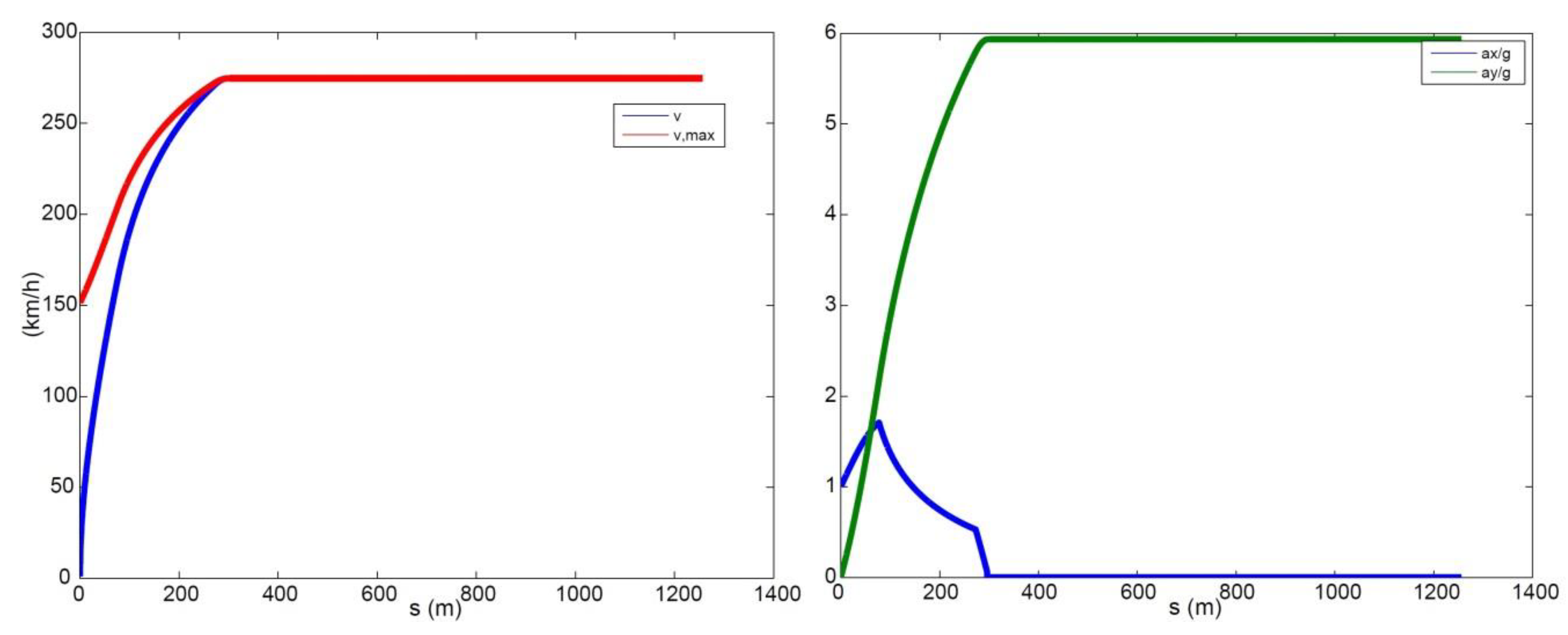
Figure 6 shows the same quantities for a simulation with aerodynamics. The downforce effect clearly increased the maximum achievable speed with respect to the previously analysed case. By looking at the longitudinal acceleration, it increased only until around $\mathit{s}\approx \mathbf{80}$ m, then it was still positive, but decreased as a result of the vehicle power limit.

Using the vehicle parameters from Table 1 in Equation (10), the critical radius was 144 m. Figure 7 shows the results for $\mathit{R}=\mathbf{200}$ m, which is above the critical radius. The maximum speed still increased with the vehicle speed $\mathit{v}$, but was never reached. With $\mathit{R}$ being larger than the critical radius, the maximum velocity will always grow more than the vehicle velocity. However, this time, the maximum velocity was saturated because of the power limit, which intervened rather early (Figure 7 (right)). This implies that, when the negotiated trajectory was approached, there was still a potentially large availability of grip. Theoretically, without a power limit, the speed would keep increasing.

4.2. Ellipse

Two main simulations were carried out, i.e., without and with aerodynamics. Unlike the previous case, the radius of the curvature varied along the path, hence the driver behaviour was not as straightforward as the circumference. Again, the initial speed was relatively small.

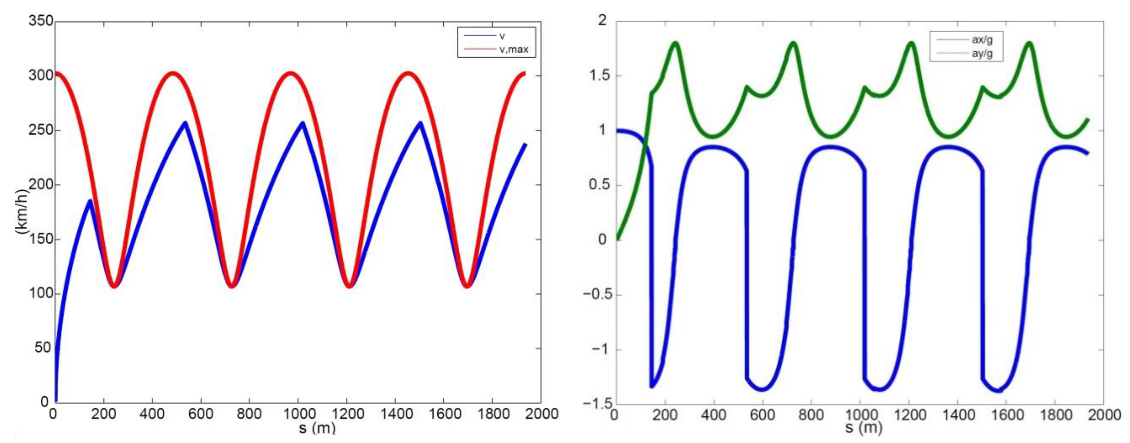
Figure 8 shows the speed and acceleration as functions of the arc length for a simulation without aerodynamics. It is clear that at some point, before reaching the minimum radius of the curvature, the driver needed to brake, so that the speed was equal (without exceeding) to the maximum speed where the curvature was at a maximum (hence the radius of the curvature is at a minimum, which corresponds to the minima of the red curve in Figure 8 (left)).

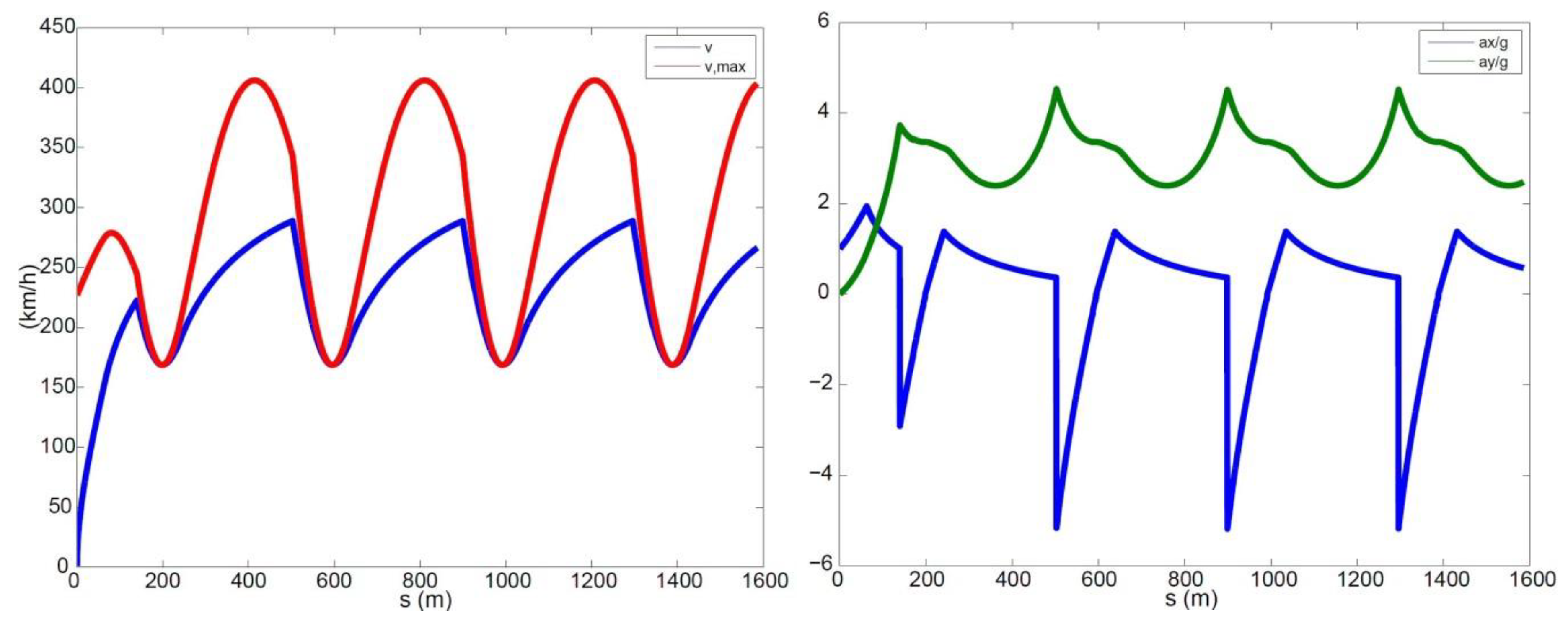
Figure 9 shows the same quantities obtained for a simulation including aerodynamic effects. Again, the maximum speed was increased because of the downforce effect. The vehicle speed increased less sharply than in Figure 8, as the power limits of the vehicle were reached earlier because of the presence of the drag force. On the other hand, the presence of the drag force allowed for a delay in the braking points, which were now much closer to the trajectory apexes (points with minimum radius of curvature).

4.3. Straight Lines and Hairpin Bend

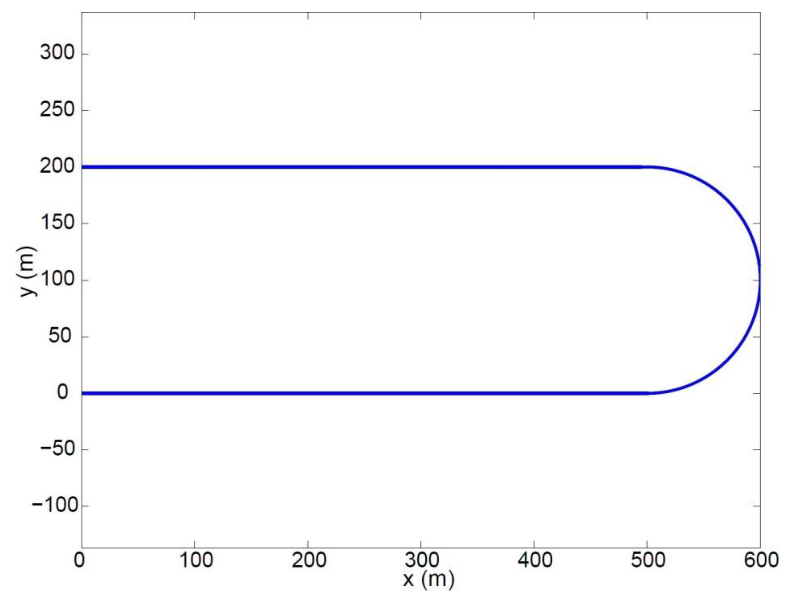
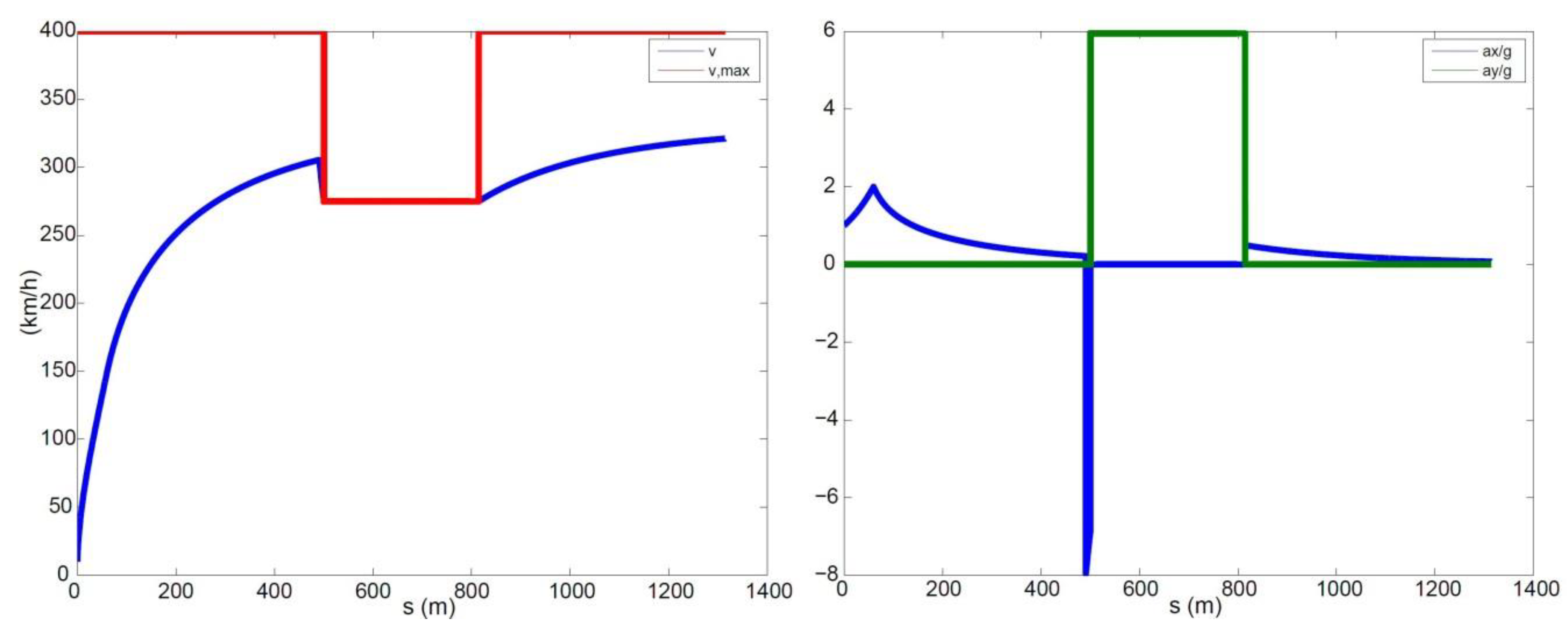
The investigated trajectory consisted of a 500 m straight line, then a constant radius hairpin bend, and finally a straight line identical to the first one (Figure 10). Practically, such a path was obtained by creating a MATLAB script that allowed for the generation of any generic curve starting from its geometric properties, e.g., lengths of the straight lines, bend radii, etc.

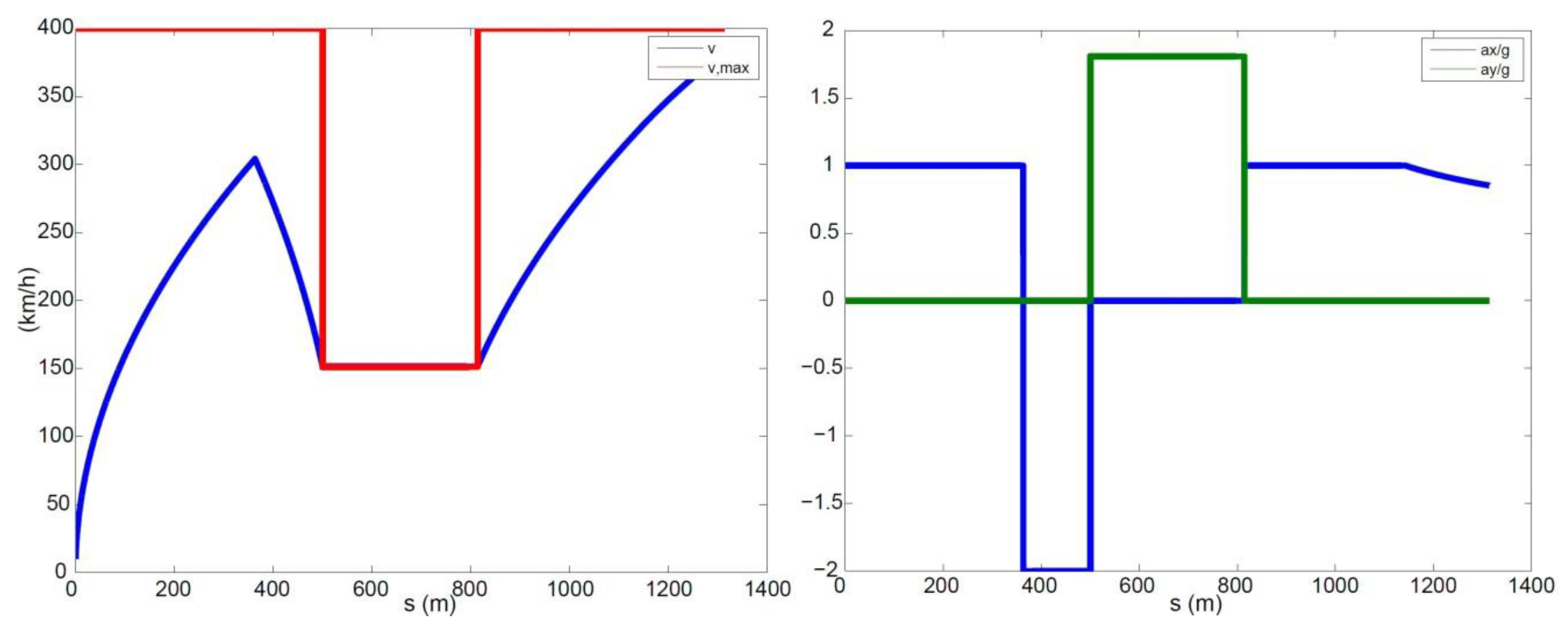
Figure 11 shows speed and acceleration as functions of the arc length for a simulation without aerodynamics. The speed plot shows again that the driver needed to brake rather early in preparation for the bend, which was negotiated at the maximum speed. Once the bend was cleared, the driver accelerated as much as possible. Again, there were important differences when the simulation was carried out including aerodynamic effects (Figure 12). The maximum speed within the bend was obviously higher, which allowed the vehicle to be much faster (around 270 km/h instead of 150 km/h). Interestingly, just before the bend, the achieved speed was around 300 km/h with or without aerodynamics. This was due to the aerodynamic drag, which, on the one hand, triggered the vehicle power limit much earlier, but on the other hand, allowed for braking much closer to the bend.

5. Conclusions

This paper discussed a simple yet insightful method for lap time optimisation. By using a purposely simple vehicle model, the physical constraints as a result of the grip, aerodynamics, and power limit of a generic vehicle were modelled. A rigorous approach was followed in order to work out the curvature of a generic trajectory as a function of a generic parameter which might not correspond to the arc length.

The simulation results allow for the assessment and understanding of the common peculiarities pertaining to the minimum lap time optimisation problem. These include, for example, the combined (longitudinal and lateral) tyre–road interactions, and the effects of both the aerodynamic drag and downforce. Interestingly, the script developed in Section 4.3 will easily allow for the modelling of any real track, which can be well approximated by a mix of straight lines connected through sequences of arcs of circumference.

The computational simplicity of the developed algorithm can be combined with more complicated vehicle/tyre models. As future steps, the authors are working on improving the vehicle dynamics model by: (i) dropping the hypothesis of mass point, (ii) enhancing the tyre modelling, and (iii) extending the algorithm to multi-dimensional tracks. Furthermore, the authors intend to perform appropriate performance comparisons with other methods presented in the literature.

References

1. Metz, D.; Williams, D. Near time-optimal control of racing vehicles. Automatica 1989, 25, 841–857. [Google Scholar] [CrossRef]
2. Van Leeuwen, P.M.; de Groot, S.; Happee, R.; de Winter, J.C. Differences between racing and non-racing drivers: A simulator study using eye-tracking. PLoS ONE 2017, 12, e0186871. [Google Scholar] [CrossRef] [PubMed] [Green Version]
3. Gadola, M.; Vetturi, D.; Cambiaghi, D.; Manzo, L. A Tool for Lap Time Simulation (No. 962529); SAE Technical Paper; SAE International: Warrendale, PA, USA, 1996. [Google Scholar]
4. Scherenberg, H. Mercedes-Benz Racing Design and Cars Experience (No. 580042); SAE Technical Paper; SAE International: Warrendale, PA, USA, 1985. [Google Scholar]
5. Lenzo, B.; Zanchetta, M.; Sorniotti, A.; Gruber, P.; De Nijs, W. Yaw Rate and Sideslip Angle Control through Single Input Single Output Direct Yaw Moment Control. IEEE Trans. Control Syst. Technol. 2020, 1–16. [Google Scholar] [CrossRef] [Green Version]
6. Dal Bianco, N.; Lot, R.; Gadola, M. Minimum time optimal control simulation of a GP2 race car. Proc. Inst. Mech. Eng. Part D J. Automob. Eng. 2018, 232, 1180–1195. [Google Scholar] [CrossRef]
7. Kirches, C.; Sager, S.; Bock, H.G.; Schlöder, J.P. Time-optimal control of automobile test drives with gear shifts. Optim. Control Appl. Methods 2010, 31, 137–153. [Google Scholar] [CrossRef] [Green Version]
8. Kelly, D.P.; Sharp, R.S. Time-optimal control of the race car: A numerical method to emulate the ideal driver. Veh. Syst. Dyn. 2010, 48, 1461–1474. [Google Scholar] [CrossRef]
9. Tavernini, D.; Massaro, M.; Velenis, E.; Katzourakis, D.I.; Lot, R. Minimum time cornering: The effect of road surface and car transmission layout. Veh. Syst. Dyn. 2013, 51, 1533–1547. [Google Scholar] [CrossRef]
10. Biral, F.; Zendri, F.; Bertolazzi, E.; Bosetti, P.; Galvani, M.; Trivellato, F.; Da Lio, M. A web based “virtual racing car championship” to teach vehicle dynamics and multidisciplinary design. In Proceedings of the ASME 2011 International Mechanical Engineering Congress and Exposition, Denver, CO, USA, 11–17 November 2011; American Society of Mechanical Engineers Digital Collection: New York, NY, USA; pp. 391–401. [Google Scholar]
11. Dal Bianco, N.; Bertolazzi, E.; Biral, F.; Massaro, M. Comparison of direct and indirect methods for minimum lap time optimal control problems. Veh. Syst. Dyn. 2019, 57, 665–696. [Google Scholar] [CrossRef]
12. Brayshaw, D.L.; Harrison, M.F. A quasi steady state approach to race car lap simulation in order to understand the effects of racing line and centre of gravity location. Proc. Inst. Mech. Eng. Part D J. Automob. Eng. 2005, 219, 725–739. [Google Scholar] [CrossRef]
13. Veneri, M.; Massaro, M. A free-trajectory quasi-steady-state optimal-control method for minimum lap-time of race vehicles. In The IAVSD International Symposium on Dynamics of Vehicles on Roads and Tracks; Springer: Cham, Switzerland, 2019; pp. 1–22. [Google Scholar]
14. Siegler, B.; Deakin, A.; Crolla, D. Lap Time Simulation: Comparison of Steady State, Quasi-Static and Transient Racing Car Cornering Strategies (No. 2000-01-3563); SAE Technical Paper; SAE International: Warrendale, PA, USA, 2000. [Google Scholar]
15. Völkl, T.; Muehlmeier, M.; Winner, H. Extended steady state lap time simulation for analyzing transient vehicle behavior. SAE Int. J. Passeng. Cars-Mech. Syst. 2013, 6, 283–292. [Google Scholar] [CrossRef]
16. Lot, R.; Biral, F. A curvilinear abscissa approach for the lap time optimization of racing vehicles. IFAC Proc. Vol. 2014, 47, 7559–7565. [Google Scholar] [CrossRef]
17. Kelly, D.P. Lap time simulation with transient vehicle and tyre dynamics. Available online: https://dspace.lib.cranfield.ac.uk/handle/1826/4791 (accessed on 21 January 2020).
18. Casanova, D. On minimum time vehicle manoeuvring: The theoretical optimal lap. Available online: https://dspace.lib.cranfield.ac.uk/handle/1826/1091 (accessed on 21 January 2020).
19. Malcher, S.; Bargende, M.; Grill, M.; Baretzky, U.; Diel, H.; Wohlgemuth, S. Virtual Optimization of Race Engines Through an Extended Quasi Steady State Lap Time Simulation Approach (No. 2018-01-0587); SAE Technical Paper; SAE International: Warrendale, PA, USA, 2018. [Google Scholar]
20. Mühlmeier, M.; Müller, N. Optimisation of the driving line on a race track. AutoTechnology 2003, 3, 68–71. [Google Scholar]
21. Genta, G. Motor Vehicle Dynamics: Modeling and Simulation; World Scientific: Singapore, 1997; Volume 43. [Google Scholar]
22. Curvature and Normal Vectors of a Curve. Available online: https://math.libretexts.org/Bookshelves/Calculus/Supplemental_Modules_(Calculus)/Vector_Calculus/2%3A_Vector-Valued_Functions_and_Motion_in_Space/2.3%3A_Curvature_and_Normal_Vectors_of_a_Curve (accessed on 30 November 2019).
Figure 1. Friction ellipse for v = 50 km/h, grip effect only (blue line: acceleration, red line: braking).
Applsci 10 01498 g001
Figure 2. Power limit for v = 50 km/h.
Applsci 10 01498 g002
Figure 3. Performance bound for different vehicle speeds.
Applsci 10 01498 g003
Figure 4. Maximum achievable speed as a result of the grip and critical radius of the curvature.
Applsci 10 01498 g004
Figure 5. Circumference, no aerodynamics, R = 100 m: (left) speed and (right) accelerations with respect to s .
Applsci 10 01498 g005
Figure 6. Circumference, aerodynamics, R = 100 m: (left) speed and (right) accelerations with respect to s .
Applsci 10 01498 g006
Figure 7. Circumference, aerodynamics, R = 200 m: (left) speed and (right) accelerations with respect to s .
Applsci 10 01498 g007
Figure 8. Ellipse, no aerodynamics: (left) speed and (right) accelerations with respect to s .
Applsci 10 01498 g008
Figure 9. Ellipse, aerodynamics: (left) speed and (right) accelerations with respect to s .
Applsci 10 01498 g009
Figure 10. Straight lines and hairpin bend path.
Applsci 10 01498 g010
Figure 11. Straight lines and hairpin bend, no aerodynamics: (left) speed and (right) accelerations with respect to s .
Applsci 10 01498 g011
Figure 12. Straight lines and hairpin bend, aerodynamics: (left) speed and (right) accelerations with respect to s .
Applsci 10 01498 g012