Roughening in Nonlinear Surface Growth Model

Abstract

The aim of this paper is to examine the coarsening process in the evolution of the surface morphology during molecular beam epitaxy (MBE). A numerical approach for modeling the evolution of surface roughening in film growth by MBE is proposed. The model is based on the nonlinear differential equations by Kuramoto–Sivashinsky (KS) namely, KS and CKS (conserved KS). In particular, we propose a “combined version” of KS and CKS equations, which is solved as a function of a parameter r for the 1 + 1 dimensional case. The computation provides film height as a function of space and time. From this quantity the change of the width of the film over time has numerically been studied as a function of r. The main result of the research is that the surface width is exponentially increasing with increasing time and the change in surface width for smaller r values is significantly greater over longer time interval.

1. Introduction

One of the great challenges of physics and materials science is to understand the growth and surface morphology of the interfaces, both in nature and in technological applications. A recently developed, highly active field of research in statistical physics is dealing with the understanding of surface growth processes [1,2,3,4,5,6,7,8,9]. Researchers are challenged to explore the relationship between the structure and properties of nanostructured materials, and to develop nanoscale structures in a conscious and planned way. The industrial application of coating processes allows thin layers with prescribed properties to be formed on a solid substrate [2]. Different layer-forming techniques are used to produce films, such as ion-beam sputtering (IBS), molecular beam epitaxia (MBE), chemical vacuum deposition (CVD) or physical vacuum deposition (PVD).

The technique of growth surfaces under MBE has received considerable attention for a wide range of technological and industrial applications. This approach provides unique capability to grow crystalline thin films with precise control of thickness, composition and morphology. This enables scientists to build nanostructures as pyramidal or mound-like objects. The evolution of the surface morphology during MBE growth results from a competition between the molecular flux and the relaxation of the surface profile through surface diffusion. The extraordinary richness of pattern forming during MBE is determined by processes which occur locally at the surface.

During the last 30 years, extensive theoretical and experimental research activity has been devoted to this topic. A comprehensive review can be found in [3]. Theoretical models have been proposed which include dynamic scaling [4,5]. Continuous theory [6], stochastic approaches with nucleation and growth [7], and lattice gauge theory [8] have improved significantly the knowledge of the growth process phenomenon.

In surface dynamic evolution, both surface coarseness and smoothening mechanisms are observed, for example, in MBE and PVD [10,11,12]. During the MBE, a weak particle board is directed to the sample so that the thin layer can be applied in virtually atomic layers and the composition can be easily controlled. In the case of vacuum spray, the particles exert a non-thermal effect on the source but generate plasma. During the two processes, the deposition of the particles and the smoothing of the resulting surface patterns are determined by surface diffusion [9,10,11,12,13,14,15]. On the growing surface, self-similar structures can be observed, but the growth of periodic patterns is unstable. In fact, the growth processes of amorphous thin films can be interpreted in an attractive system. Amorphous structures exhibit isotropic spatiality in the absence of a long-term structural sequence. Experimental studies of amorphous thin films, generated by electron beam atomization, show the formation of mound-like structures in mesoscopic length [2,3,4,5,6,7,8,9,16,17]. Stochastic growth equations of continuous continuum models indicate the complexity of atomic size growth processes [1].

Thin films deposited by vacuum techniques such as MBE typically produce thin film of a thickness in the range of 10–25 μm. In the working chamber of the MBE equipment, each element is steamed separately in steady state. The speed of vaporization of each element and thus the composition of the layer to be created can be controlled very precisely ([10,18,19,20,21]). The MBE method has been developed to produce single-crystal layers of semiconductors. The media is usually kept at a few hundred °C. Atoms arriving on the surface (data meshes) first bind weakly to the surface, migrate and ultimately make a perfect two-dimensional array. Growth speed is relatively slow, usually one monolayer/s.

The benefits of the molecular beam epitaxia are that:

• The parameters can be checked very accurately (the substrate temperature, growth rate, a crystalline layer of orientation),
• The formation of the sheet is continuously monitored,
• It is also applicable for making hetero structured semiconductors with sharp transitions and magnetic thin films,
• It is suitable for mass production.

Several non-independent height sensitive parameters are specified for the analysis of the surface profiles. The measure of the surface morphology are roughness parameters of individual layers and location in the profile. The average surface roughness and surface height are widely used in the industrial practice to characterize the topography of mechanical surfaces. The results of the surface profile and the roughness on friction were studied in [22,23,24,25,26,27,28,29,30,31,32,33,34].

In non-equilibrium physical problems, nonlinear dynamics and pattern formation have attracted the attention of researchers to physical, chemical and biological processes for several decades. It has become clear that similar phenomena play a key role in nanostructured processes. While in case of macro and microsystems it is a great advantage to control the processes with special tools and devices, for nanoscale these devices are missing, or their use is prohibitively expensive [10]. This indicates that the observation of the pattern formation and spontaneous self-organization is particularly promising in controlling of these methods. Structural coatings with nanostructured thin films can generate or control the pattern of the deposition. The size and shape of nanostructures are spontaneously generated by the internal stress or using external stress.

Our goal is to understand and to predict their temporal evolution of thin films. The aim of this paper is to develop numerical simulations to the physical model to obtain surface structure depending on time and parameters involved in the physical model and to determine the temporal change of the width of the film in some special cases.

2. Physical Background

In the mathematical approach, it is very important to incorporate the uncertainties of the parameters into the model. The main sources of uncertainties are difficult to predict. These are for example, the atomic level of elastic conjoint effects and surface state changes. Partial differential equations describing the characterization of irregular surfaces are provided with free boundary conditions. Partial differential equations cannot be solved analytically or only very rarely, and the numerical algorithms used are generally unstable. Therefore, variational methods are required. Governing equations describing the phenomenon are usually strongly nonlinear differential equations.

In the surface coating processes, the initial state of the substrate is an almost flat surface, the particles in the vapor are perpendicular to the surface and the deposition process is characterized by the deposition flux. Particles on the surface go through various surface diffusion processes when they reach their final position. The growing surface layer is composed of these particles after a certain time. The height or morphology $H\left(\mathrm{t},\mathrm{x},\mathrm{y}\right)$ of the surface layer depends on time $t$ and spatial coordinates $x,y$. The evaluation of the surface structure is determined by the particles arriving on the surface and by the condensed particles on the surface. The process in time and space is determined by the interplay of different mechanisms such as coarseness, smoothening and shape formation. To examine the roughness of the surface, we control the height profile with $h\left(\mathrm{t},\mathrm{x},\mathrm{y}\right)=H\left(\mathrm{t},\mathrm{x},\mathrm{y}\right)-Ft$, where $F$ is the mean deposition rate and $h$ satisfies the equation:

$$h_t=G\left(\nabla h\right)$$

with a functional $G$ of spatial derivatives and depending on the setting parameters of the deposition procedure and material parameters.

Our goal is to investigate deterministic equation whose solutions are properly characterizing the physical phenomenon and from which the results obtained with the initial condition are likely to remain valid even after a long period of time. The equations are sometimes supplemented with stochastic members that represent temperature or instrumental noises. In this paper we do not address the effects of noise.

The processes in time $t$ are analysed in one dimension by one spatial coordinate $x$. The surface height is characterized by the height function $h\left(t,x\right)$ from the theoretical plane surface.

For amorphous growth processes temporal and translational invariance in growth direction and in the direction orthogonal to growth are considered [3]. The isotropy of the amorphous phase implies invariance under rotation and reflection around the direction of growth. Therefore, the presence of the derivatives terms of odd order of $h\left(t,x\right)$ is not allowed. The symmetry up and down ($h\to -h$) is necessary. The dynamics can be described by effective one-dimensional equations.

The simplest equation describing the film growth is the Edward–Wilkinson model [18]:

$$h_t=\nu h_{xx}+\eta ,$$

(1)

where the indices denote the derivative with respect to the variable $t$ or $x$, and $\nu$ is constant and $\eta$ denotes the noise term. The term $\nu h_{xx}$ is the surface tension.

For example, when desorption is important, the growth can be described by the Kardar–Parisi–Zhang equation [4] which is considered as the paradigm of the stochastic roughening. For the analytical treatment of the vapor phase deposition of thin films, a nonlinear term was added to Equation (1) to model the deposition and formation of a thin film:

$$h_t=\nu h_{xx}+\lambda {\left(h_x\right)}^2+\eta ,$$

(2)

where $\lambda$ is a constant. In Equation (2), $h_t$ represents the rate of absorption, the first term at the left side the relaxation of the interface and the second term the tendency of the surface locally growing normal to itself.

Specially, the Kuramoto–Sivashinsky (KS) equation is a paradigm of the deterministic dynamic system which leads to the complex spatial and temporal chaotic behavior of the physical phenomenon with applications in flame fronts, plasma ion waves and chemical phase turbulence [19]. Its general form is of the form:

$$h_t=-h_{xx}-h_{xxxx}+{\left(h_x\right)}^2,$$

(3)

where $h_{xxxx}$ takes into account the diffusion. Equation (3) was originally derived in the context of plasma instabilities, flame front propagation and phase turbulence in reaction-diffusion system [9].

In case of vanishing desorption and weak asymmetry, a modified form of Equation (3) is used to model amorphous thin film layers and roughening processes of the surface, where the nonlinear member is replaced by a nonlinear member on the right:

$$h_t=-h_{xx}-h_{xxxx}-r {\left(h_x\right)}_{xx}^2.$$

(4)

Equation (4) is the so-called ‘conserved Kuramoto–Sivashinsky’ (CKS) equation [35,36], where parameter $r$ is a parameter.

In our investigations a combined version of the (KS) and (CKS) equations will be analyzed

$$h_t=-h_{xx}-h_{xxxx}+{\left(h_x\right)}^2-r {\left(h_x\right)}_{xx}^2,$$

(5)

where the third term at the right side equilibrates the slope dependent adatom concentration. Equation (5) considers relaxation mechanisms, lateral growth, surface diffusion, and desorption and is suitable to characterize the coarsening of thin films. Benlahsen et al. [11] gave an analytic solution in closed form and it was used for examining the coarsening. Munoz-Garcia, Cuerno and Castro [12] have derived and analyzed numerically the growth model (5).

3. Numerical Results

In this paper, the solution to (5) is examined with numerical simulations. These results help us to explain the phenomena observed by experiments and validate the mathematical model. So, we follow the stress effects in understanding the physical phenomena. Our choice for the initial condition applied to (5) which mimics the initial surface structure of the substrate:

$$h\left(0,x\right)=1cos\frac{x}{16}\left(1+sin\frac{x}{16}\right)$$

(6)

The solution of the one-dimensional combined CKS Equation (5) subjected to (6) is determined numerically by using Fourier spectral collocation in space and the fourth order Runge-Kutta exponential time differencing scheme for time discretization. Numerical solution for height profiles are calculated for different values of $r$ with the following data:

$$x\in \left[0,32\pi \right], t\in \left[0,250\right],N=256,\Delta t=1/100.$$

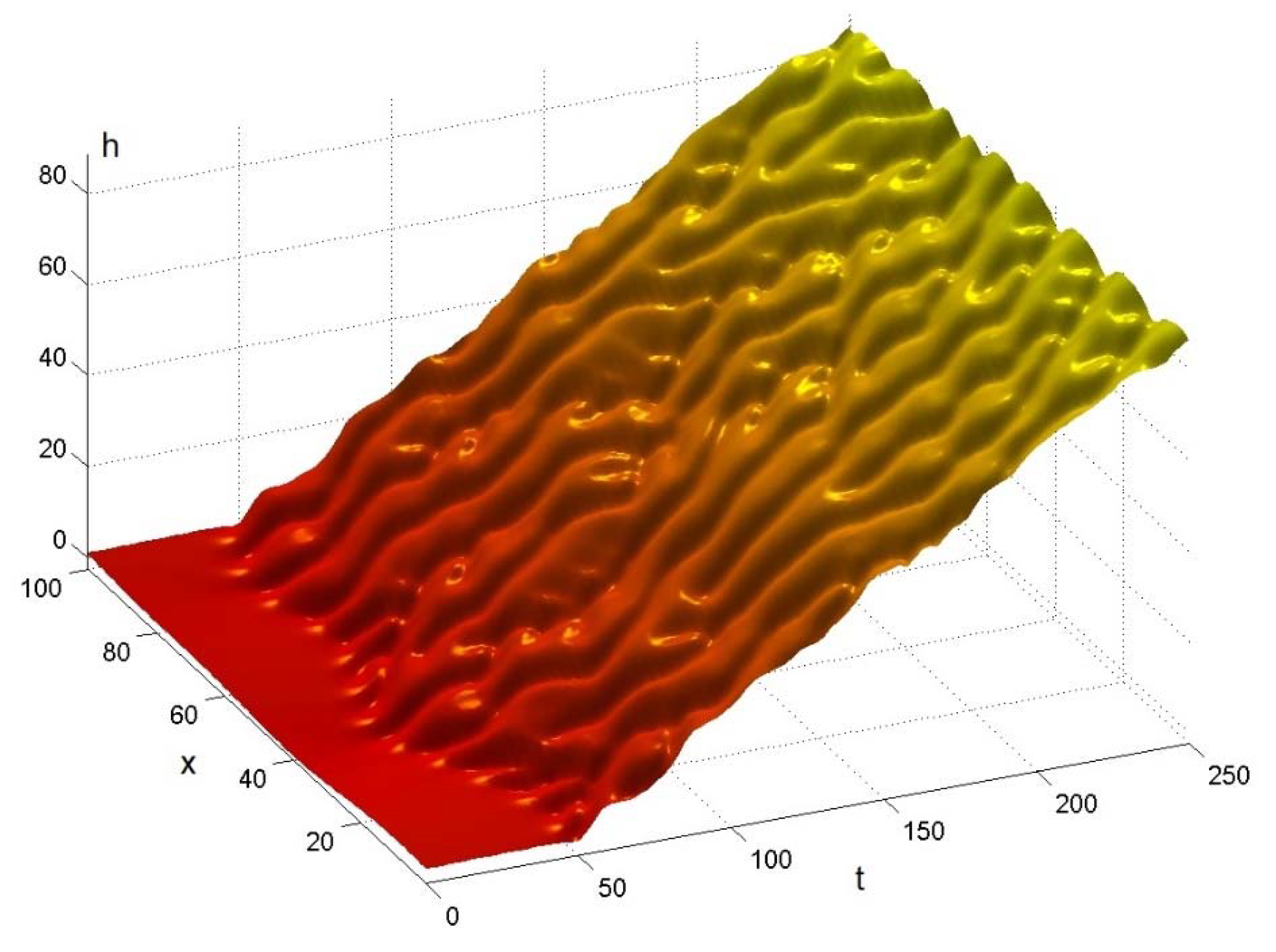
The surface height profile $h\left(t,x\right)$ is shown on Figure 1 calculated from the nonlinear deterministic growth Equation (5) in 1+1 dimension using the parameter $r=0.01$. We can observe that the evaluation of $h$ starts about $t=$50 for initial condition (6). We note that for taking an amplitude greater than $A=1$ in (6), the evaluation of $h$ starts earlier. In Figure 1 we see the chaotic evaluation of the ripples which merge and split at different t and x. 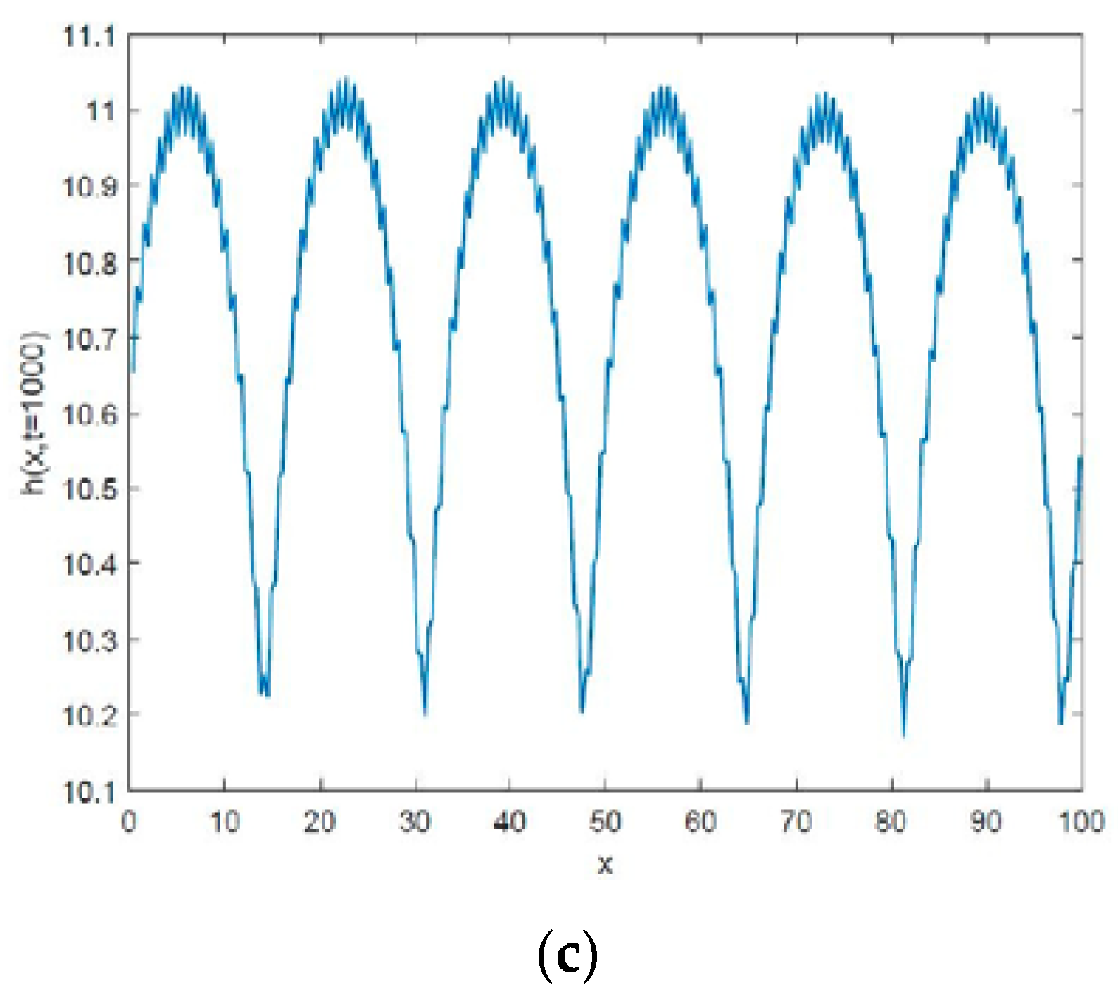Figure 2 illustrates the cross-section of the surface structure at fixed time $t=1000$ for different values of $r$ ($r=0.01, 0.5, 1$.) It can be seen that with increasing $r$ the cross section became more regular. For large $r \left(r=1\right)$, the cross section at $t=1000$ shows periodicity like $\left|\sin x\right|$.

The temporal evaluation of the film roughness described by its height profile $h\left(t,x\right)$ can be seen in Figure 2. The surface roughness is characterized by the surface width $w\left(t\right)$ which is defined by the rms fluctuation in the $h\left(t,x\right)$, in time $t$ for a linear size $L$ of the sample.

Statistical evaluation of the parameters is calculated on the surface (mean, standard deviation, etc.). On the profile, where data points are joined by line segments the linear interpolation is applied, but a spline interpolation provides usually closer result to the continuous profile. The texture parameters are calculated, the approximation method by summations is replaced by integrals. To ensure the correctness, the parameter definitions are given for the continuous functions, i.e., parameters are expressed with integrals.

In modern specification standards, parameter definitions are always given for the continuous case, i.e., expressed with integrals. In case of statistical evaluation of the parameters for the microgeometry of the surface, it is convenient to centre the height function in the evaluation of the surface texture parameter, i.e., the mean height is subtracted from the height. The use of continuous definitions ensures the correctness of the definition and does not imply any numerical approximation.

In this paper, the change of roughness in time is illustrated by the function $w\left(t\right)$ with the deviation from the average height as follows:

$$w^2\left(t\right)=\frac{1}{L}{{\displaystyle \int }}_0^L{\left[h\left(x,t\right)-\overline{h}\left(t\right)\right]}^{2}dx$$

(7)

where the average height function $\overline{h}\left(t\right)$ is calculated with the form:

$$\overline{h}\left(t\right)=\frac{1}{L}{\int }_0^{L}h\left(x,t\right)dx.$$

Function $w\left(t\right)$ is used to call the mean interface width. We recall that in our calculations $L=32\pi$.

4. Roughening

One of the most important tasks in tribology is to design surfaces tailored to operation. Tribological parameters are important in studies and many of them show strong correlation with surface operational performance. The surface texture affects the contact and temperature conditions between the contacting surfaces. These conditions define the tribological process and the wear mechanism occurring between the surfaces.

We note that in papers [11,12] analytical and numerical results were given to Equation (5). In both cases $r=50$ is considered. In [11] a truncated parabola was chosen as the initial condition. In [23], the initial height values were uniformly chosen between 0 and 1 randomly. In comparison the solutions show the same structure in $h$ an in $w$ for large t ($t=1000$) in [12] for $r=50$ and in our case for $r=10$; the parabolic or $\left|\sin \right|$ solutions show periodicity and they have the same amplitude. The authors noted that there are parabolic cells grow in width and height in time and the coarsening process slows down until stopping completely. In [11] it was shown that the amplitude behaves as $0.5lnt$ for large values of $t$.

Several evaluation techniques are known to test surface microgeometry [37,38]. In industrial practice, the parameter-based characterization is used to provide general roughness (Ra). There is a long list of parameters employed in the industry and the standard [39,40] defines the method and parameters of evaluation. The field parameters use the data point measured in the area examined. Applying field parameters, the surface heights, the slopes and the wavelength can be evaluated.

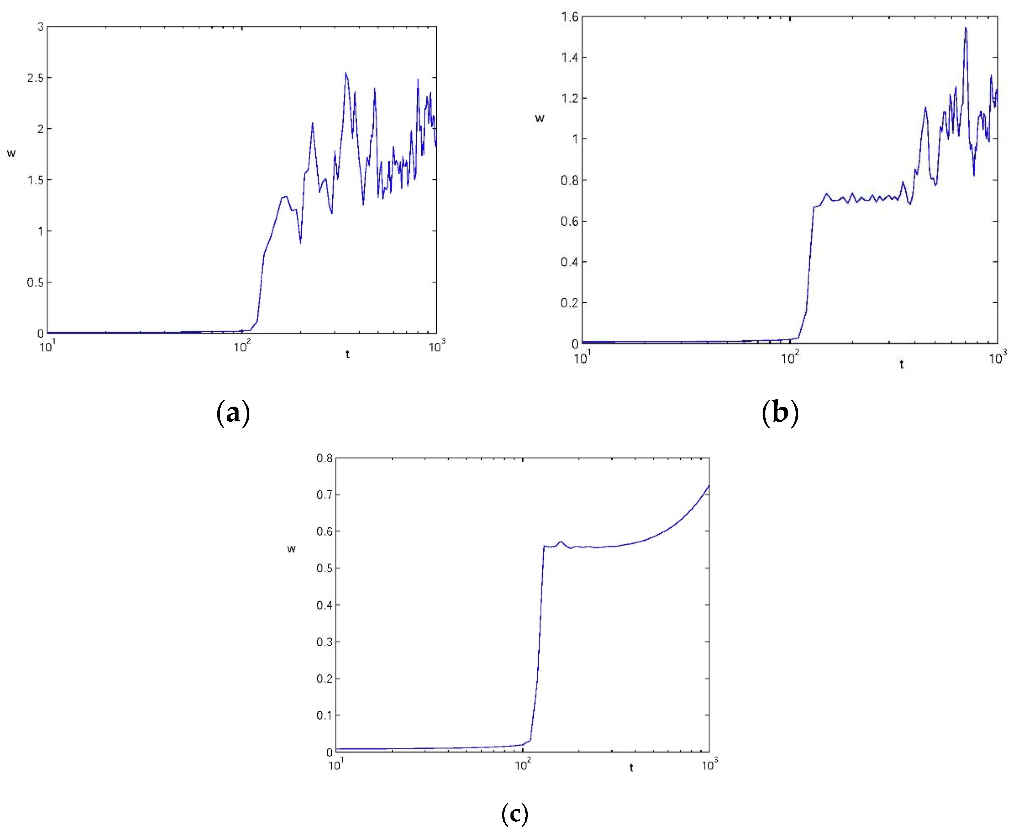
Figure 3 introduces the surface width calculated from the solutions (5)–(6) with formula (7). It can be seen from Figure 3 that the surface roughening only starts after approximately 50 time units. This time depends on the quality of the initial surface. Our simulations show that when in the boundary condition (6) and the amplitude of 1 on the right side of the equality decreases to 0.01, $h\left(0,x\right)=0.01cos\frac{x}{16}\left(1+sin\frac{x}{16}\right)$, this surface roughening starts at approx. 120 time units. It can be stated that the smoother the starting surface the later the coarsening of the surface topography appears. The shape of the curves is also influenced by the coefficient $r$, which combines the material and physical parameters in Equation (5). We can conclude that $w\left(t\right)$ is smoother for higher values of $r.$

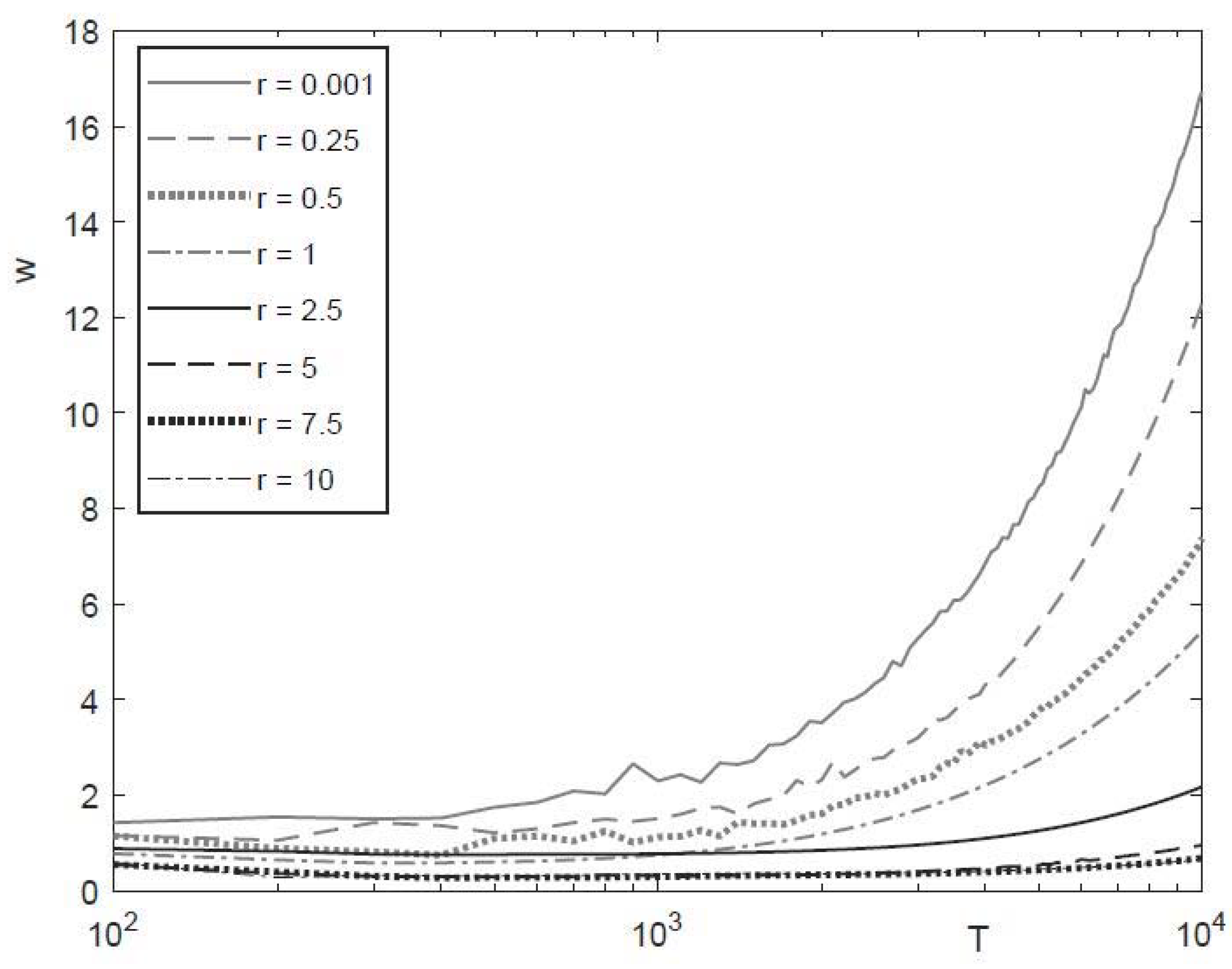
The time dependence of the surface width is exhibited on Figure 4 for different values of $r$. We can also see that, for the given time, the surface roughness is decreases with increasing parameter $r$. Moreover, for large $t$, the surface width $w$ is exponentially increasing with time $t.$

5. Conclusions

Although several growth models have been introduced in the literature, the understanding of growth processes is very important. We address the problem of MBE growth in one spatial direction. The time-dependent growth equation introduced by the combined Kuramoto–Sivashinsky equation is investigated using the model (5).

In this paper we concentrate on the surface evolution and the surface roughening. We performed simulations for the surface profile applying various values of the parameter $r$. The profile is strictly depending on the initial condition (on the profile of the substrate at the beginning) and on the value of the parameter $r$ involved in Equation (6). If $r$ is small, i.e., the impact of the term ${\left(h_x\right)}_{xx}^2$ is small, chaotic ripple formation appear. The surface morphology is characterized by the surface width $w\left(t\right)$.

The roughening starts at approximately 50 time units. The evolution of surface morphology is affected by parameter $r$. Figure 2, Figure 3 and Figure 4 demonstrate the effect of parameter $r$. The surface width is exponentially increasing with increasing time and it is decreasing with increasing parameter value $r.$

We performed simulations for our growth model for simplicity in 1 + 1 dimensions, but it can be straightforwardly generalized to any dimension.