Simplifying the Verification of Simulation Models through Petri Net to FlexSim Mapping

Abstract

Simplifying the encoding of a simulation conceptual model representation reduces the number of errors that will be detected in the verification phase. In this paper, we present a mapping between Petri nets, a well-known formalism, and FlexSim, a well-known simulation tool. The proposal is illustrated through an example of how a model specified in a Petri net can be encoded easily, reducing the time needed to understand and verify the model. In the proposed methodology, the mapping must be defined at the initial stage of the encoding, starting from (in this case) a Petri net conceptual model, and ending at the encoding tool (FlexSim in this case). The main advantages of the proposed methodology are discussed.

1. Introduction

The development of any simulation project is guided by the verification, validation and accreditation processes. The three phases must be carried out in agreement with the hypotheses that govern the model, which are mainly defined in the conceptual model.

The conceptual model to be used to represent the systems must be selected in agreement with the client and experts in the system. In order to simplify the subsequent validation, the experts must focus on the conceptual model and not on any specific encoding, so they must feel confident with the language used to produce conceptual representations of their system. The only requirements for these languages are that they must be complete and unambiguous, and able to define the structure and the behavior of all the model elements, all of which are met by languages like the Specification and Description Language (SDL) [1,2], Petri nets [3,4,5] and Discrete Event System Specification (DEVS) [6] Interestingly once there has been a formal definition of a simulation model one can undertake transformations of the model from one of these formal representations to another; as an example, taking DEVS as a common formalism [7], one can transform an SDL model to DEVS [8] or Petri nets to DEVS [9]. The possibility of transforming the conceptual model from one representation to another allows it to be independent of the final language used to represent this conceptual model. The structure and behavior of the model are preserved.

In this paper we show a mapping between timed Petri nets and FlexSim, proposing a methodology that will simplify the verification and encoding process. This methodology opens the door to the implementation of automatic encoding algorithms for different tools. The mapping can also be extended to colored timed Petri nets since the concept of color is equivalent to the concept of an attribute in the FlexSim target simulation environment. However, it has been decided to narrow the scope of this article mostly to timed Petri nets to facilitate the description of the methodological process.

Figure 1 shows the simplified modeling process [10]; in red are the aspects that will be simplified with the application of the proposed methodology.

2. Literature Review

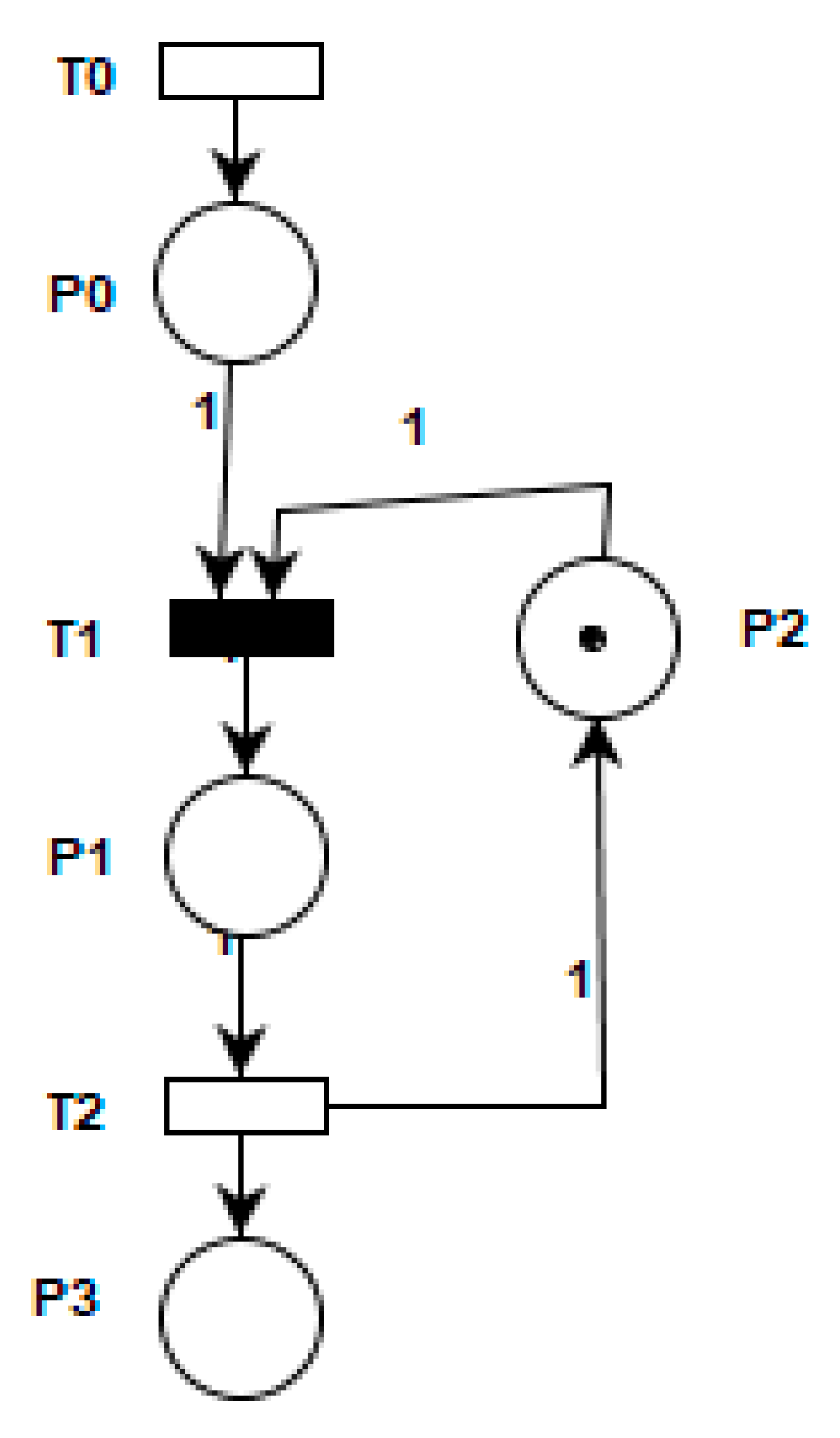
The need for a formal representation to include the stakeholders in the model validation and verification is becoming increasingly relevant because of the growing complexity of the models [11], the use of languages to simplify the communication between the parts to accelerate the agreement is encouraged. For example, in the frame of health, [12] discusses how to assure the engagement of the stakeholders in the modelling process, proposing the use of diagrams and drawings to ensure that the model is fully understood and that an agreement on the parts exists. On the same scope, some solutions are proposed aligned with the idea of representing graphically the model, like on [13,14] where the use of Business Process Model and Notation (BPMN) is proposed, see [15], extending it in order to make it fully executable and unambiguous. Along the same lines, [16] proposed the use of SDL; in that case, due to the nature of the language, SDL is complete and not ambiguous, and one can define the model involving the stakeholders without the need of add an extension to the language. This codification in SDL can be achieved automatically if one uses a tool that understands any of these formal languages, like [17,18,19], among many others. Petri Nets, like SDL does not need the addition of any extension, hence a model defined in a Petri Net is complete and can be fully codified. Petri Nets become an excellent alternative to represent simulation models and to analyze the correctness of executing a task or representing its behavior, in multiple areas, like in robotics and microcontrollers [20,21], to study biological and social systems [22,23,24] or infrastructures and logistics analysis [25,26,27] among other multiple scopes, hence several works exist to transform to Petri Nets models represented in other languages, like BPMN or Flowcharts, see [28,29,30] as an example.

In the frame of Petri nets there exists a database that, although not exhaustive, collects the most important software capable of running a model represented with a Petri Net, see [31]. Some studies have been undertaken to generate cose automatically, from this formalization of the models [32,33,34], but few analyses have been undertaken regarding how to map a conceptual model to one of the more popular all-purpose simulation tools [35] so that through this mapping these generic simulation tools can be used and to take advantage of the features that for a specific project may be needed, without losing the independence of the model with respect to the tool used for the codification. Some applications that combines the use of Petri Nets and FlexSim environment exist, like [36,37], with a mapping in the context of Arena environment [38] and Petri Nets [39], but no description on how to undertake mapping between Petri Nets and the FlexSim environment is detailed. Doing so gives the modelers a clearer picture of how the final tool will encode the different assumptions. Moreover, it guides the encoding process which is simplified and highly automatized.

3. Petri Nets

Petri nets have become established as a powerful modeling formalism in computer science, system engineering, and many other disciplines. They combine well-defined mathematical theory with a graphical representation of dynamic system behavior. The theoretical component provides a precise model of the system behavior for analysis while the graphical component simplifies the visualization of complex systems and enables the representation of changes in the system. This combination is the main reason for the huge spread of the use of Petri Nets [40].

3.1. Basic Definition

A Petri net, see Figure 2, is a specific type of graph comprising three kinds of objects: places, represented by circles; transitions, represented by bars, and directed arcs, which connect places and transitions. The dynamic nature of the system is represented by the movement of entities, in a Petri net, and this can be represented as tokens (drawn as dots) that are dynamically created and destroyed through the net.

A Petri net is formally defined as a 5-tuple N = (P, T, A, W, M₀), where:

• P = {P₁, P₂, P₃, ....., P_np} is a finite set of places;
• T = {T₁, T₂, T₃, ....., T_ne} is a finite set of transitions;
• A = {A₁, A₂, A₃, ....., A_na} is a finite set of arcs that connect places to transitions and vice versa;
• W: A_i → {1, 2, 3, ....} ∀ A_i is the weight associated with each arc;
• M₀: P_i → {1, 2, 3, ....} ∀ P_i is the initial number of entities in each place (initial marking).

The current location and distribution of entities in a Petri net is called a marking.

A transition can be fired if each transition input has the required number of entities specified by the weight associated with the arc from the place to the transition. Firing the transitions (that represent the simulation events) removes entities from the input places and adds entities to the output places. The number of entities removed or added equals the weight of the associated arc [3].

3.2. Timed Petri Nets

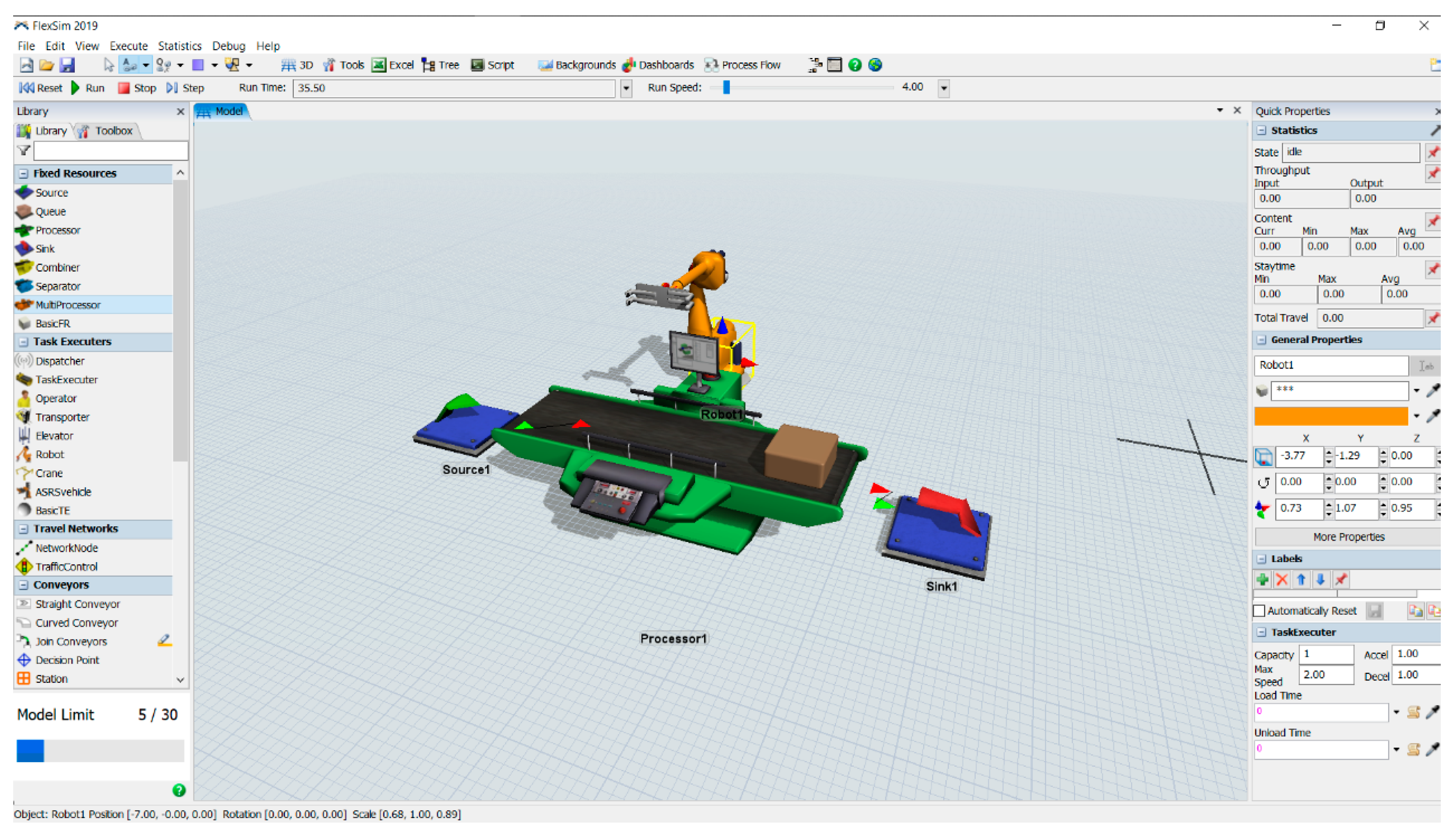
Time is a crucial aspect when dealing with dynamic logistics, manufacturing or transportation processes, such as automatic guided vehicle (AGV) systems. Therefore, the notion of time must be included in the Petri nets. The most commonly used model shows the associated delay time for enabling a transition to be fired.

The firing of a transition in a Petri net corresponds to an event that changes the state of the system. This may be the result of the verification of a logical condition in the system, as discussed in the previous section (immediate transitions) or induced by the completion of an activity, which naturally takes a certain amount of time (timed transitions); see Figure 3.

As a convention, this document will use the PIPE software representation [41,42]: black rectangles for immediate transitions and white rectangles for timed transitions. The white rectangle must have a time function (tf), which specifies the duration of the transition [3].

4. FlexSim

FlexSim^® [43] is a commercial simulation package that allows the execution of discrete and continuous simulation models. Being a commercial suite, it allows the definition of the simulation models following a proprietary and graphical approach, based on the connection of different simulation objects that allows representing the model behavior in a process interaction paradigm [44], see Figure 4.

Like several simulation packages, one of the main features of the tool is the simplification of the model definition and the faster execution of the simulation models. Some interesting features of FlexSim is the capability to generate C++ code from the models and the integration with the internet of things (IoT) through some well-known protocols, like OPC-UA [45]; the OPC (Open Platform Communications) is a set of standards and specifications for industrial telecommunication released in 1996; the UA stands for Unified Architecture (UA), released in 2008, which expands OPC to become a platform-independent service-oriented architecture. OPC-UA integrates all the functionality of the individual OPC classic specifications into one extensible framework.

The use of proprietary tools to define and codify the model implies that the model recodification in other tools (because a requirement in the project changes or because of the end of the live cycle of the product) becomes a complex and time-consuming task. Also, it increases the possibility of errors due to this recodification process.

In order to avoid these drawbacks but without avoiding the use of tools like FlexSim, we propose to define an automatic mapping between a well-known formalism widely used in the simulation frame, timed Petri nets, to FlexSim. Also, FlexSim, allowing the definition of new logics and element templates, can include easily the proposed mapping, allowing an automatic execution of models based on timed Petri net formalism.

5. Mapping Petri Nets to a FlexSim Model

Once a Petri net conceptual model has been created and validated by the problem owners, it is important to determine the validity of the model and its relevance to the executable model. This is achieved using the mapping approaches explained below and finally confirmed in the verification phase.

This state-space and causal or flow process logic expressed in the Petri net must be mapped into a model that uses the FlexSim library blocks. It is convenient to use a table to map the Petri net process model and the transition specifications to a FlexSim model [46]. The Petri net models can then be mapped into the equivalent FlexSim model code.

5.1. Sequential Execution

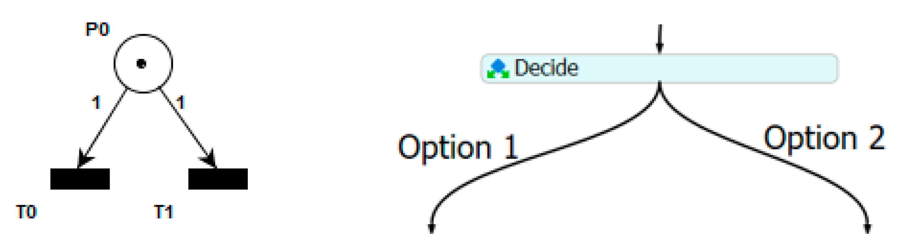
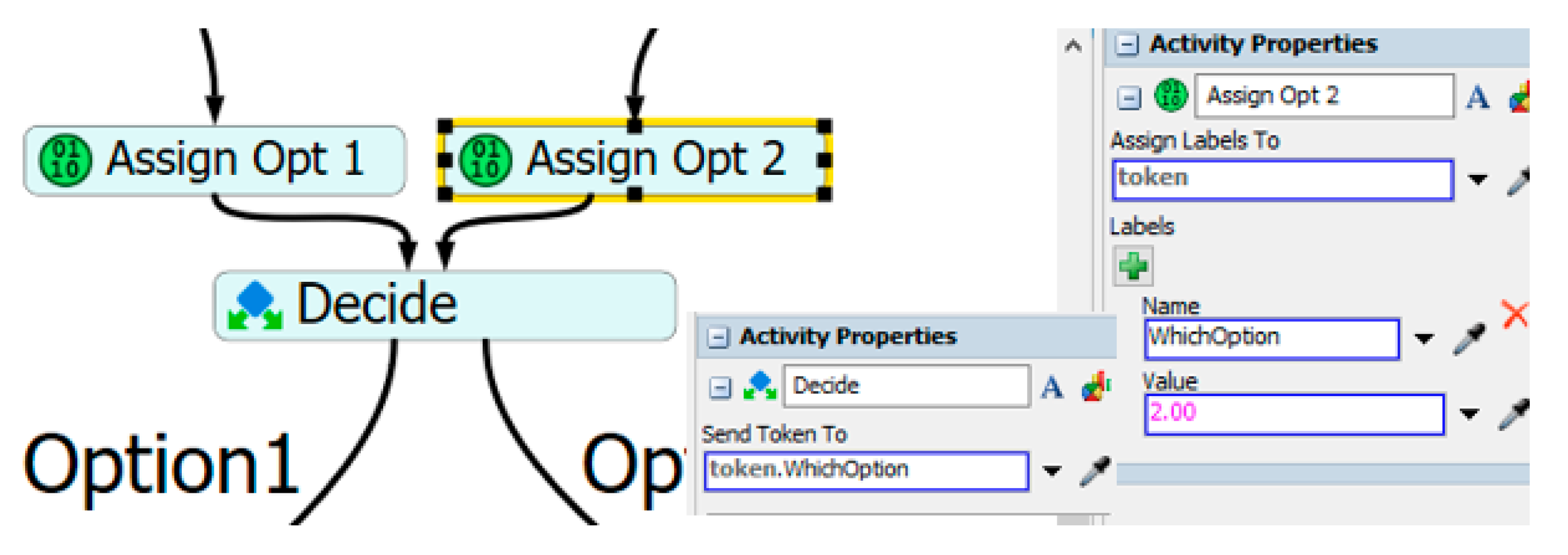
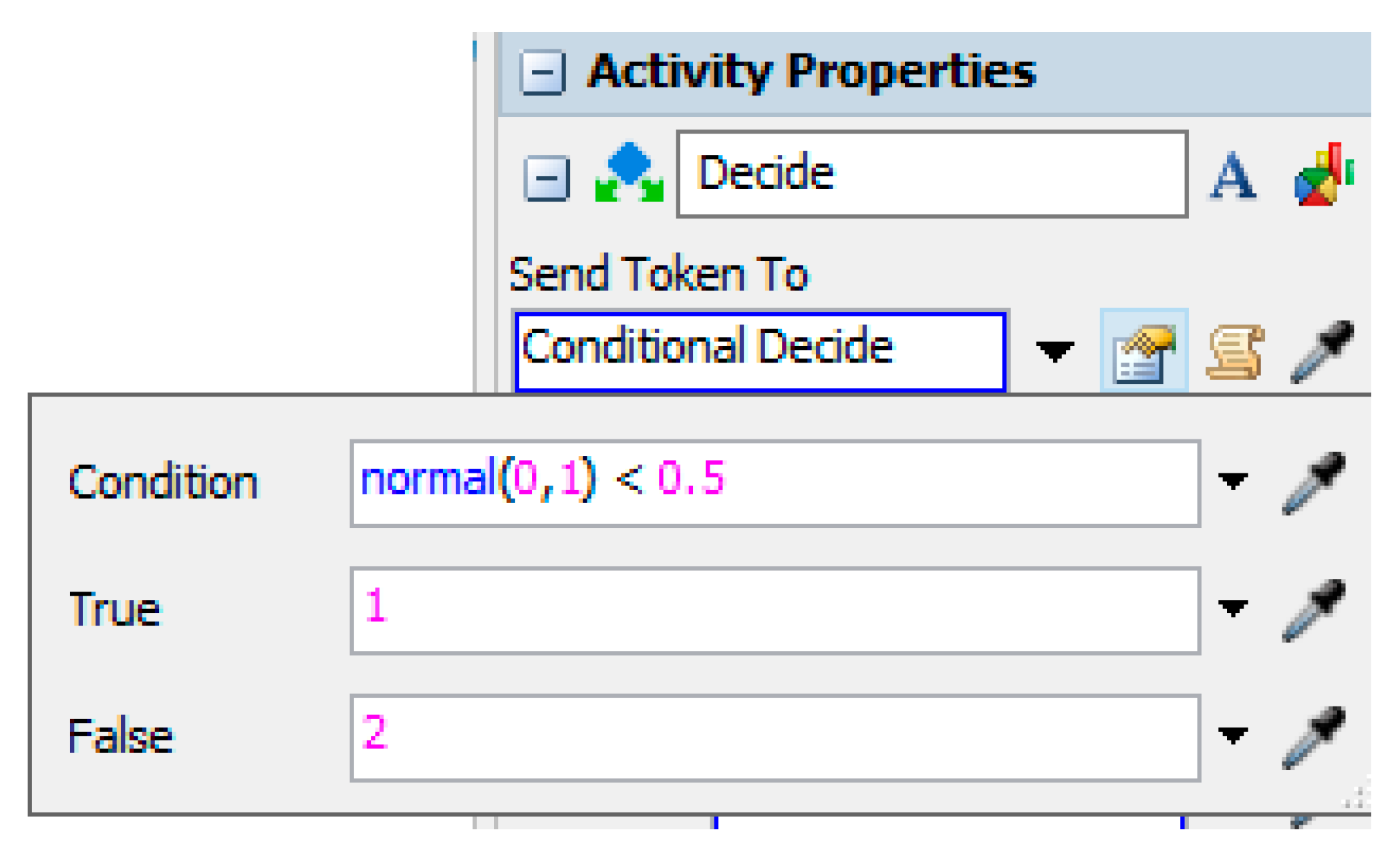
In the Petri net shown in Figure 5, transition T1 can only be fired after T0 has fired. This construct a sequential relationship between activities. The place/timed transition pair can be coded in FlexSim using the Delay activity.

5.2. Conflict

Transitions T0 and T1 are in conflict in this Petri net: both are enabled, but the firing of either one disables the other, see Figure 6. This situation will arise, for example, when an AGV must choose at an intersection between two different routes. The resulting conflict may be resolved in a non-deterministic or probabilistic way. This situation, in which the entity must choose between two different transitions, can be coded in FlexSim using the Decide activity and can also be solved in either of the two ways.

The Decide activity can have one or multiple inputs as well as one or multiple outputs, see Figure 7. Each output is assigned a positive integer number (the first option is 1, the second option is 2, etc.) All inputs enter the Decide activity and exit to the assigned output. Therefore, the deterministic or probabilistic solution of the conflict will depend on the number that is “assigned” to each token, as the number assigned for each output is not changeable. For a deterministic solution, labels (equivalent to colors in a colored Petri net) can be used. These labels can be assigned before the Decide activity or may exist from previous processes.

Let us imagine that, depending on the weight of the cargo, we will choose one option or another (deterministic decision). Specifically, if the cargo weighs less than 1000 u, it will exit by option 1; otherwise, it will exit by option 2. This can be configured in FlexSim by assigning the labels previously, see Figure 8.

Conflict can also be solved probabilistically using this system, but in this case, a statistical expression must be added. For instance, in Figure 9 the condition is selected by a normal distribution. There are several different statistical distributions, such as Bernoulli, Uniform, Poisson, etc.

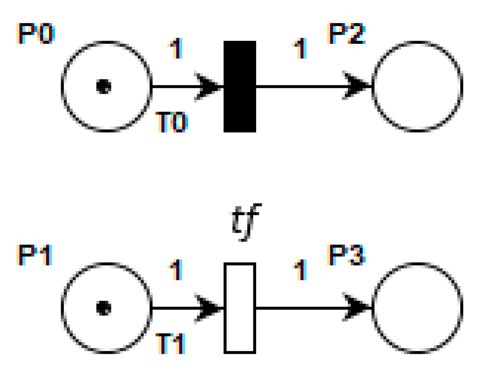
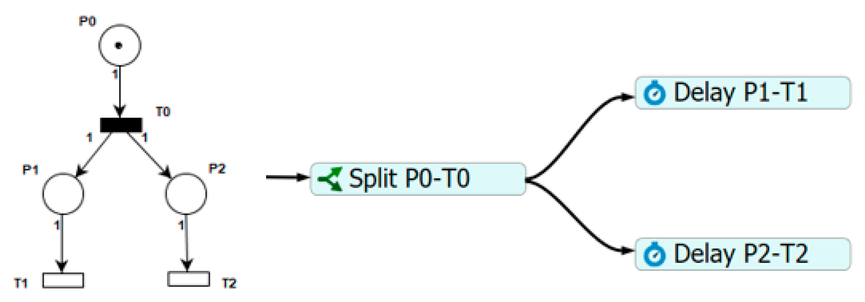
5.3. Concurrency with Temporal Entities

In Figure 10, T1 and T2 transitions are concurrent. Concurrency is an important attribute of system interactions. In order to create concurrent transitions, there must be a forking transition that deposits a temporal entity at two or more output places. This might represent, for example, an AGV that transports two packages and splits the cargo indiscriminately between two conveyor belts. The Split activity in FlexSim deposits temporal entities at two (or more) output places.

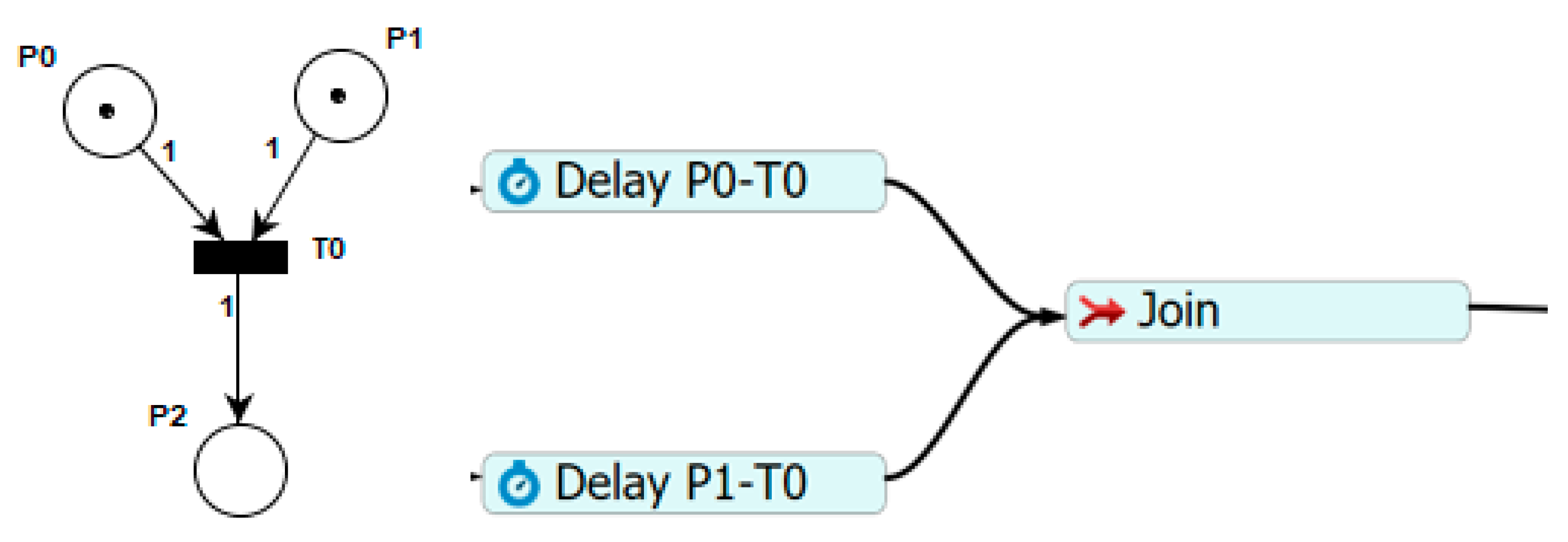
5.4. Synchronization with Temporal Entities

In Figure 11, places P0 and P1 need to receive an entity in order for T0 to be enabled. Synchronization is common in a dynamic system for an event to occur. This can be represented, for example, by a situation in which two pieces need to be assembled before being transported. The existence of two different parts makes no sense at the point at which they are joined to form a single entity.

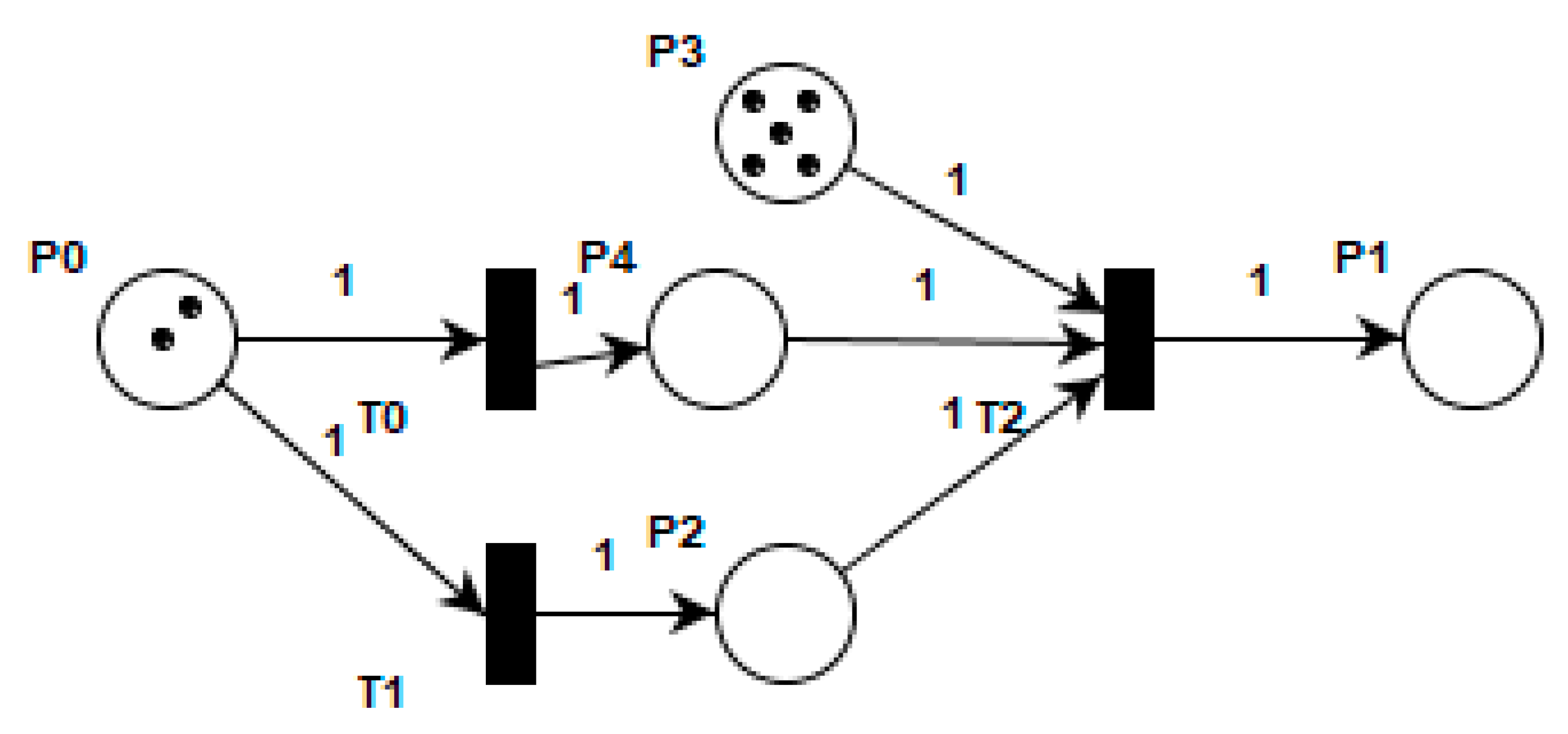
5.5. Concurrency and Synchronization with Resources

The timed Petri net shown in Figure 12 models a single-queue single-server process. This is a classic queuing model in which arriving entities (T0) wait in a queue (P0) for the resource. When the resource becomes available (P2) it starts to process the entity (if there is an entity in P0), remaining at P1 (working) until T2 is fired. The resource returns to P2 and final pieces go to P3. As can be seen, the model provides resource synchronization (P0-P2-T1) and concurrency (T2-P2-P3).

This whole Petri net can be simulated using Join and Split activities, as explained above. However, because resources are so common in Petri nets, and in order to provide a rapid and comprehensive view of the scheme (imagine using the same resource for several concurrent Petri nets), they have specific activities. Therefore, Figure 12 can be represented in FlexSim as shown in Figure 13.

This simple scheme is the basis for resource use in our manufacturing systems. For example, it might signify the use of an AGV (the resource), and the delay is the product transportation time from the source to the destination.

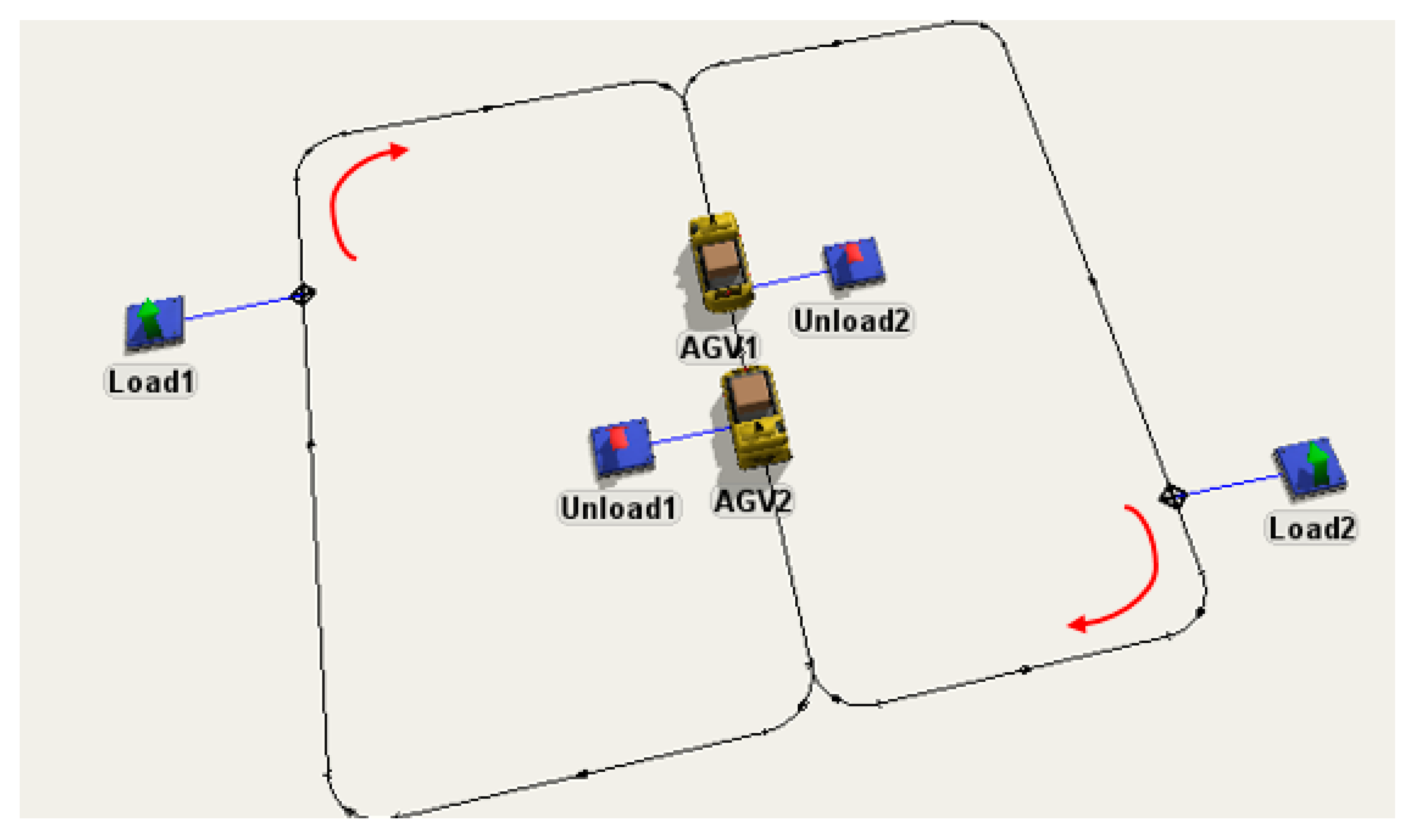
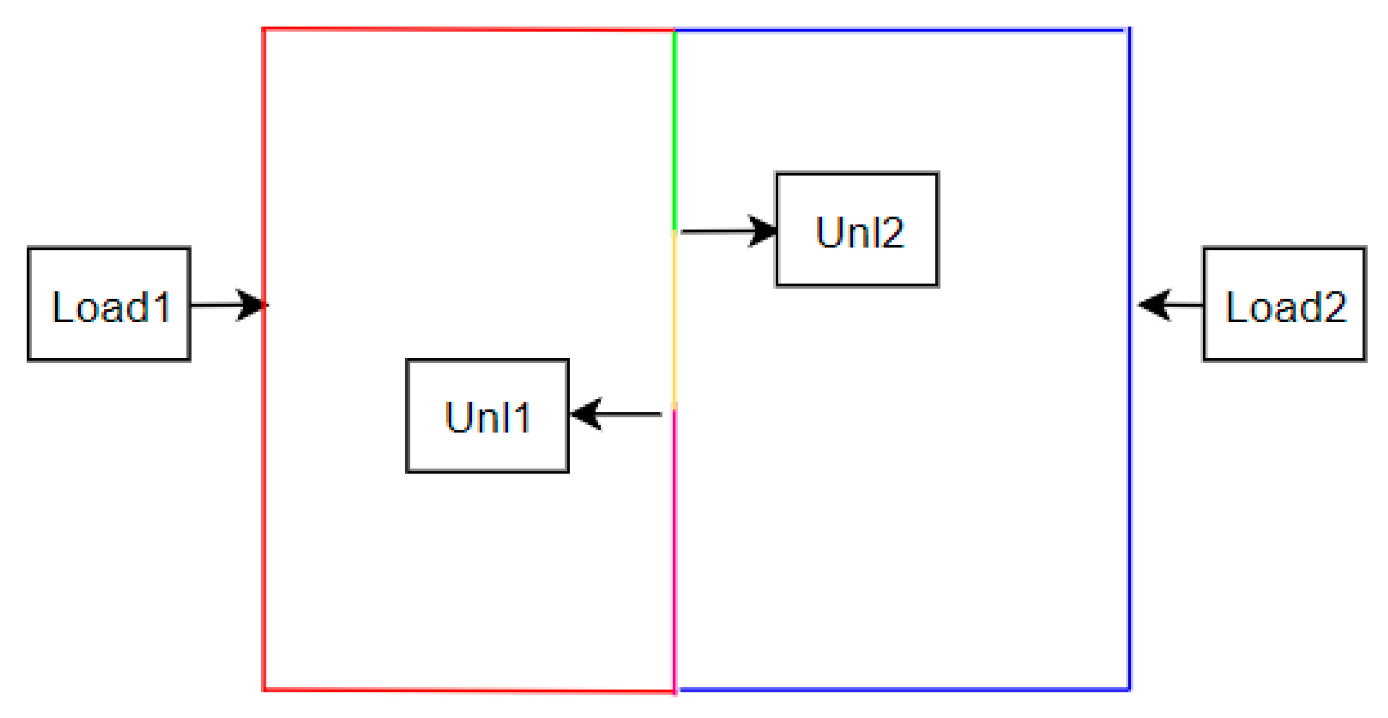
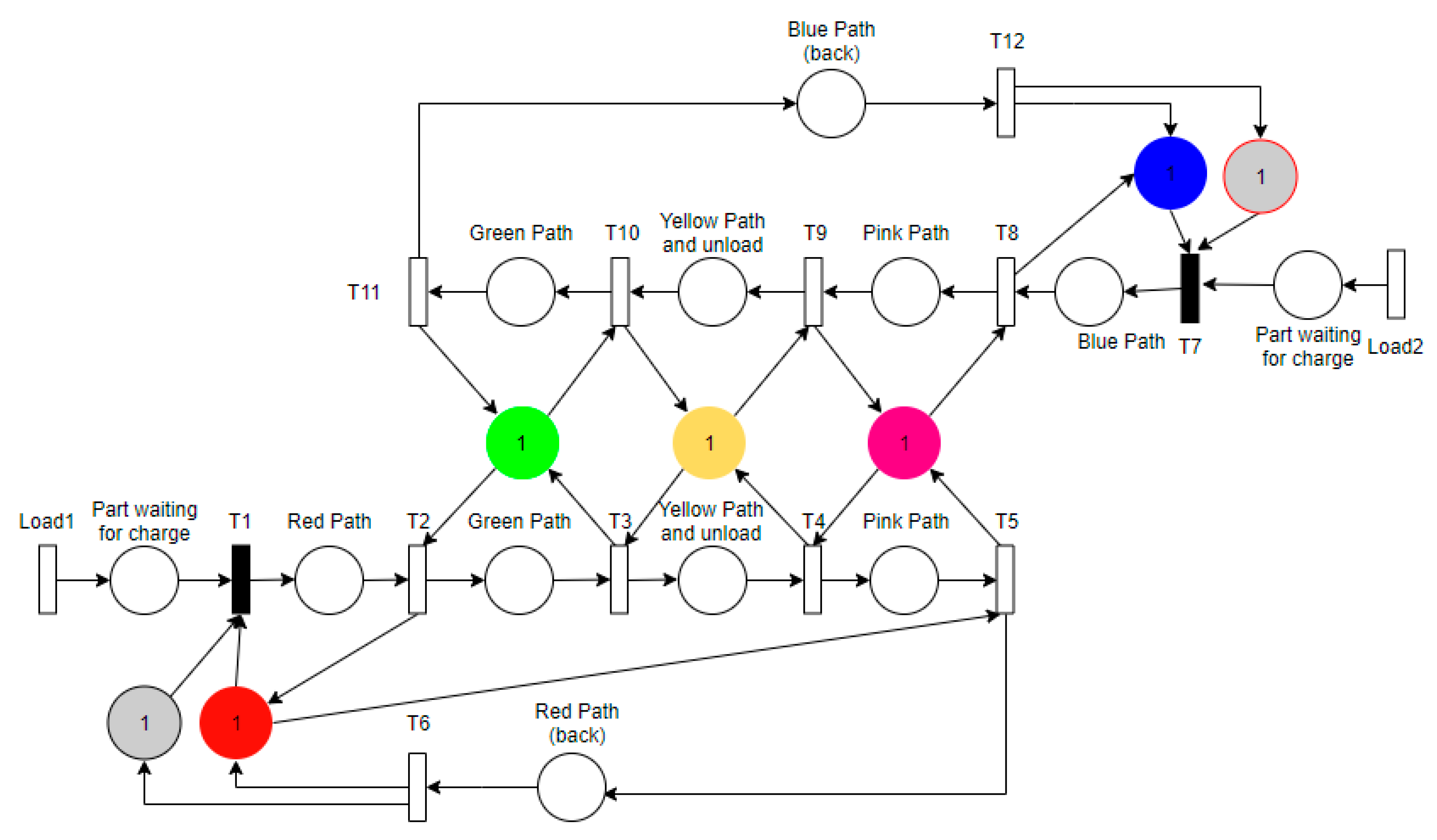
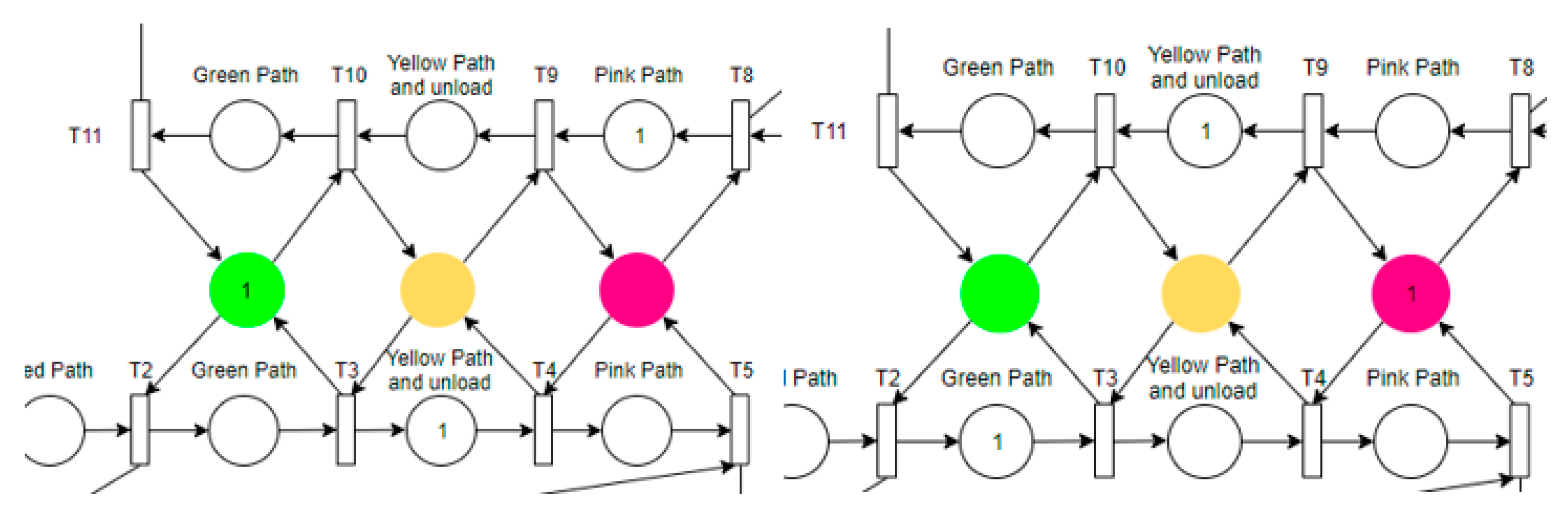
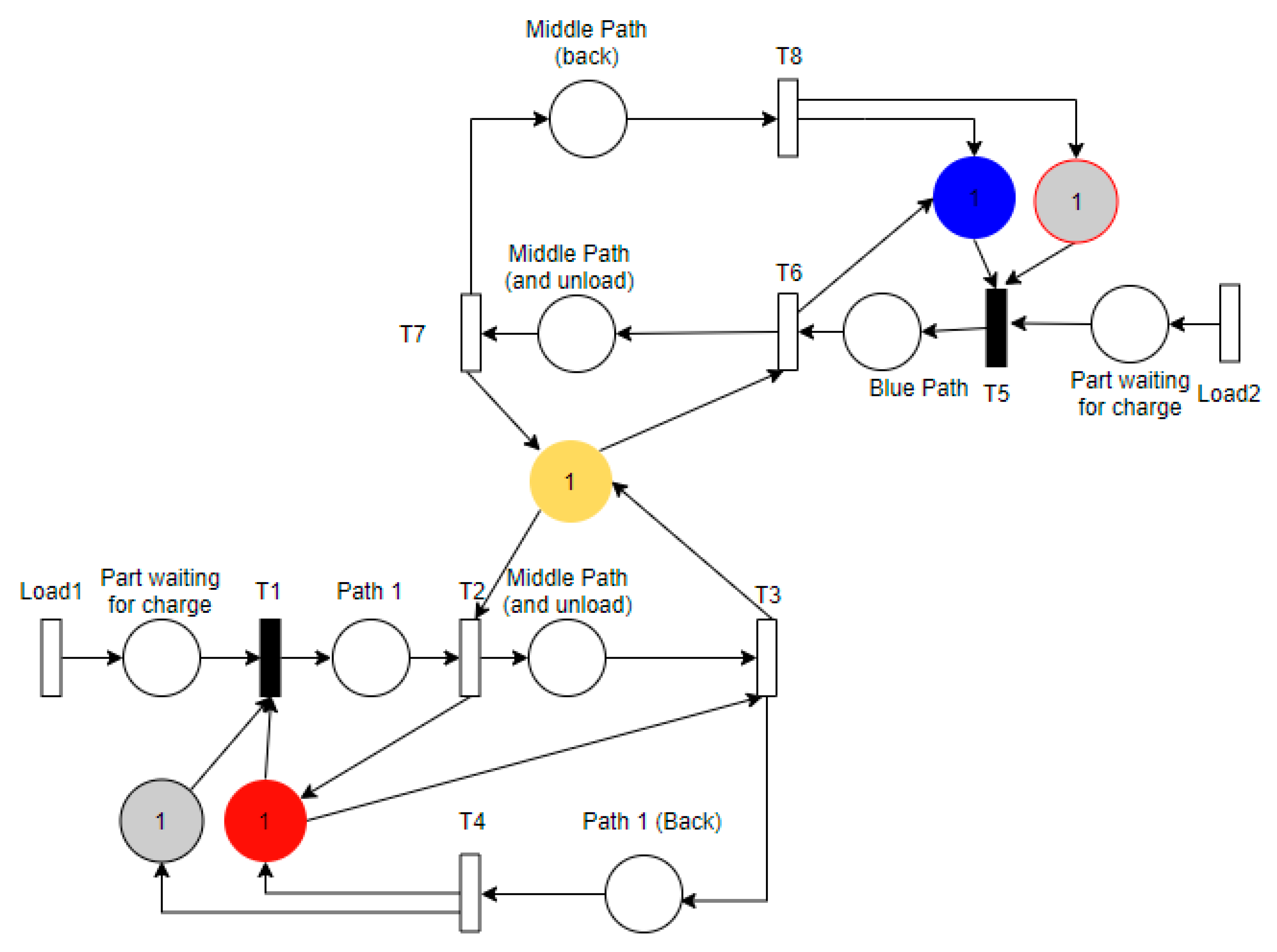
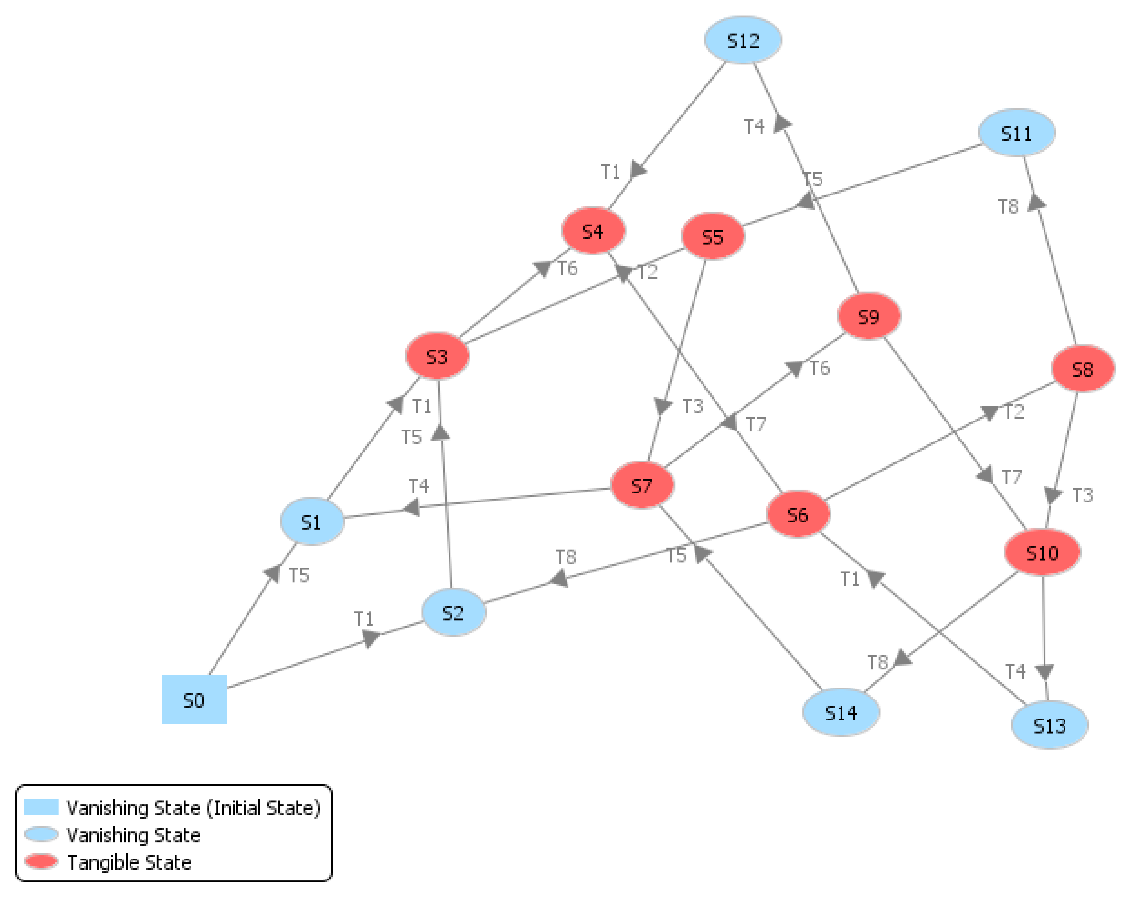
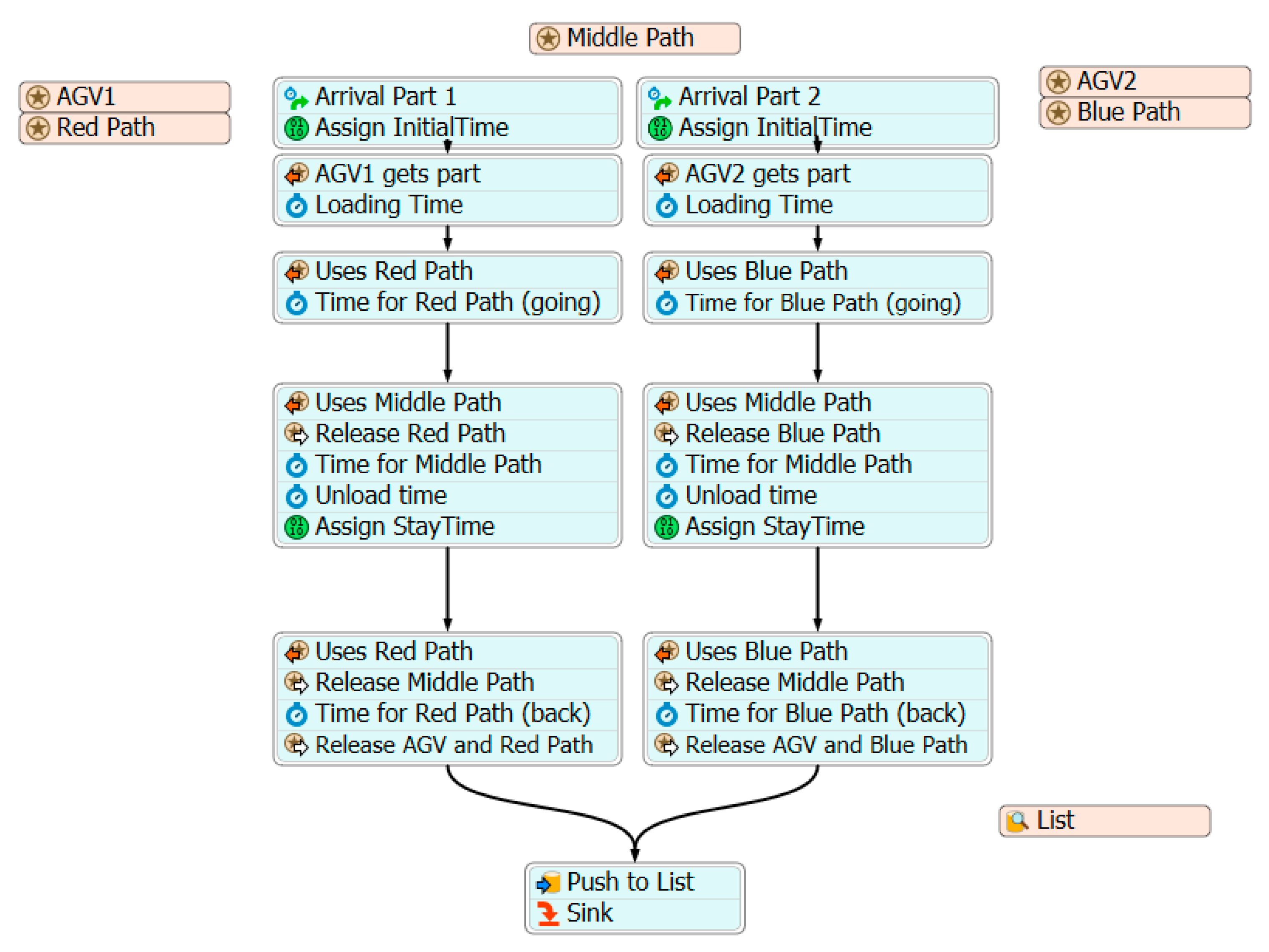
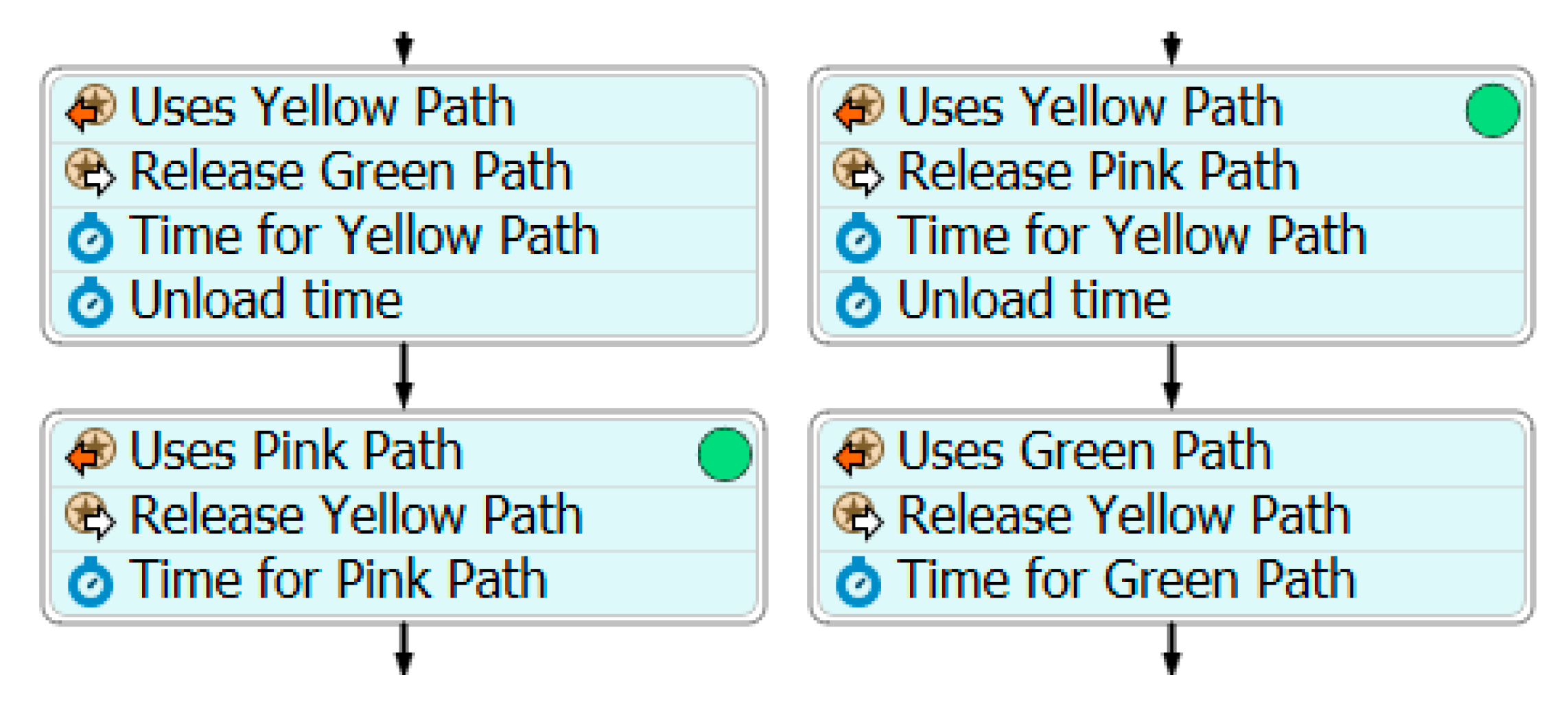
6. Example: Bridge Crossing Deadlock

In this example, we analyze the use of Petri nets to detect a deadlock (using an AGV example) before encoding the resulting scenarios in FlexSim. The most basic deadlocks in AGV systems would be when two of the vehicles use the same bidirectional lane but travel in opposite directions. An example of this is shown in Figure 14.

In this example, AGV1 needs to move cargo from Load1 to Unload1 and analogously for AGV2. Eventually, AGV1 and AGV2 may enter the same lane from opposite sides, blocking the whole system. This situation arises because AGV1 wants to access Unload1 and AGV2 wants to access Unload2, but they cannot collide or pass over one another, leaving us with two vehicles that want to move but whose paths are blocked.

6.1. Petri Net Model

The case shown in Figure 12 can be transformed into a Petri net. While one AGV covers part of the tracks, the other AGV cannot. Ideally, every inch of the tracks should be a resource, but this is not helpful. Therefore, the representation is divided into different sections according to their use by the AGVs. The different paths are divided as shown in Figure 15, where they are represented with different colors.

Now that each path has been labeled, the Petri net can be constructed as shown in Figure 16.

In this case, we had to assume that there is just one part waiting to be loaded at both load stations; when it returns it waits to be loaded again so it can be represented in the PIPE simulator. Figure 17 shows the different terminal states in which two different systems can be found (S10 and S11).

The corresponding deadlocks are represented in Figure 18. Note that it is particularly easy to interpret the problem of two vehicles on a one-lane bridge: they cannot use it at the same time because they are traveling in opposite directions.

There are only two deadlock situations because the bridge has been divided into three sections.

Alternative 1: Avoiding Deadlock

The system becomes deadlocked if both AGVs attempt to use the middle path at the same time from opposite sides. One possible solution is, for the first AGV to reach the middle path road, traps all the resources until the vehicle departs. The other AGV, if idle, must wait until the first vehicle releases the resource. The new Petri pet is displayed in Figure 19.

Note that the different sub-paths (green, yellow, and pink) no longer exist. This is because in the new situation it does not make sense to describe the path as three different resources since one catches them all up at the same time. The corresponding reachability graph can be seen in Figure 20, which shows that the system is totally cyclical and, therefore, not susceptible to deadlocks.

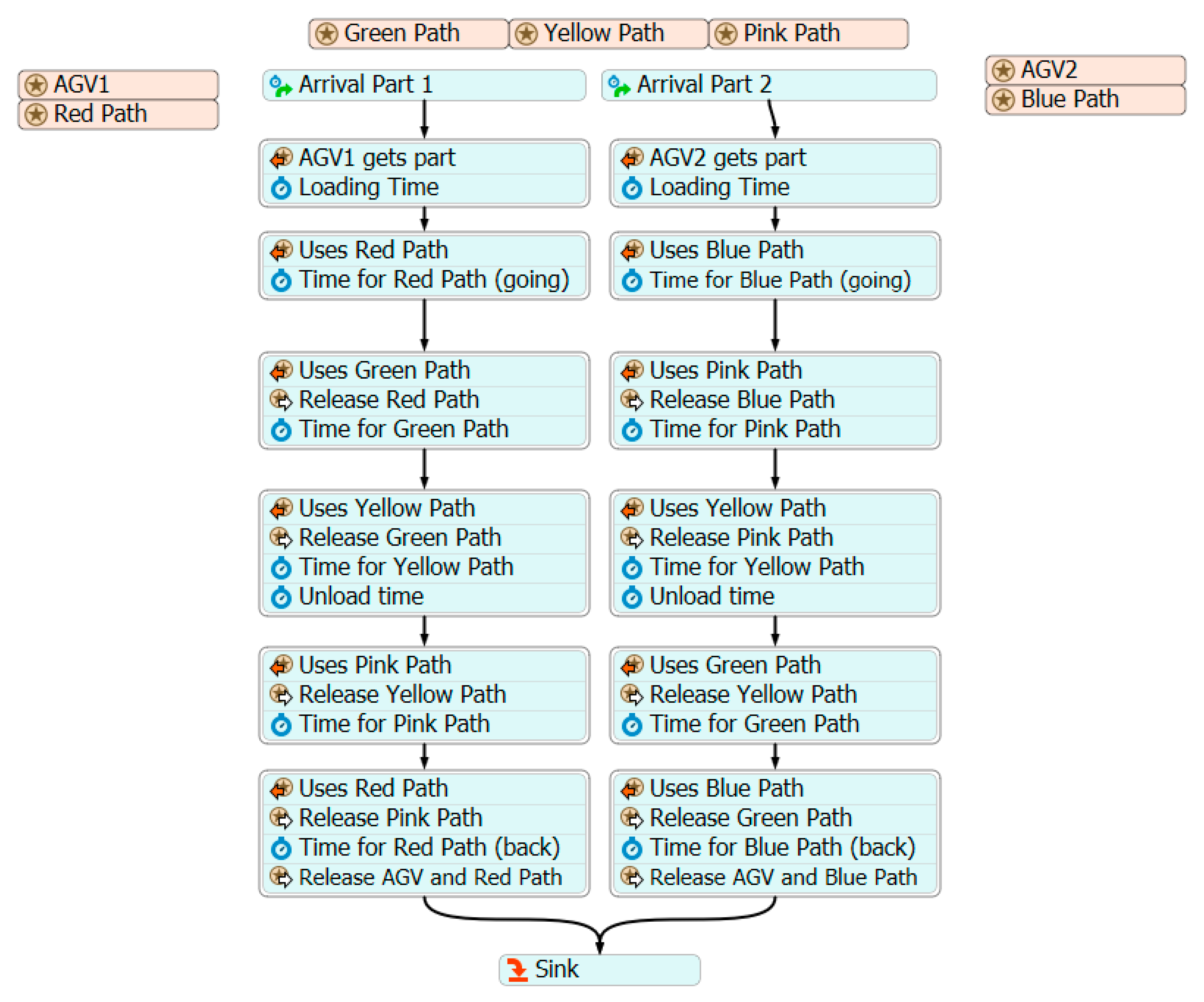
6.2. FlexSim Process Simulation Flow

The two proposed solutions need to be simulated in FlexSim to obtain results for different state systems so that they can be compared. This is different to the previous cases, as there are two possible alternatives to prevent deadlocks: (i) original case (possible deadlock) and (ii) solution (blocking the middle path with only one AGV), see Figure 21 for the original case with possible deadlock, and Figure 22 for the proposed solution (blocking the middle path).

7. Discussion

Static analysis of the two Petri nets reveals a deadlock at design time, through the analysis of the reachability graph. By encoding the two alternatives and performing an execution with non-validated systemic data assumptions, we can see that the first model is very likely to lead to a deadlock in the system. If both AGVs enter the bridge at the same time, the problem occurs in FlexSim and the process cannot continue, as shown in Figure 23.

In this case, is clear that the analysis of the conceptual model allows detection of behavior in the system (that can be known by the stakeholders of the system or not). This implies that the conceptual model itself can be considered as a valuable tool, not only for the documentation of the model and to allow multiple codifications, but also to understand and to validate the assumptions we use for modeling.

8. Conclusions

The conceptualization of a simulation model is a necessary task that sometimes is not undertaken because of the constraints in the time needed to finish the project or because of a misunderstanding in the differentiation between the model and the codification of the model. However, the conceptualization of a simulation model is a key aspect for undertaking the validation process and to detect, as is shown here, some issues in the system structure prior to any execution of the simulation model. For this reason, the conceptual model can be considered a product in itself [47], being a central element in the validation, verification and accreditation cycle [48,49].

This paper has shown how we can use a widely used formalism, the Petri net, to define a conceptual model and from it, following the proposed mapping, systematically obtain the codification for a FlexSim platform. This process reduces the change to introduce errors due to the codification process, implying a reduction in the time needed to undertake the verification of the FlexSim simulation model.

Since FlexSim allows extension and personalization of the behavior of the objects in question, one can use this mapping to create a library that automatically does this mapping, allowing the code to be obtained in a shorter time and with few errors, keeping the distinction between the conceptual model, and allowing all the advantages of the conceptual model to be obtained, like the possibility of an analysis prior to any codification and the possibility to reimplement the model in other tools. Also, this mapping allows existing Petri net models to use a commercial and powerful tool like FlexSim to perform the codifications of its models.

References

1. Doldi, L. SDL Illustrated-Visually Design Executable Models; MSO Systems: Old Main, PA, USA, 2001. [Google Scholar]
2. ITU-T. Specification and Description Language–Overview of SDL-2010; ITU-T: Geneva, Switzerland, 2011. [Google Scholar]
3. Guasch, A.; Figueras, J.; Casanovas, J. Conceptual modeling using Petri Nets. In Formal Languages Forcomputer Simulation: Transdisciplinary Models and Applications; IGI Global: Hershey, PA, USA, 2013. [Google Scholar]
4. Cabasino, M.P.; Giua, A.; Seatzu, C. Introduction to petri nets. Lect. Notes Control Inf. Sci. 2013, 433, 191–211. [Google Scholar] [CrossRef]
5. Van der Aalst, W.M.P. Timed Coloured Petri Nets and Their Application to Logistics. Ph.D. Thesis, Technische Universiteit Eindhoven, Eindhoven, The Netherlands, 1992. [Google Scholar] [CrossRef]
6. Zeigler, B.P.; Praehofer, H.; Kim, T.G. Theory of Modeling and Simulation Handbook of Simulator-BASED Training Creating Computer Simulation Systems: An Introduction to the High Level Architecture; Academic Press: Oxford, UK, 2000. [Google Scholar] [CrossRef]
7. Vangheluwe, H.L.M. DEVS as a common denominator for multi-formalism hybrid systemsmodelling. CACSD. In Proceedings of the IEEE International Symposium on Computer-Aided Control System Design (Cat. No.00TH8537), Anchorage, AK, USA, 25–27 September 2000. [Google Scholar]
8. Fonseca i Casas, P. Transforming classic Discrete Event System Specification models to Specification and Description Language. Simulation 2015, 91, 249–264. [Google Scholar] [CrossRef]
9. Boukelkoul, S.; Redjimi, M. Mapping between Petri nets and DEVS models. In Proceedings of the 2013 3rd International Conference on Information Technology and e-Services (ICITeS), Sousse, Tunisia, 24–26 March 2013; pp. 1–6. [Google Scholar] [CrossRef]
10. Sargent, R. Verification and validation of simulation models. In Proceedings of the 2009 Winter Simulation Conference (WSC); Rossetti, M.D., Hill, R.R., Johansson, B., Dunkin, A., Ingalls, R.G., Eds.; WSC: Austin, TX, USA, 2009; p. 66. [Google Scholar] [CrossRef] [Green Version]
11. Van Bruggen, A.; Nikolic, I.; Kwakkel, J. Modeling with stakeholders for transformative change. Sustainability 2019, 11, 825. [Google Scholar] [CrossRef] [Green Version]
12. Brailsford, S.C.; Bolt, T.; Connell, C.; Klein, J.H.; Patel, B. Stakeholder engagement in health care simulation. Proc.-Winter Simul. Conf. 2009, 1840–1849. [Google Scholar] [CrossRef] [Green Version]
13. Proudlove, N.C.; Bisogno, S.; Onggo, B.S.S.; Calabrese, A.; Levialdi Ghiron, N. Towards fully-facilitated discrete event simulation modelling: Addressing the model coding stage. Eur. J. Oper. Res. 2017, 263, 583–595. [Google Scholar] [CrossRef] [Green Version]
14. Onggo, B.S.S.; Proudlove, N.C.; D’Ambrogio, S.A.; Calabrese, A.; Bisogno, S.; Levialdi Ghiron, N. A BPMN extension to support discrete-event simulation for healthcare applications: An explicit representation of queues, attributes and data-driven decision points. J. Oper. Res. Soc. 2018, 69, 788–802. [Google Scholar] [CrossRef] [Green Version]
15. Aagesen, G.; Krogstie, J. BPMN 2.0 for Modeling Business Processes. In Handbook on Business Process Management 1; Springer: Berlin/Heidelberg, Germany, 2015; pp. 219–250. [Google Scholar] [CrossRef]
16. Leiva, J.; Fonseca i Casas, P.; Ocana, J. Modeling anesthesia and pavilion surgical units in a Chilean hospital with Specification and Description Language. Simulation 2013, 89, 1020–1035. [Google Scholar] [CrossRef]
17. Fonseca i Casas, P. SDL distributed simulator. In 2008 Winter Simulation Conference; Winter Simulation Conference: Miami, FL, USA, 2008. [Google Scholar] [CrossRef]
18. PragmaDev SARL. PragmaDev Studio. Available online: http://www.pragmadev.com/product/index.html (accessed on 15 February 2020).
19. Wainer, G.A. Modeling and simulation of complex systems with cell-DEVS. In Proceedings of the 2004 Winter Simulation Conference, Washington, DC, USA, 5–8 December 2004; Ingalls, R.G., Rossett, M.D., Smith, J.S., Peters, B.A., Eds.; Winter Simulation Conference: Washington, DC, USA, 2004. [Google Scholar]
20. López, J.; Santana-Alonso, A.; Medina, M.D.C. Formal verification for task description languages. A petri net approach. Sensors (Switzerland) 2019, 19, 4965. [Google Scholar] [CrossRef] [Green Version]
21. Kucera, E.; Haffner, O.; Leskovsky, R. PN2ARDUINO—A new petri net software tool for control of discrete-event and hybrid systems using arduino microcontrollers. Proc. 2019 Fed. Conf. Comput. Sci. Inf. Syst. FedCSIS 2019, 18, 915–919. [Google Scholar] [CrossRef]
22. Peleg, M.; Rubin, D.; Altman, R.B. Using Petri Net tools to study properties and dynamics of biological systems. J. Am. Med. Inform. Assoc. 2005, 12, 181–199. [Google Scholar] [CrossRef] [Green Version]
23. Liang, X.; Zhang, S.; Liu, Y.; Ma, Y. Information Propagation Formalized Representation of Micro-blog Network Based on Petri Nets. Sci. Rep. 2020, 10, 1–20. [Google Scholar] [CrossRef] [PubMed] [Green Version]
24. Balogh, Z.; Kuchárik, M. Predicting student grades based on their usage of LMS moodle using Petri nets. Appl. Sci. 2019, 9, 4211. [Google Scholar] [CrossRef] [Green Version]
25. Su, Z.; Qiu, M. Airport surface modelling and simulation based on timed coloured petri net. Promet-Traffic -Traffico. 2019, 31, 479–490. [Google Scholar] [CrossRef]
26. Tolba, C.; Lefebvre, D.; Thomas, P.; El Moudni, A. Continuous and timed Petri nets for the macroscopic and microscopic traffic flow modelling. Simul. Model. Pract. Theory 2005, 13, 407–436. [Google Scholar] [CrossRef]
27. An, Y.; Wu, N.; Zhao, X.; Li, X.; Chen, P. Hierarchical Colored Petri nets for modeling and analysis of transit signal priority control systems. Appl. Sci. 2018, 8, 141. [Google Scholar] [CrossRef] [Green Version]
28. Meghzili, S.; Chaoui, A.; Strecker, M.; Kerkouche, E. An Approach for the Transformation and Verification of BPMN Models to Colored Petri Nets Models. Int. J. Softw. Innov. 2020, 8, 17–49. [Google Scholar] [CrossRef]
29. Gulati, U.; Vatanawood, W. Transforming Flowchart into Coloured Petri Nets. In Proceedings of the 2019 3rd International Conference on Software and e-Business; ACM: New York, NY, USA, 2019; pp. 75–80. [Google Scholar] [CrossRef]
30. Mutarraf, U.; Barkaoui, K.; Li, Z.; Wu, N.; Qu, T. Transformation of Business Process Model and Notation models onto Petri nets and their analysis. Adv. Mech. Eng. 2018, 10, 1–21. [Google Scholar] [CrossRef]
31. Haustermann, M. Petri Nets Tool Database. Available online: https://www.informatik.uni-hamburg.de/TGI/PetriNets/tools/db.html (accessed on 15 February 2020).
32. Abohamad, W.; Ramy, A.; Arisha, A. A Hybrid Process-Mining Approach for Simulation Modeling. In Proceedings of the 2017 Winter Simulation Conference; Winter Simulation Conference: Las Vegas, NV, USA, 2017. [Google Scholar] [CrossRef] [Green Version]
33. Bergmann, S.; Strassburger, S. Challenges for the Automatic Generation of Simulation Models for Production Systems. In Proceedings of the 2010 Summer Computer Simulation Conference, Ottawa, ON, Canada, 11–14 July 2010; SCSC: Ottawa, ON, Canada, 2010; pp. 545–549. [Google Scholar]
34. Santillán Martínez, G.; Sierla, S.A.; Karhela, T.A.; Lappalainen, J.; Vyatkin, V. Automatic Generation of a High-Fidelity Dynamic Thermal-Hydraulic Process Simulation Model From a 3D Plant Model. IEEE Access. 2018, 6, 45217–45232. [Google Scholar] [CrossRef]
35. Dias, L.M.S.; Vieira, A.A.C.; Oliveira, G.A.B.P.J.A. Discrete Simulation Software Ranking—A Top List of the Worldwide Most Popular and Used Tools. Proc. 2016 Winter Simul. Conf. 2016, 53, 1689–1699. [Google Scholar] [CrossRef]
36. Huang, B.; Tang, H. Study of Workshop Production System Based on Petri Nets and Flexsim. In Proceedings of the 22nd International Conference on Industrial Engineering and Engineering Management 2015; Qi, E., Shen, J., Dou, R., Eds.; Atlantis Press: Paris, France, 2016; pp. 833–844. [Google Scholar] [CrossRef]
37. Xu, S.Z. A Petri Net-Based Hybrid Heuristic Scheduling Algorithm for Flexible Manufacturing System. Int. J. Simul. Model. 2019, 18, 325–334. [Google Scholar] [CrossRef]
38. Altiok, T.; Melamed, B. Simulation Modeling and Analysis with ARENA; Elsevier: Piscataway, NJ, USA, 2007. [Google Scholar]
39. Figueras, J.I.J.; Guasch, A.I.P.; Fonseca, P.I.C.; Casanovas-Garcia, J. Teaching system modelling and simulation through Petri Nets and Arena. In Proceedings of the Winter Simulation Conference, Savanah, GA, USA, 7–10 December 2014; pp. 3662–3673. [Google Scholar] [CrossRef]
40. Wang, J. Petri Nets for Dynamic Event-Driven System Modeling. In Handbook of Dynamic System Modeling; Fishwick, P.A., Ed.; Chapman & Hall: Gainesville, FL, USA, 2007; pp. 17–24. [Google Scholar] [CrossRef]
41. Dingle, N.; Knottenbelt, W.; Suto, T. PIPE2: a tool for the performance evaluation of generalised stochastic Petri Nets. ACM SIGMETRICS Perform. Eval. Rev. 2009, 36, 34. [Google Scholar] [CrossRef]
42. Bonet, P.; Lladó, C. PIPE v2. 5: A Petri net tool for performance modelling. In Proceedings of the 23rd Latin American Conference on Informatics (CLEI 2007), Osijek, Croatia, 9–12 October 2007; Faculty of Law, Josip Juraj Strossmayer University in Osijek: Osijek, Croatia, 2007; Volume 12. [Google Scholar]
43. FlexSim Software Products Inc. FlexSim Problem Solved. Available online: https://www.flexsim.com/ (accessed on 15 February 2020).
44. Law, A.M.; Kelton, W. Simulation Modeling and Analysis; McGraw-Hill: New York, NY, USA, 2000. [Google Scholar]
45. OPC Foundation. Unified Architecture. Available online: https://opcfoundation.org/about/opc-technologies/opc-ua/ (accessed on 15 February 2020).
46. Pels, H.J.; Goossenaerts, J. A Conceptual Modeling Technique for Discrete Event Simulation of Operational Processes. In Advances in Production Management Systems; Springer: Boston, MA, USA, 2007; pp. 305–312. [Google Scholar] [CrossRef] [Green Version]
47. Sargent, R.G. Verification and validation of simulation models. J. Simul. 2013, 7, 12–24. [Google Scholar] [CrossRef] [Green Version]
48. Chew, J.; Sullivan, C. Verification, validation, and accreditation in the life cycle of models and simulations. In 2000 Winter Simulation Conference Proceedings; Winter Simulation Conference: San Diego, CA, USA, 2000; pp. 813–818. [Google Scholar]
49. Balci, O. Golden rules of verification, validation, testing, and certification of modeling and simulation applications. SCS M S Mag. 2010, 4, 1–7. [Google Scholar]
Figure 1. Simplified modeling process for a simulation project [10], showing in red the aspects that will be affected by the proposed methodology. The conceptual model-tool mapping simplifies the verification process and encoding.
Applsci 10 01395 g001
Figure 2. Example of a basic Petri net.
Applsci 10 01395 g002
Figure 3. Graphical representation of an immediate (top) and a timed transition (bottom).
Applsci 10 01395 g003
Figure 4. FlexSim environment with a basic model. The construction of the model is based on the selection of the elements that are presented on the left side and the configuration of those elements on the right side of the environment.
Applsci 10 01395 g004
Figure 5. Sequential execution in Petri net (left) and FlexSim (right).
Applsci 10 01395 g005
Figure 6. Conflict in Petri net (left) and FlexSim (right).
Applsci 10 01395 g006
Figure 7. Example of a deterministic decision with FlexSim (label version).
Applsci 10 01395 g007
Figure 8. Example of a deterministic decision with FlexSim (conditional version).
Applsci 10 01395 g008
Figure 9. Example of a probabilistic decision with FlexSim.
Applsci 10 01395 g009
Figure 10. Concurrency with temporal entities in FlexSim.
Applsci 10 01395 g010
Figure 11. Synchronization with temporal entities in FlexSim.
Applsci 10 01395 g011
Figure 12. Petri net for a queue-server model.
Applsci 10 01395 g012
Figure 13. Resource activities in FlexSim.
Applsci 10 01395 g013
Figure 14. Case IV: Screenshot of the bridge crossing deadlock problem represented in FlexSim.
Applsci 10 01395 g014
Figure 15. Case IV: different sectors for the automatic guided vehicle (AGV) network.
Applsci 10 01395 g015
Figure 16. Case IV: initial marking of Petri net.
Applsci 10 01395 g016
Figure 17. Case IV: reachability/coverability graph obtained by PIPE simulator.
Applsci 10 01395 g017
Figure 18. Case IV: deadlocks represented in Petri nets (S10 on the left, S11 on the right).
Applsci 10 01395 g018
Figure 19. Case IV: proposed deadlock solution (blocking the middle path).
Applsci 10 01395 g019
Figure 20. Case IV: reachability/coverability graph obtained by the PIPE simulator for the first proposed solution.
Applsci 10 01395 g020
Figure 21. Encoding of both Petri nets in FlexSim. The original case (possible deadlock).
Applsci 10 01395 g021
Figure 22. Encoding of both Petri nets in FlexSim. Proposed solution (blocking the middle path).
Applsci 10 01395 g022
Figure 23. Deadlock represented in FlexSim.
Applsci 10 01395 g023