A Hybrid Degradation Modeling and Prognostic Method for the Multi-Modal System

 ,
, 

Abstract
1. Introduction
2. Degradation Modeling and Prognostic Hybrid
2.1. Long-Term Cumulative Degradation Assessment with Cdd-Hi
2.1.1. Cumulative Dynamic Difference Feature Extraction
2.1.2. Composite Health Indicator Construction
2.1.3. Cumulative Degradation Assessment with Gated Recurrent Unit
2.2. Latest-Term Degradation Assessment Based on Local Features
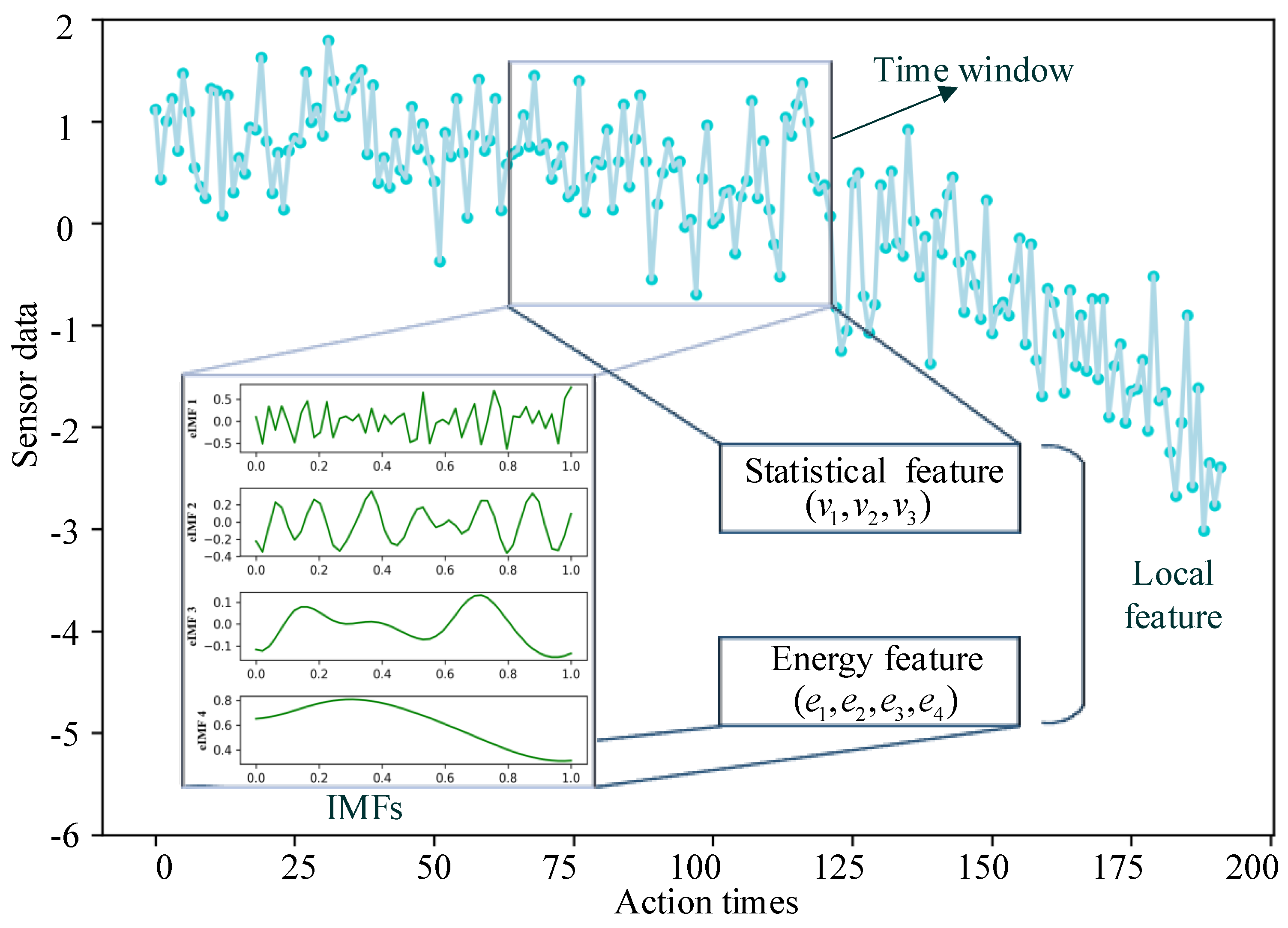
2.2.1. Construction of Local Aging Features
2.2.2. Latest-Term Degradation Assessment Based on Local Features and LightGBM
2.3. Decision-Level Fusion Based on Model Averaging
3. Experiment and Discussion
3.1. Evaluation Metrics
3.2. Theoretical Analysis
3.3. Experimental Simulation
3.3.1. Benchmark Data Description
3.3.2. Data Preprocessing
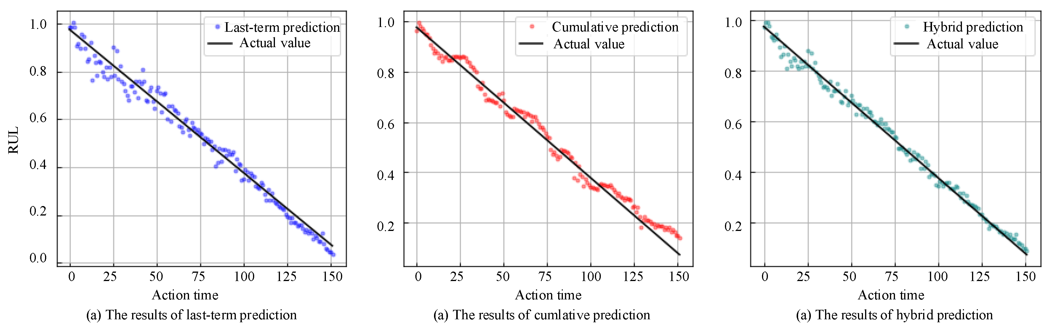
3.3.3. Discussion of Results
4. Conclusions
Author Contributions
Funding
Acknowledgments
Conflicts of Interest
Abbreviations
| RUL | Remainning useful life |
| HI | Health indicator |
| CDD-HI | Cumulative dynamic differential health indicator |
| GBDT | Gradient boosting decision tree |
| LightGBM | Light gradient boosting machine |
| RNN | Recurrent neural network |
| GRU | Gated recurrent unit |
| DTW | Dynamic time warping |
| LSTM | Long-short term memory network |
| EEMD | Ensemble empirical mode decomposition |
| IMF | Intrinsic mode function |
| CNN | Convolutional neural networks |
| SVR | Support vector regression |
| SAEs | Stacked autoencodesrs |
References
- Zhang, C.; Lim, P.; Qin, A.K.; Tan, K.C. Multiobjective deep belief networks ensemble for remaining useful life estimation in prognostics. IEEE Trans. Neural Networks Learn. Syst. 2016, 28, 2306–2318. [Google Scholar] [CrossRef]
- Yang, D. Physics-of-failure-based prognostics and health management for electronic products. In Proceedings of the 2014 15th International Conference on Electronic Packaging Technology (ICEPT2014), Chengdu, China, 12–15 August 2014; pp. 1215–1218. [Google Scholar]
- Huang, B.; Cohen, K.; Zhao, Q. Active anomaly detection in heterogeneous processes. In Proceedings of the 2018 International Conference on Acoustics, Speech, and Signal Processing (ICASSP2018), Calgary, AB, Canada, 15–20 April; pp. 3924–3928.
- Li, N.; Lei, Y.; Guo, L.; Yan, T.; Lin, J. Remaining useful life prediction based on a general expression of stochastic process models. IEEE Trans. Ind. Electron. 2017, 64, 5709–5718. [Google Scholar] [CrossRef]
- Kang, M.; Kim, J.; Kim, J.M. Reliable fault diagnosis for low-speed bearings using individually trained support vector machines with kernel discriminative feature analysis. IEEE Trans. Power Electron. 2014, 30, 2786–2797. [Google Scholar] [CrossRef]
- Xiao, L.; Chen, X.; Zhang, X.; Liu, M. A novel approach for bearing remaining useful life estimation under neither failure nor suspension histories condition. J. Intell. Manuf. 2017, 28, 1893–1914. [Google Scholar] [CrossRef]
- Glowacz, A.; Glowacz, Z. Diagnosis of stator faults of the single-phase induction motor using acoustic signals. Appl. Acoust. 2017, 117, 20–27. [Google Scholar] [CrossRef]
- Huang, B.; Cohen, K.; Zhao, Q. Active anomaly detection in heterogeneous processes. IEEE Trans. Inf. Theory 2018, 65, 2284–2301. [Google Scholar] [CrossRef]
- Zio, E.; Di Maio, F. A data-driven fuzzy approach for predicting the remaining useful life in dynamic failure scenarios of a nuclear system. Reliab. Eng. Syst. Saf. 2010, 95, 49–57. [Google Scholar] [CrossRef]
- Cheng, Y.; Peng, J.; Gu, X.; Zhang, X.; Liu, W.; Yang, Y.; Huang, Z. RLCP: A Reinforcement Learning Method for Health Stage Division Using Change Points. In Proceedings of the 2018 IEEE International Conference on Prognostics and Health Management (ICPHM2014), Seattle, WA, USA, 11–13 June 2018; pp. 1–6. [Google Scholar]
- Yang, Y.; Xiong, L.; Liu, W.; Gao, K.; Huang, Z. An Energy-Based Nonlinear Pressure Observer for Fast and Precise Braking Force Control of the ECP Brake. Int. J. Precis. Eng. Manuf. 2018, 19, 1437–1445. [Google Scholar] [CrossRef]
- Li, H.; Zhang, X.; Peng, J.; He, J.; Huang, Z.; Wang, J. Cooperative CC-CV charging of supercapacitors using multi-charger systems. IEEE Trans. Ind. Electron. 2020. [Google Scholar] [CrossRef]
- Wu, Y.; Yuan, M.; Dong, S.; Lin, L.; Liu, Y. Remaining useful life estimation of engineered systems using vanilla LSTM neural networks. Neurocomputing 2018, 275, 167–179. [Google Scholar] [CrossRef]
- Khelif, R.; Chebel-Morello, B.; Malinowski, S.; Laajili, E.; Fnaiech, F.; Zerhouni, N. Direct remaining useful life estimation based on support vector regression. IEEE Trans. Ind. Electron. 2016, 64, 2276–2285. [Google Scholar] [CrossRef]
- Zheng, S.; Ristovski, K.; Farahat, A.; Gupta, C. Long short-term memory network for remaining useful life estimation. In Proceedings of the 2017 IEEE International Conference on Prognostics and Health Management (ICPHM 2017), Chiba, Japan, 13–17 April 2018; pp. 88–95. [Google Scholar]
- Hu, C.; Youn, B.D.; Wang, P.; Yoon, J.T. Ensemble of data-driven prognostic algorithms for robust prediction of remaining useful life. Reliab. Eng. Syst. Saf. 2012, 103, 120–135. [Google Scholar] [CrossRef]
- Lei, Y.; Li, N.; Guo, L.; Li, N.; Yan, T.; Lin, J. Machinery health prognostics: A systematic review from data acquisition to RUL prediction. Mech. Syst. Signal Process. 2018, 104, 799–834. [Google Scholar] [CrossRef]
- Liao, H.; Tian, Z. A framework for predicting the remaining useful life of a single unit under time-varying operating conditions. Iie Trans. 2013, 45, 964–980. [Google Scholar] [CrossRef]
- Lei, Y.; Li, N.; Lin, J. A new method based on stochastic process models for machine remaining useful life prediction. IEEE Trans. Instrum. Meas. 2016, 65, 2671–2684. [Google Scholar] [CrossRef]
- Li, H.; Wang, Y.; Wang, B.; Sun, J.; Li, Y. The application of a general mathematical morphological particle as a novel indicator for the performance degradation assessment of a bearing. Mech. Syst. Signal Process. 2017, 82, 490–502. [Google Scholar] [CrossRef]
- Hu, J.; Tse, P. A relevance vector machine-based approach with application to oil sand pump prognostics. Sensors 2013, 13, 12633–12686. [Google Scholar] [CrossRef]
- Benkedjouh, T.; Medjaher, K.; Zerhouni, N.; Rechak, S. Health assessment and life prediction of cutting tools based on support vector regression. J. Intell. Manuf. 2015, 26, 213–223. [Google Scholar] [CrossRef]
- Lei, Y.; Li, N.; Gontarz, S.; Lin, J.; Radkowski, S.; Dybala, J. A model-based method for remaining useful life prediction of machinery. IEEE Trans. Reliab. 2016, 65, 1314–1326. [Google Scholar] [CrossRef]
- Guo, L.; Li, N.; Jia, F.; Lei, Y.; Lin, J. A recurrent neural network based health indicator for remaining useful life prediction of bearings. Neurocomputing 2017, 240, 98–109. [Google Scholar] [CrossRef]
- Zhang, Y.; Xiong, R.; He, H.; Liu, Z. A lstm-rnn method for the lithuim-ion battery remaining useful life prediction. In Proceedings of the 2017 Prognostics and System Health Management Conference (PHM-Harbin 2017), Harbin, China, 9–12 July 2017; pp. 1–4. [Google Scholar]
- Song, Y.; Li, L.; Peng, Y.; Liu, D. Lithium-Ion Battery Remaining Useful Life Prediction Based on GRU-RNN. In Proceedings of the 2018 12th International Conference on Reliability, Maintainability, and Safety (ICRMS 2018), Shanghai, China, 17–19 October 2018; pp. 317–322. [Google Scholar]
- Zheng, C.; Liu, W.; Chen, B.; Gao, D.; Cheng, Y. A data-driven approach for remaining useful life prediction of aircraft engines. In Proceedings of the 2018 21st International Conference on Intelligent Transportation Systems (ITSC 2018), Maui, HI, USA, 4–7 November 2018; pp. 184–189. [Google Scholar]
- Wang, S.; Zhang, X.; Gao, D.; Chen, B.; Cheng, Y.; Yang, Y.; Peng, J. A Remaining Useful Life Prediction Model Based on Hybrid Long-Short Sequences for Engines. In Proceedings of the 2018 21st International Conference on Intelligent Transportation Systems (ITSC 2018), Maui, HI, USA, 4–7 November 2018; pp. 1757–1762. [Google Scholar]
- Singh, S.K.; Kumar, S.; Dwivedi, J.P. A novel soft computing method for engine RUL prediction. Multimed. Tools Appl. 2019, 78, 4065–4087. [Google Scholar] [CrossRef]
- Chen, T.; Guestrin, C. Xgboost: A scalable tree boosting system. In Proceedings of the 2016 22nd ACM Sigkdd International Conference on Knowledge Discovery and Data Mining (ACM 2016), Amsterdam, The Netherlands, 15–19 October 2016; pp. 785–794. [Google Scholar]
- Ke, G.; Meng, Q.; Finley, T. Lightgbm: A highly efficient gradient boosting decision tree. In Proceedings of the Advances in Neural Information Processing Systems (NIPS 2017), Long Beach, CA, USA, 3–9 December 2017; pp. 3146–3154. [Google Scholar]
- Mosallam, A.; Medjaher, K.; Zerhouni, N. Data-driven prognostic method based on Bayesian approaches for direct remaining useful life prediction. J. Intell. Manuf. 2016, 27, 1037–1048. [Google Scholar] [CrossRef]
- Pan, Y.; Er, M.J.; Li, X. Machine health condition prediction via online dynamic fuzzy neural networks. Eng. Appl. Artif. Intell. 2014, 35, 105–113. [Google Scholar] [CrossRef]
- Liao, L.; Köttig, F. Review of hybrid prognostics approaches for remaining useful life prediction of engineered systems, and an application to battery life prediction. IEEE Trans. Reliab. 2014, 63, 191–207. [Google Scholar] [CrossRef]
- Bengio, Y.; Simard, P.; Frasconi, P. Learning long-term dependencies with gradient descent is difficult. IEEE Trans. Neural Networks 1994, 5, 157–166. [Google Scholar] [CrossRef] [PubMed]
- Zhang, X.; Xiao, P.; Yang, Y. Remaining Useful Life Estimation Using CNN-XGB with Extended Time Window. IEEE Access 2019, 7, 15438–154397. [Google Scholar] [CrossRef]
- Coble, J.B.; Hines, J.W. Prognostic algorithm categorization with PHM challenge application. In Proceedings of the 2008 International Conference on Prognostics and Health Management (ICPHM2008), Denver, CO, USA, 6–9 October 2008; pp. 1–11. [Google Scholar]
- Saxena, A.; Goebel, K.; Simon, D. Damage propagation modeling for aircraft engine run-to-failure simulation. In Proceedings of the 2008 International Conference on Prognostics and Health Management (ICPHM2008), Denver, CO, USA, 6–9 October 2008; pp. 1–9. [Google Scholar]
- Frederick, D.K.; DeCastro, J.A.; Litt, J.S. User’s Guide for the Commercial Modular Aero-Propulsion System Simulation (C-MAPSS); NASA Glenn Research Center: Cleveland, OH, USA, 2007.
- Saxena, A.; Goebel, K. Turbofan Engine Degradation Simulation Data Set. NASA Ames Prognostics Data Repository. 2008. Available online: https://ti.arc.nasa.gov/tech/dash/groups/pcoe/prognostic-datarepository/ (accessed on 20 November 2018).
- Wold, S.; Esbensen, K.; Geladi, P. Principal component analysis. Chemom. Intell. Lab. Syst. 1987, 2, 37–52. [Google Scholar] [CrossRef]


| Parameter | No. 1 | No. 2 | No. 3 | No. 4 | No. 5 | No. 6 | No. 7 | No. 8 | No. 9 | No. 10 | |
|---|---|---|---|---|---|---|---|---|---|---|---|
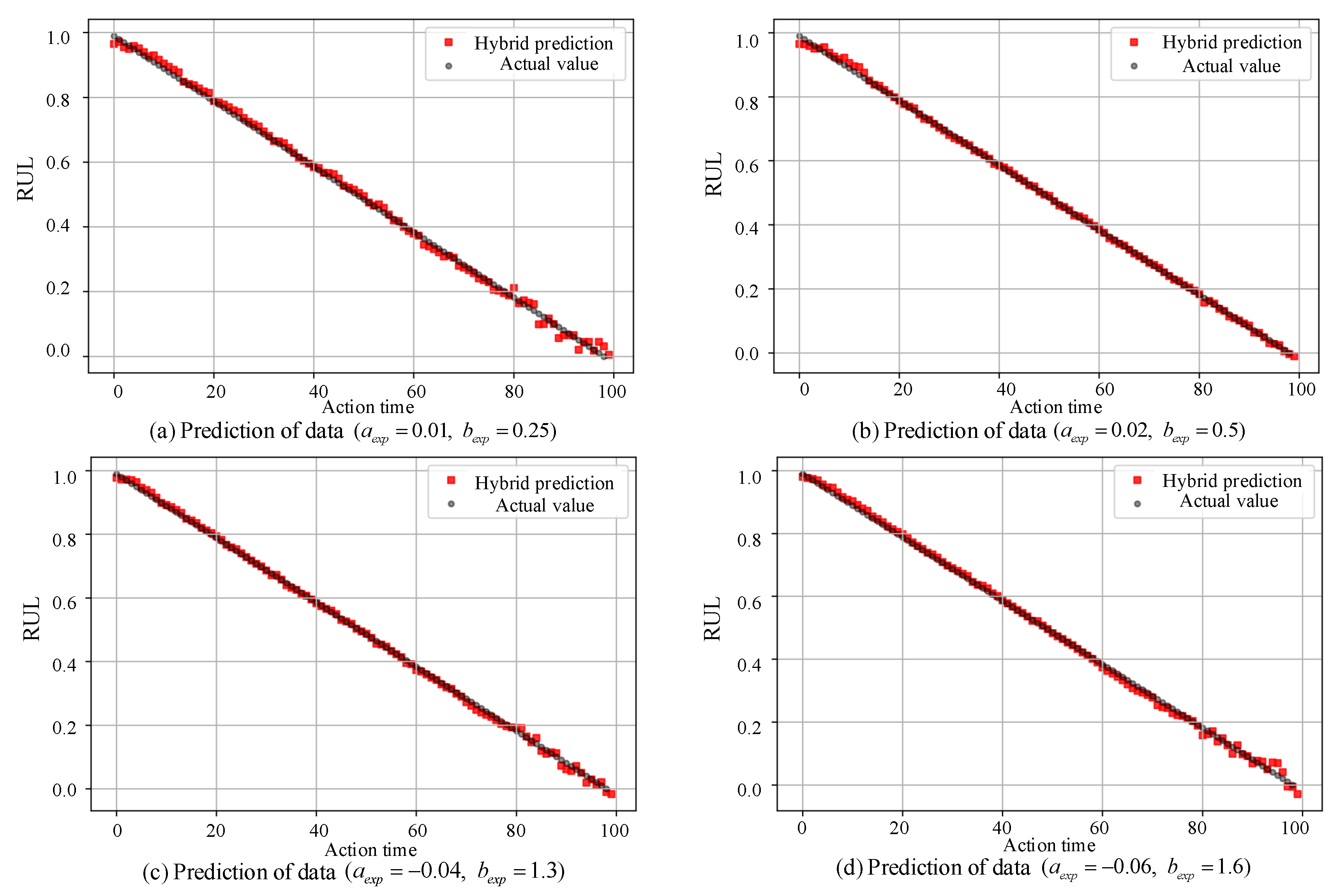
| (0.01, 0.25) | 1.58 | 1.93 | 2.94 | 3.45 | 3.62 | 3.88 | 4.22 | 4.60 | 4.80 | 4.84 | |
| 0.04 | 0.06 | 0.08 | 0.10 | 0.10 | 0.11 | 0.12 | 0.13 | 0.14 | 0.14 | ||
| (0.02, 0.5) | 4.91 | 4.99 | 5.36 | 6.86 | 12.21 | 12.52 | 17.20 | 17.84 | 18.44 | 19.98 | |
| 0.14 | 0.15 | 0.16 | 0.20 | 0.37 | 0.379 | 0.52 | 0.54 | 0.55 | 0.60 | ||
| (−0.04, 1.3) | 20.02 | 22.43 | 23.27 | 24.67 | 25.81 | 25.92 | 28.11 | 28.45 | 29.07 | 33.13 | |
| 0.60 | 0.67 | 0.70 | 0.74 | 0.78 | 0.79 | 0.85 | 0.86 | 0.88 | 1.00 | ||
| (−0.06, 1.6) | 33.80 | 33.84 | 33.91 | 34.04 | 34.08 | 35.59 | 35.86 | 37.51 | 37.68 | 39.32 | |
| 1.02 | 1.02 | 1.02 | 1.03 | 1.03 | 1.07 | 1.08 | 1.13 | 1.14 | 1.19 |
| Subset | Fault Type | Operation Mode | Training Scale | Testing Scale | Max-Lifespan | Selected Sensor |
|---|---|---|---|---|---|---|
| FD001 | 1 | 1 | 100 | 100 | 362 | 13 |
| FD002 | 1 | 6 | 260 | 259 | 378 | - |
| FD003 | 2 | 1 | 100 | 100 | 525 | 11 |
| FD004 | 2 | 6 | 249 | 248 | 543 | - |
| Methods | Metric | FD001 | FD002 | FD003 | FD004 |
|---|---|---|---|---|---|
| SVR | RMSE | 0.147 | 0.241 | 0.205 | 0.272 |
| Score | 1.139 | 3.874 | 1.757 | 4.461 | |
| CNN | RMSE | 0.132 | 0.234 | 0.193 | 0.243 |
| Score | 1.304 | 2.893 | 1.418 | 3.36 | |
| LSTM | RMSE | 0.149 | 0.223 | 0.215 | 0.231 |
| Score | 1.256 | 3.312 | 1.862 | 3.975 | |
| SAEs | RMSE | 0.145 | 0.259 | 0.233 | 0.294 |
| Score | 1.672 | 4.023 | 2.047 | 4.351 | |
| GBDT | RMSE | 0.124 | 0.213 | 0.218 | 0.302 |
| Score | 1.562 | 2.421 | 1.592 | 3.461 | |
| Proposed | RMSE | 0.119 | 0.172 | 0.184 | 0.217 |
| model | Score | 1.042 | 2.213 | 1.387 | 2.84 |
© 2020 by the authors. Licensee MDPI, Basel, Switzerland. This article is an open access article distributed under the terms and conditions of the Creative Commons Attribution (CC BY) license (http://creativecommons.org/licenses/by/4.0/).
Share and Cite
Peng, J.; Wang, S.; Gao, D.; Zhang, X.; Chen, B.; Cheng, Y.; Yang, Y.; Yu, W.; Huang, Z. A Hybrid Degradation Modeling and Prognostic Method for the Multi-Modal System. Appl. Sci. 2020, 10, 1378. https://doi.org/10.3390/app10041378
Peng J, Wang S, Gao D, Zhang X, Chen B, Cheng Y, Yang Y, Yu W, Huang Z. A Hybrid Degradation Modeling and Prognostic Method for the Multi-Modal System. Applied Sciences. 2020; 10(4):1378. https://doi.org/10.3390/app10041378
Chicago/Turabian StylePeng, Jun, Shengnan Wang, Dianzhu Gao, Xiaoyong Zhang, Bin Chen, Yijun Cheng, Yingze Yang, Wentao Yu, and Zhiwu Huang. 2020. "A Hybrid Degradation Modeling and Prognostic Method for the Multi-Modal System" Applied Sciences 10, no. 4: 1378. https://doi.org/10.3390/app10041378
APA StylePeng, J., Wang, S., Gao, D., Zhang, X., Chen, B., Cheng, Y., Yang, Y., Yu, W., & Huang, Z. (2020). A Hybrid Degradation Modeling and Prognostic Method for the Multi-Modal System. Applied Sciences, 10(4), 1378. https://doi.org/10.3390/app10041378