Spinal Cord Segmentation in Ultrasound Medical Imagery

Abstract

In this paper, we study and evaluate the task of semantic segmentation of the spinal cord in ultrasound medical imagery. This task is useful for neurosurgeons to analyze the spinal cord movement during and after the laminectomy surgical operation. Laminectomy is performed on patients that suffer from an abnormal pressure made on the spinal cord. The surgeon operates by cutting the bones of the laminae and the intervening ligaments to relieve this pressure. During the surgery, ultrasound waves can pass through the laminectomy area to give real-time exploitable images of the spinal cord. The surgeon uses them to confirm spinal cord decompression or, occasionally, to assess a tumor adjacent to the spinal cord. The Freely pulsating spinal cord is a sign of adequate decompression. To evaluate the semantic segmentation approaches chosen in this study, we constructed two datasets using images collected from 10 different patients performing the laminectomy surgery. We found that the best solution for this task is Fully Convolutional DenseNets if the spinal cord is already in the train set. If the spinal cord does not exist in the train set, U-Net is the best. We also studied the effect of integrating inside both models some deep learning components like Atrous Spatial Pyramid Pooling (ASPP) and Depthwise Separable Convolution (DSC). We added a post-processing step and detailed the configurations to set for both models.

1. Introduction

Two dimensional (2D) Ultrasound (US) is a standard modality in medical imaging [1,2,3,4,5]. It has several advantages. First, it does not have harmful effects on the human body. Second, it is relatively low cost compared with other modalities. Third, it provides real-time imaging during surgical operations [1,4,5]. The research community is actively concerned about the advancements made in the area of ultrasound imagery analysis [1,4,5,6,7]. This gives physicians the ability to get more information for image-guided intervention and surgery. One of the most tackled tasks in medical imaging analysis is the semantic segmentation of body organs and tissues [4]. This procedure makes a partitioning of the input image into separate regions. Every region has a particular clinical relevance [4].

On the other hand, Ultrasound imaging is challenging regards to the application of semantic segmentation algorithms. In fact, it is operator dependent and presents relatively fewer details compared to other modalities like Computerized Tomography scans (CT scan) or Magnetic Resonance Imaging (MRI) [4]. Furthermore, medically used ultra-sonographic waves do not pass through bones [5,6,7]. Even in the absence of bones, the depth penetration of the ultrasound waves depends on the acoustic impedance of the body organs. This makes an unclear representation of the organ boundaries [4].

The Spine is also called vertebral column, spinal column, or backbone. It is composed of several bones named vertebrae [2,3]. The basic functions of the spine are to protect the spinal cord and to maintain the body alignment. The spinal cord is a part of the central nervous system containing major nerve tracts [2,3]. It connects the brain to nerves throughout the body and helps to regulate body functions. The spinal cord descends out of the brain at the base of the skull through the spinal column until it ends at the second lumbar vertebrae. It is enclosed and protected inside the bones of the spinal column. It is approximately about 45 cm (18 inches) long with a varying width from 13 mm (0.5 inch) in the cervical and lumbar regions to 6.4 (0.25 inch) in the thoracic area [2]. Figure 1 shows a description of the human vertebrae from the anterior and the right lateral view.

Figure 2 demonstrated the location of the spinal cord inside the spinal canal of the vertebral column. We could realize the location of the lamina on the back part of the vertebra and behind the spinal cord.

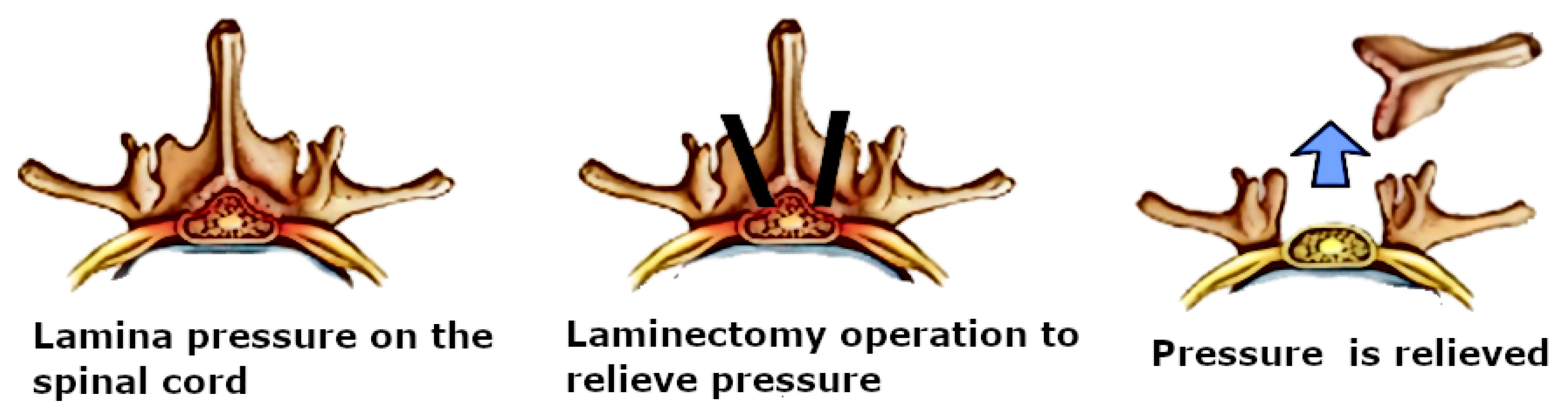
The laminectomy is a surgical operation performed by neurosurgeons and orthopedic surgeons to relieve compression on the spinal cord. This pressure may engender mild to severe back pain or difficulty in walking or in controlling limb functions. It can also have other symptoms that can interfere with daily life. The surgical procedure creates more space for the spinal cord and nerve roots to relieve abnormal pressure on the spinal cord by removing the laminae and the intervening ligaments [3]. Figure 3 shows the laminectomy surgery and the spinal cord.

In normal situations, the spinal cord could not be imaged using ultrasound imaging because ultrasonic waves do not pass well through bones [8]. In fact, the spinal cord is completely enclosed inside the bones of the spinal column. During laminectomy, ultrasonic waves can pass through the created bone defect to give real-time exploitable images of the spinal cord. Ultrasound imaging can demonstrate the spinal cord and the surrounding structures. This helps greatly to confirm the adequacy of the spinal cord decompression [8]. The ultrasound is also able to detect spinal cord pulsation and record it in a video format [8]. The created video can be saved for later use and analysis. It is believed that a decompressed spinal cord tends to have better pulsation. Spinal cord pulsation, however, is variable from one person to another [8]. Providing an automatic solution for detecting the exact boundaries of the spinal cord is helpful for automatic interpretation and analysis of spinal cord pulsation. This spinal cord pulsation values could be interpreted alongside the electrocardiogram (the electrical activity of the heart) to interpret if both signals are synchronized, or there is some latency to interpret [8].

But the great challenge here is the quality of the ultrasound image as boundaries could be obscured and some parts could be of foggy appearance [8]. This is due to the different attenuations applied to the sonographic waves while passing through the human body. This makes the automatic segmentation more difficult to achieve. But the service that gives this solution for neurosurgeons strengthens the interest for further examination to resolve this issue. Figure 4 gives a clear representation of how the spinal cord is represented in ultrasound imaging.

Since 2012 [9] deep learning based approaches have shown an attractive efficiency in object segmentation for multiple types of imaging (RGB imaging, aerial imaging, multi-spectral imaging etc.) [10,11,12,13,14]. This was a source of inspiration for the medical imaging community to move their interest towards a great adoption of these approaches for different medical imaging modalities (MRI, CT Scan, 2D Ultrasound, 3D Ultrasound etc.) [4].

Concerning the ultrasound medical segmentation, different works have been made in the detection of different parts of the body [4] (breast image segmentation, vessel image segmentation, heart image segmentation etc.). However, as demonstrated in Section 2, no one has treated the spinal cord image segmentation in 2D ultrasound medical imagery. In this study, we deduced, based on the current state of the art of image semantic segmentation, the best solution to adopt for our specific task. Our objectives in this paper were:

• Treating, for the first time, the problem of spinal cord segmentation in ultrasound imaging.
• Introducing, based on the state of the art in the area of image semantic segmentation, the best model for two case studies. The first case study is when the spinal cord is already in the train set of the model. The second case study is when the spinal cord does not belong to the train set of the model. We constructed a separate dataset for each scenario and selected the best model in each case study.
• Studying the integration of some successful deep learning components like ASPP (Atrous Spatial Pyramid Pooling) and DSC (Depthwise Separable Convolution) inside the selected models.
• Improving the performance of the chosen model by adding a post-processing step and selecting the right configuration setting for both models.

The rest of the paper is organized as follows: Section 2 was dedicated for a review about some related works that studied the spine anatomy in ultrasound imagery. Section 3 introduced the architecture of the selected models (FC-DenseNets and U-Net) and the deep learning components (ASPP and DSC) that we used for spinal cord ultrasound image segmentation. Section 4 discussed the experiments we made and the best approach to adopt for the different targeted scenarios.

2. Related Works

The analysis of ultrasound medical images of the spine was the subject of many studies in recent years. Ultrasound is a safe, radiation-free imaging modality that is easy to use by neurosurgeons compared to other medical imaging modalities. Pinter et al. [5] introduced a real-time method to automatically delineate the transverse processes parts of the vertebrae using ultrasound medical imagery. The method creates from the shadows cast by each transverse process a three-dimensional volume of the surface of the spine. Baum et al. [6] used the results of this study to build a step-wise method for identification of the visible landmarks in ultrasound to visualize a 3D model of the spine. Sass et al. [7] developed a method to make a navigated three-dimensional intraoperative ultrasound for spine surgery. They registered the patient automatically by using an intraoperative computed tomography before mapping it to a preoperative image data to get visualized navigation of the common parts of the spine. Hetherington et al. [15] developed a deep learning model named SLIDE to discriminate many parts of the spinal column using only 2d ultrasound with 88% cross-validation accuracy. The model acts in real-time (40 frames per second). Conversano et al. [16] developed a method for estimation of spine mineral density from ultrasound images. This method is useful for the diagnosis of osteoporosis. Zhou et al. [1] developed an automated measurement of the spine curvature from 3D Ultrasound Imaging. The method is useful for the diagnosis of scoliosis. Inklebarger et al. [17] developed a method to visualize transabdominal lumbar spine image using portable ultrasound. They specified a settings of machine configurations and probe selection to follow in order to obtain a profitable image. Karnik et al. [18] made a review of applications of the ultrasound imaging for the analysis of neonatal spine with emphasis on cases where it is the primary imaging modality to use. Di Pietro et al. [19] made a similar study on the examination of the neonatal and infant spine from the ultrasound. Ungi et al. [20] also made a review about applications of tracked ultrasound modality in navigation during spine Interventions. Chen et al. [21] made a pairwise registration of 2D ultrasound (US) and 3D computed tomography of the spine. The model is done using Convolutional Neural Network (CNN) before the refinement of the registration using an orientation code mutual information metric. Shajudeen et al. [22] developed a method for automatic segmentation of the spine bones surface in ultrasound images. The method can be extended to any bone surface presented in ultrasound images. Hurdle et al. [23] made a review about the use of ultrasound imagery for guidance in the diagnosis of many spinal pains.

From the above, we observed that a great number of studies had treated the use of ultrasound imagery in the diagnosis of clinical symptoms associated with the spine. Nevertheless, they are limited to the identification and segmentation of the bones of the spine. Up to our knowledge, no one treated the identification and segmentation of the spinal cord from ultrasound imaging. During laminectomy surgery, ultrasound images of the spinal cord could be visualized and analyzed. Surgeons usually refer to these images to study the effect of the laminectomy surgery and the spinal cord pulsation to confirm the adequacy of spinal cord decompression. Hence, we targeted this problem in this study and aim to provide an automatic solution for the segmentation of spinal cord using the recent advances in deep learning algorithms.

3. Proposed Method

This section gives an in-depth representation of the architecture of the models that have proven efficiency in our task of segmentation of the spinal cord inside ultrasound imagery. As U-Net and FC-DenseNets have proven efficiency in this mission, we will explain in detail the related concepts such as Convolutional Neural Network (CNN), U-net, DenseNets, and Fully Convolutional DenseNets. We will introduce later the Atrous Spatial Pyramid Pooling (ASPP) and the Depthwise Separable Convolution (DSC) and emphasize their usefulness in improving the performance of the chosen models.

3.1. CNN: Convolutional Neural Network

If we have data that contains N training samples ${\left\{(x_i,y_i)\right\}}_{i=1}^N$, where x represents the annotated input, y represents the label, Convolutional neural network (CNN) is able to construct a model F that maps the relationship between the input data x and the output data y. The CNN is built by stacking a series of layers that perform operations like convolution using a kernel function, non-linear activation, and max pooling. A training process of the model is used to give this built CNN model the set of parameters that best fits this mapping relationship with the minimal error. The training process includes five steps. The first step makes the initialization of the parameters and weights of CNN with random values. The second step is the forward propagation phase. During this step, a training sample $(x_i,y_i)$ is passed to the network, $x_i$ is transferred from the input layer to the output layer. Finally, we get the output $o_i$, which is formulated as:

$$\begin{array}{c}{o}_i=F_L(...)F_2\left(F_1\left(x_i{w}_1\right)w_2\right)...\left)w_L\right)\end{array},$$

(1)

L is the number of layers, $w_L$ is the weight vector of the Lth layer $F_L$.

The third step consists of estimating the loss function or the cost function, which is the function that calculates the error margin between the resulting output $o_i$ and the correct output value $y_i$. The fourth step will make the correction of the weight vector $w_1$, $w_2$, $w_3$, $w_L$ to minimize this loss function following this optimization problem:

$$\begin{array}{c}argmi{n}_{w_1,w_2,...,w_L}\frac{1}{N}\sum _{i=1}^{N}l(o_i,y_i),\end{array}$$

(2)

where l is the loss function. Usually, like here in our work, the cross-entropy loss function is used, as we made in the training phase of the model we adopted in this paper. In fact, we used a weighted version of cross-entropy to alleviate the imbalance between the class Spinal Cord and the class Other. To solve the numerical optimization problem, we use back-propagation and stochastic gradient descent methods. After this step, a more adequate set of parameters and weights is given to our model. In the fifth step, we will repeat the second, third, and fourth steps through all of the training data: ${\left\{(x_i,y_i)\right\}}_{i=1}^N$. Usually, this training will end by converging the loss function into a small value. This convergence is assured especially when we use a state of the art architecture like the architectures that we tested in this paper. Passing the full training data one time through the CNN network is named one epoch. Training CNNs usually involves running multiple epochs. Many techniques are used to make the cost function decrease faster. First, the Batch normalization technique [24] introduced in 2015 is becoming a state of the art method used, like we used here in our work, for normalizing the output of convolutional layers and fully connected layer before applying the non-linear activation function. This has a significant effect on making the loss function converge faster. Also, optimizers are also used to make the loss function converge faster. We used in our experiments the ADAM (Adaptive Moment Estimation) [25] introduced in 2015 as it is becoming a state of the art gradient descent optimizer.

3.2. Semantic Segmentation and U-Net Architecture

The semantic segmentation is the task of classifying every pixel inside an image into a meaningful category. In medical image analysis, semantic segmentation is a highly pertinent task. Computer-aided diagnosis relies heavily on the accurate segmentation of the organs and structures of interest in the captured medical image modalities (MRI, CT, Fluoroscopy, Ultrasound…). The success made by Convolutional Neural Networks had profoundly influenced the area of semantic segmentation. Many architectures had been proposed. Among the most used architectures in medical image segmentation, U-Net [26] is a state of the art model, Figure 5 represents the architecture of U-Net. U-Net model is an encoder-decoder architecture. The encoder is the contracting part on the left, and the decoder is the expansive path on the right side. The encoder part contains a series of 3 × 3 convolutions followed by a ReLU (Rectified Linear Unit) activation function. A 2 × 2 max-pooling operation is done after a series of consecutive convolutions for downsampling. The decoder part consists of upsampling the feature vector obtained at the end of the encoder part by a series of 2 × 2 up-convolutions to reconstruct the segmentation map at the size of the input image at the end. Between every up-convolutions operations, there are a series of 3 × 3 convolutions followed by ReLu similarly to the decoder part. Skip connections are added by copying the feature map of the encoder part with the correspondingly feature map of the decoder part. In the end, a sigmoid activation function is used to generate for each feature vector the desired class category. The network is trained end to end using back-propagation and stochastic gradient descent. As being discussed in the experimental part of this study, U-Net has proven efficiency where the spinal cord pattern is not previously learned by in the train set.

3.3. DenseNets and Fully Convolutional DenseNets

In 2017, Huang et al. [27] proposed the architecture of Densely Connected Convolutional Networks (or DenseNet) for image classification tasks. In this network, every layer is connected to every other layer in a feed-forward manner. Consequently, the input of every layer contains a concatenation of the feature maps of all preceding layers. Also, its own feature map is used as input in all subsequent layers. The network outperforms the state of the art networks on image classification problem, making it a strong feature extractor that can be used as a building block for other tasks like semantic segmentation. The network presents many advantages over its competitors. It mitigates the vanishing-gradient problem and reinforces feature propagation and reuse with smaller number of parameters. The architecture of the Dense block in Densenet is illustrated in Figure 6.

Formally, if we consider an image $x_0$ that passes through the DenseNet network that contains L layers. Each layer applies a transformation $F_l\left(\right)$ with l refers to the layer index. $F_l\left(\right)$ is composed of Convolution, Batch Normalization [24], ReLU [28] and Pooling [29]. If we set $x_l$ as the output of the lth layer, $x_l=F_l\left(x_{l-1}\right)$ for the traditional convolutional network. But in the dense block of the Densenet architecture, the lth layer of receives as input the feature map of all the preceding layers as expressed in Equation (3):

$$\begin{array}{c}{x}_l=F_l\left([x_0,x_1,...,x_{l-1}]\right),\end{array}$$

(3)

where $[x_0,x_1,...,x_{l-1}]$ is the concatenation of the feature maps generated in the preceding layers.

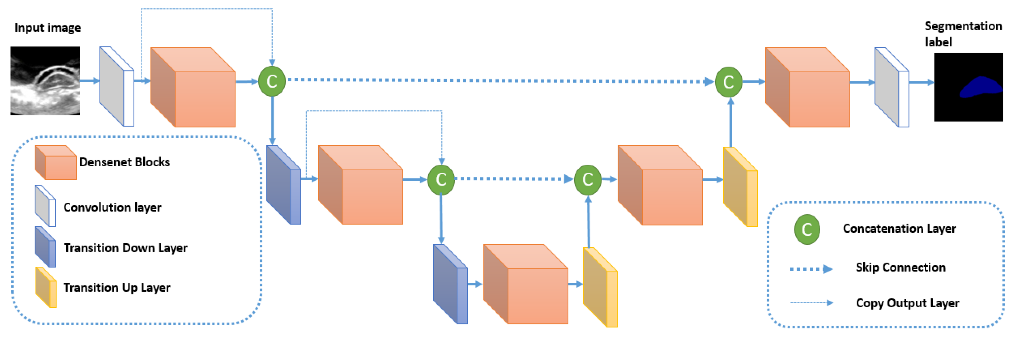
The architecture of Densenet is reused within the semantic segmentation context in the algorithm Fully Convolutional DenseNet (or FC-DenseNet) [30] by merging it inside an U-Net like model. The architecture of FC-Densenet is illustrated in Figure 7. The encoder path of FC-DenseNet corresponds to a DenseNet network that contains dense blocks separated by normal layers (Convolutions, Batch normalization, ReLu, and pooling). These normal layers form the transition down block that reduces the spatial resolution of each feature map using the pooling operation. The last layer of the encoder path is denoted as the bottleneck of the network. FC-Densenet adds a decoder path that aims to recover the original spatial resolution of the image. This decoder part contains Dense Blocks separated by Transition up blocks. The Dense blocks are similar to their corresponding Dense blocks in the encoder. The Transition Up block contains the up-sampling operations (transposed convolutions) necessary to compensate the down-sampling operations (pooling) in the encoder path. Similarly to U-Net, the Dense block of the two paths are connected by skip connections to guide the reconstruction of the input spatial resolution through the up-sampling part of the network. We can note that in the down-sampling path, the output of the dense block is concatenated to the output of the previous transition block to form the input for the next Transition down block. This operation is not used in the up-sampling path to reduce computations because already we have skip connection concatenated to every Dense Block input. The last layer in FC-Densenet is a 1 × 1 convolution followed by a softmax layer to generate for every pixel the per class distribution. The network is trained using cross-entropy loss calculated in a pixel-wise manner. The network can be trained from scratch without the need to train a feature extractor on external data as done in many state of the art segmentation algorithms. In our study, FC-DenseNet is proven to be the best tested algorithm in segmenting spinal cord when the pattern is already learned inside the training set. In this cases study, it outperforms U-Net.

3.4. Atrous Spatial Pyramid Pooling

As the shape and the size of objects inside the image may differ, the concept of image pyramid [31] had been introduced to improve segmentation precision. It consists on extracting features from different scales in a pyramid like approach before interpolating and merging them. But calculating the feature maps for every scale separately increases the size of the network and leads to heavy computations with risk of over-fitting. This is why a relevant method that combines the multiscale information in an efficient way is needed. Spatial pyramid pooling (SPP) [32] is proposed to treat this problem. SPP was first proposed to solve the issue of random input size of proposals in object detection [32]. SPP divides the randomly sized images into spatial bins before applying the pooling operation on every bin and concatenating them to obtain the fixed feature map size associated with this input image. Although its efficiency in capturing multi-scale features from the image, SPP is not well adapted to image segmentation because the pooling operations lose the pixel details needed for this task. Hence, we substituted the normal pooling layers in SPP by atrous convolutions with different sampling rates. Then, the extracted features from every sampling rate are merged to obtain the final feature vector. This method is called Atrous Spatial Pyramid Pooling (ASPP). The atrous convolution helps to have different receptive field for a convolution kernel by merely changing the sampling rate. This approach is the base of the state of the art model DeepLabv 3 plus [33], which is a segmentation model different in architecture from U-Net and FC-DenseNet. It is currently the best algorithm tested on PASCAL VOC dataset [34]. This is why we decided to study the effect of inserting an ASPP module inside the FC-DenseNet. Figure 8 illustrates the version of ASPP used in DeepLab v3 plus and in our experiments. Figure 9 shows the insertion of the ASPP module inside the DenseNet block to form an ASPP Dense Block. We will study the effect of this insertion inside the experimental part.

3.5. Depthwise Separable Convolution

Recently, MobileNet [35] had been introduced for efficient memory use and firstly designed for mobile and embedded devices. MobileNet is based on using Depth-wise Separable Convolutions (DSC), which have two benefits over traditional convolutions. First, they have a lower number of parameters to train as compared to standard convolutions. This makes the model more generalized and reduces overfitting. Second, they need a lesser number of computations for the training. DSC comprises of separating the standard convolution into two successive convolutions. The first convolution is performed separately over each channel of the input layer. Then, we apply a $1\times 1$ convolution to the output feature maps from the previous step to get the final output layer. Figure 10 illustrates the difference between standard convolution and depthwise separable convolution.

3.6. Postprocessing

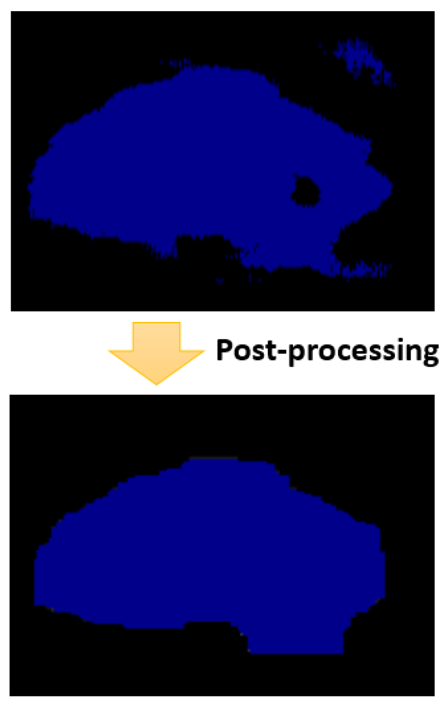
To raffinate the segmentation map generated by the semantic segmentation model, we applied a list of post-processing operations to improve the accuracy of segmentation. Figure 11 represents the status of a segmentation map of the spinal cord before and after the post-processing step.

The post-processing step is divided into four sub-steps. In every sub-step, we apply a different morphological operation on the segmentation map generated from the previous sub-step. The first sub-step is to remove small objects that the number of pixels is less than 1000. In fact, we always have in the ground truth one connected blob that corresponds to the spinal cord, with a number of pixels that is surely bigger than 1000 pixels. So, we removed small objects that contains a number of connected pixels less than 1000, and the degree of connectivity is set to 1. In fact, these removed objects correspond evidently for false-positive pixels. After that, we apply the second sub-step to the segmentation map generated from the first sub-step. This sub-step corresponds to removing small holes inside the spinal cord boundary. In fact, we are sure that the connected pixels corresponding to the spinal cord contain no holes. Hence, we removed these holes based on this property. Then, the third sub-step corresponds to apply a morphological closing using a square filter of size $4\times 4$ to make the boundary smooth and comparable to the boundary in real images. Then, we apply the last sub-step, which corresponds to a morphological opening using a square filter of size $4\times 4$. This intended to recover effects of the closing operation by filtering out the components that probably exceed the real spinal cord boundary. We will study in detail the effect of the post-processing step in the experimental part.

4. Experimental Results

This section will confirm the efficiency of the chosen approaches (FC-DenseNet and U-Net) by describing the implemented experiments and discussing the found results.

4.1. The Used Datasets and the Evaluation Metrics

4.1.1. The Used Datasets

To confirm the approaches adopted, we constructed 2 different datasets (Dataset-A and Dataset-B) based on ultrasound medical images collected from 10 patients during the laminectomy surgical operation. The surgeries were performed in King Saud University Medical City. All subjects gave their informed consent for inclusion before they participated in the study. The study was conducted in accordance with the Declaration of Helsinki, and the protocol was approved by the Ethics Committee of the Institutional Review Board of King Saud University Medical City (Project No. E-15-1602).

The first dataset is built to test the efficiency of the algorithm where the spinal cord exists within the training set. This dataset is formed by collecting significant images from the recorded ultrasound video captured during the laminectomy surgery. We mean by significant the existence of the spinal cord boundary in the images as sometimes the video contains many frames without clear spinal cord boundaries because the ultrasound probe was not set in the right place on top of the spine where the laminae were removed. Then, we cropped the zone containing the spinal cord into $256\times 256$ sized images. After that, we provided the pixel-wise manual segmentation of the image labeled by an expert and guided by two neurosurgeons working in the field of spine surgery. After that, we subdivided images for every patient into the train and the test sets following the rule of 80/20, which means putting 80 % of the labeled data inside the train set and 20% inside the test set.

Table 1. Composition of Dataset-A.

Patient ID	Total Number of Labeled Images	Images Put on the Train Set	Images Put on the Test Set
01	13	9	4
02	3	2	1
03	3	2	1
04	6	4	2
05	2	1	1
06	14	10	4
07	4	3	1
08	5	3	2
09	6	4	2
10	7	5	2
Total	63	43	20

provides details about Dataset-A used in validating the performance of the segmentation model on spinal cords already provided on the training set.

We built Dataset-B to validate model performance on spinal cords not previously provided in the train-set. It is formed by collecting ten different subsets. Every subset Dataset-$B^i$ is formed by putting all the images corresponding to the ith patient inside the test set and putting all the images of the other patients inside the train set. Then, measures will be calculated by averaging the results generated by the segmentation model on every Dataset-$B^i$. We aim by this method to test the generalization of the model on spinal cord patterns not provided in the train set in a cross-validation manner.

Table 2. Composition of Dataset-B (cross-validation).

Dataset	Patient IDs in the Train Set	Patient IDs in the Test Set	Number of Images in the Train Set	Number of Images in the Train Set
Dataset-B1	2…10	1	50	13
Dataset-B2	1,3…10	2	60	3
Dataset-B3	1,2,4…10	3	60	3
Dataset-B4	1…3,5…10	4	57	6
Dataset-B5	1…4,6…10	5	61	2
Dataset-B6	1…5,7…10	6	49	14
Dataset-B7	1…6,8…10	7	59	4
Dataset-B8	1…7,9,10	8	58	5
Dataset-B9	1…8,10	9	57	6
Dataset-B10	1…9	10	56	7
Dataset-B (cross validation)	1…10	1…10	63	63

gives us an idea about the composition of every Dataset-$B^i$ inside Dataset-B. We note that in every Dataset-$B^i$, the test set always contains spinal cord patterns not already learned by the model. This allows us to judge the ability of the model to be applied to new images taken for a new patient, which is the most probable scenario is real cases.

4.1.2. The Evaluation Metrics

To measure the efficiency of the semantic segmentation model, five metrics are used—Intersection over Union (IoU), Accuracy, Recall, Sensitivity, and Dice coefficient. The most important metric that allows to judge the global efficiency of the model is the IoU. IoU is calculated for every class independently before concluding the average IoU for all the classes. Giving two sets of data A and B, IoU is computed using the expression below:

$$IoU(A,B)=\frac{size(A\cap B)}{size(A\cup B)}.$$

(4)

Going deeper, the IoU is computed using four measures: $TP$ (True Positives), $TN$ (True Negatives), $FP$ (False Positives), and $FN$ (False Negatives). If we consider a semantic class C, $TP$ is the total of pixels of class C that was classified successfully as C by the algorithm. $TN$ is the number of pixels that don’t belong the class C and the algorithm did not associate them to C. $FP$ corresponds to the number of pixels that don’t belong to C and the algorithm associated them falsely to the class C. $FN$ is the count of pixels that belong to the class C and the algorithm was not able to classify them as C. Hence, IoU can be expressed explicitly as:

$$IoU=\frac{TP}{TP+FN+FP}.$$

(5)

Similarly, the other metrics are computed using the following expressions:

$$Accuracy=\frac{TP+TN}{TP+TN+FP+FN}$$

(6)

$$Precision=\frac{TP}{TP+FP}$$

(7)

$$Sensitivity=Recall=\frac{TP}{TP+FN}$$

(8)

$$DiceCoeff=F1Score=\frac{2\ast TP}{2\ast TP+FP+FN}.$$

(9)

4.2. Experiments on Dataset-A

4.2.1. Selection of the Best Performing Algorithm on Dataset-A

We began by evaluating the state of the art segmentation algorithms on Dataset-A. This aims to measure the ability of the algorithm to segment spinal cords that were already learned in the training set. We tested five state of the art algorithms. First, we tested Fully Convolutional DenseNets [30], we took the version FC-DenseNet103 as it is being considered as the best variation of FC-DenseNets [30]. We also tested Deeplab v3 plus [33], it is currently the state of the art model tested on Pascal VOC semantic segmentation dataset [34]. We tested PSPNet [36], which is currently the state of the art on Cityscapes semantic segmentation dataset [37]. We also tested two other state of the art algorithms, which are U-Net [26] and BiseNet [38]. To train these algorithms we used Semantic Segmentation Suite [39]. It is an open-source framework that contains implementations of some semantic segmentation algorithms in Tensorflow [40].

We made the training of the chosen algorithms on Dataset-A for 400 epochs. Figure 12 shows the measure of IoU on the test set of Dataset-A after every epoch of the training. It shows that FC-DenseNet103 and U-Net outperform clearly other algorithms. FC-DenseNet103 is slightly better than U-Net because the DenseNets block is more able to capture complex pattern provided in the data. Other algorithms are not capable to capture similarly the complexity of the data patterns inside small datasets like Dataset-A.

Table 3. Metrics measured for every segmentation algorithm.

Algorithm	IoU	Dice Score	Accuracy	Recall	Precision
FC-DenseNet103	0.946	0.989	0.989	0.989	0.989
UNet	0.944	0.988	0.988	0.988	0.988
BiSeNet	0.904	0.974	0.975	0.975	0.975
PSPNet	0.891	0.977	0.978	0.978	0.984
Deeplab v3+	0.879	0.976	0.975	0.975	0.978

shows the metrics measured of every one of the tested algorithms. The table shows that FC-DenseNet103 outperforms all other algorithms in all the metrics.

Figuress Figure 13 and Figure 14 show samples from each patient in Dataset-A. For each sample, we display the ground truth segmentation mask manually edited by an expert. Then, we show the predicted segmentation mask generated for every sample after training FC-DenseNet103 on Dataset-A. The figures show the high efficiency of the model on the task of spinal cord segmentation.

In order to improve more the accuracy, we picked out FC-DenseNet103 and applied a list of modifications. The modifications are detailed in the next sub-section

4.2.2. Modifications Applied to FC-DenseNet103

ASPP DenseBlock

In order to capture the multi-scales features inside the data, we replaced the DenseNet block in FC-DenseNet103 illustrated in Figure 6 by the ASPP-DenseNet block illustrated in Figure 9. We noted that the modification improves the convergence of the algorithm without improving the IoU.

Figure 15 shows the IoU change after every epoch of the training.

Table 4. Metrics measured before and after applying the ASPP block on FC-DenseNet103 network.

Algorithm	IoU	Dice Score	Accuracy	Recall	Precision
before	0.946	0.989	0.989	0.989	0.989
with ASPP	0.943	0.988	0.988	0.988	0.988

shows the metrics measured before and after applying the ASPP block on FC-DenseNet103.

The ASPP is a widely used concept in semantic segmentation. Some studies show an increase of efficiency when integrating it with FC-DenseNet in some tasks like breast tumor segmentation [41]. However, It does not help in improving the results in spinal cord segmentation. This is probably because the size of the spinal cord in the images has small variance and does not have multi-scale patterns to capture contrarily to the breast tumors [41], which differs largely in size.

Depthwise Separable Convolution

In order to reduce the size and the computations needed to train FC-DenseNet, we changed all the convolutional layers in the network by Depthwise Separable Convolutions (DSC). As expected, the operations reduce the size of the parameters without affecting the measured metrics. Only a slight decrease in convergence is noted as shown in Figure 16.

Table 5. Metrics measured before and after applying the Depthwise Separable Convolutions (DSC) on FC-DenseNet103 network.

Algorithm	IoU	Dice Score	Accuracy	Recall	Precision
before	0.946	0.989	0.989	0.989	0.989
with DSC	0.946	0.989	0.989	0.989	0.989

shows the metrics measured before and after applying the Depthwise Separable Convolutions (DSC) on FC-DenseNet103. On the other hand,

Table 6. Size of the model before and after applying the DSC on FC-DenseNet103 network.

Algorithm	Trainable Parameters	Size of the Model
before	9.26 MB	116.5 MB
with DSC	3.41 MB	50.4 MB

shows the reduction of size after the application of DSC.

Post-Processing

The morphological operations used in the post-processing step help to use geometric patterns existing in the data to improve accuracy after the application of the model. By applying the post-processing operations explained in Section III.F, an increase in the performance of segmentation is noted, as shown in Figure 17 and

Table 7. Metrics measured before and after applying the post-processing step on the FC-DenseNet103 network.

Algorithm	IoU	Dice Score	Accuracy	Recall	Precision
before	0.946	0.989	0.989	0.989	0.989
with post-processing	0.953	0.991	0.991	0.991	0.991

.

Set of Training Configurations

To more fine-tune the FC-DenseNet network, we concluded some configurations to use during the training of the network to improve the network efficiency:

• Data augmentation: we used vertical flip and horizontal flip transformation, brightness change of degree 20% and rotation transformation in the range of 20 degree.
• Weighted cross-entropy: We gave the weight 0.95 for the weight of the class spinal cord.
• ADAM optimizer: the best learning rate to use is 0.0001.

4.3. Experiments on Dataset-B

4.3.1. Selection of the Best Performing Algorithm on Dataset-B

After choosing the right algorithm and the right configuration to use on Dataset-A, we pass to Dataset-B. We aim by experiments on this dataset to test the generalization of the model and to segment successfully new spinal cords that are not in the training set. To select the best performing algorithm, we run the five segmentation model already tested on Dataset-A and trained it on every dataset Dataset-$B^i$ for 400 epochs. After that, we measure the average on all measures to judge fairly the algorithm that has performed well on new spinal cords. As shown in

Table 8. IoU measured for every algorithm on Dataset-B (cross-validation).

	U-Net	DenseNet-103	BiSeNet	PSPNet	DeepLab v3+
Dataset-B1	0.939	0.937	0.916	0.893	0.897
Dataset-B2	0.874	0.872	0.809	0.901	0.852
Dataset-B3	0.924	0.824	0.923	0.87	0.862
Dataset-B4	0.94	0.907	0.801	0.808	0.833
Dataset-B5	0.925	0.944	0.865	0.828	0.817
Dataset-B6	0.901	0.819	0.91	0.785	0.835
Dataset-B7	0.937	0.918	0.918	0.859	0.874
Dataset-B8	0.961	0.957	0.905	0.897	0.92
Dataset-B9	0.929	0.921	0.846	0.838	0.788
Dataset-B10	0.933	0.906	0.87	0.844	0.803
Dataset-B (cross validation)	0.9263	0.9005	0.8763	0.8523	0.8481

,

Table 9. Average Accuracy measured for every algorithm on Dataset-B (cross-validation).

	U-Net	FC-DenseNet-103	BiSeNet	PSPNet	Deeplab v3+
Dataset-B1	0.986	0.985	0.98	0.974	0.974
Dataset-B2	0.981	0.981	0.965	0.986	0.977
Dataset-B3	0.986	0.966	0.986	0.976	0.976
Dataset-B4	0.983	0.978	0.955	0.953	0.961
Dataset-B5	0.986	0.99	0.975	0.964	0.963
Dataset-B6	0.982	0.96	0.984	0.96	0.97
Dataset-B7	0.985	0.981	0.98	0.966	0.97
Dataset-B8	0.99	0.989	0.977	0.974	0.98
Dataset-B9	0.983	0.982	0.963	0.957	0.944
Dataset-B10	0.983	0.976	0.968	0.958	0.949
Dataset-B (cross validation)	0.9845	0.9788	0.9733	0.9668	0.9664

,

Table 10. Precision measured for every algorithm on Dataset-B (cross-validation).

	U-Net	FC-DenseNet-103	BiSeNet	PSPNet	Deeplab v3+
Dataset-B1	0.986	0.986	0.98	0.977	0.978
Dataset-B2	0.981	0.981	0.965	0.987	0.977
Dataset-B3	0.987	0.967	0.985	0.979	0.98
Dataset-B4	0.994	0.98	0.969	0.958	0.967
Dataset-B5	0.987	0.99	0.977	0.962	0.965
Dataset-B6	0.982	0.99	0.985	0.961	0.977
Dataset-B7	0.986	0.981	0.98	0.966	0.97
Dataset-B8	0.996	0.989	0.98	0.986	0.981
Dataset-B9	0.983	0.99	0.971	0.958	0.957
Dataset-B10	0.984	0.994	0.971	0.958	0.966
Dataset-B (cross validation)	0.9866	0.9848	0.9763	0.9692	0.9718

,

Table 11. Recall measured for every algorithm on Dataset-B (cross-validation).

	U-Net	FC-DenseNet-103	BiSeNet	PSPNet	Deeplab v3+
Dataset-B1	0.986	0.985	0.98	0.974	0.974
Dataset-B2	0.981	0.981	0.965	0.986	0.977
Dataset-B3	0.986	0.966	0.986	0.976	0.976
Dataset-B4	0.986	0.978	0.955	0.953	0.961
Dataset-B5	0.986	0.99	0.975	0.964	0.963
Dataset-B6	0.982	0.96	0.984	0.96	0.97
Dataset-B7	0.985	0.981	0.98	0.966	0.97
Dataset-B8	0.99	0.989	0.977	0.974	0.98
Dataset-B9	0.983	0.982	0.963	0.957	0.944
Dataset-B10	0.983	0.976	0.968	0.958	0.949
Dataset-B (cross validation)	0.9848	0.9788	0.9733	0.9668	0.9664

and

Table 12. Dice score (F1) measured for every algorithm on Dataset-B (cross-validation).

	U-Net	FC-DenseNet-103	BiSeNet	PSPNet	Deeplab v3+
Dataset-B1	0.986	0.985	0.98	0.975	0.974
Dataset-B2	0.98	0.98	0.962	0.986	0.977
Dataset-B3	0.987	0.966	0.985	0.977	0.977
Dataset-B4	0.986	0.979	0.959	0.955	0.963
Dataset-B5	0.987	0.99	0.976	0.962	0.964
Dataset-B6	0.981	0.957	0.984	0.96	0.972
Dataset-B7	0.986	0.981	0.98	0.966	0.97
Dataset-B8	0.99	0.989	0.978	0.975	0.98
Dataset-B9	0.983	0.981	0.965	0.956	0.943
Dataset-B10	0.983	0.976	0.969	0.957	0.952
Dataset-B (cross validation)	0.9849	0.9784	0.9738	0.9669	0.9672

, U-Net [26] outperforms clearly the state of the art algorithms in this task.

We deduce from the experiments that U-Net is able to learn complicated patterns from only a small sized data without memorizing the patterns existing in the train set. Hence, it will be the first choice algorithm to be adopted in the next steps of spinal cord analysis in ultrasound imagery. To improve moreover the performance of U-Net, we will cite in the next sub-section the right configuration to use. The integration of ASPP inside U-Net will not be tested following the conclusion we made on experiments made on Dataset-A. ASPP will not have a significant impact on accuracy because the patterns in our task do not have multiscale features to be learned. However, We will study the impact of the other modifications on U-Net (DSC, Post-processing, and set of training configurations).

4.3.2. Modifications Applied to U-Net

Depthwise Separable Convolution

To reduce the size and the computations needed for training U-Net, we substituted all the convolutional layers in the model by Depthwise Separable Convolution (DSC). We note that the size of the model was reduced by a factor of 4, and the global cross-validation accuracy was reduced by 0.0055, as shown in

Table 13. IoU measured on Dataset-B before and after applying the DSC on the U-Net network.

	U-Net (Before)	U-Net (After)
Dataset-B1	0.939	0.948
Dataset-B2	0.874	0.888
Dataset-B3	0.924	0.894
Dataset-B4	0.94	0.94
Dataset-B5	0.925	0.93
Dataset-B6	0.901	0.876
Dataset-B7	0.937	0.933
Dataset-B8	0.961	0.946
Dataset-B9	0.929	0.925
Dataset-B10	0.933	0.928
Dataset-B (cross validation)	0.9263	0.9208

and

Table 14. Size of the model before and after applying the DSC on the U-Net network.

	Trainable Parameters	Size of the Model
before	34.9 MB	420.7 MB
with DSC	8.8 MB	108.2 MB

.

Post-Processing and the Set of Training Configurations

These are the operations and the configuration to be used with U-Net to improve segmentation accuracy:

• Post-processing: This is an important step to implement especially when dealing with patterns not learned inside the train set. This will have a significant impact on reducing the False Positives and the False Negatives and increasing consequently the True Positives and the True Negatives.
• Data augmentation: we applied vertical flip and horizontal flip transformation, brightness change in range of 20%, and rotation transformation in the range of 20 degree.
• Weighted cross-entropy: We put the value 0.995 for the weight of the class spinal cord.
• ADAM optimizer: the best learning rate we tested in this task is 0.0001.

Table 15. IoU tested on Dataset-B using U-Net before and after using the chosen configurations.

	U-Net (Before)	U-Net (After)
Dataset-B1	0.939	0.941
Dataset-B2	0.874	0.899
Dataset-B3	0.924	0.953
Dataset-B4	0.94	0.936
Dataset-B5	0.925	0.936
Dataset-B6	0.901	0.928
Dataset-B7	0.937	0.95
Dataset-B8	0.961	0.969
Dataset-B9	0.929	0.917
Dataset-B10	0.933	0.947
Dataset-B (cross validation)	0.9263	0.9376

illustrates the effect of using these predefined configurations on the improvement of IoU on Dataset-B using U-Net.

We conclude that the post-processing step and the set of training configurations have a significant impact on improving the segmentation accuracy of U-Net.

5. Conclusions

In this study, we provided a solution to the problem of segmentation of the spinal cord in ultrasound imaging. This is done based on the state of the art algorithms existing in semantic segmentation. We constructed two datasets (Dataset-A and Dataset-B). Dataset-A tests the performance of the algorithm on spinal cord patterns already provided in the train set. Dataset-B tests the performance of the algorithm on new spinal cord patterns that are not provided in the train set in a cross-validation way. On Dataset-A, FC-DenseNet103 outperforms all the state of the art methods due to its capability to learn complex data patterns using the DenseNet Block. On Dataset-B, U-Net is the best due to its ability to learn complex patterns from a limited size of data without memorizing exactly the train set patterns. We found that the integration of the Atrous Spatial Pyramid Pooling module did not improve the performance of the model on our task. This is probably because the spinal cord in ultrasound images has a small variance in size and does not have multi-scale features to be captured using ASPP. We found that the Depthwise Separable Convolution (DSC) significantly reduces the size of the model, and the computations needed to train it without affecting the performance. We demonstrated that the post-processing step has a significant impact on improving the segmentation accuracy. We also concluded some configurations to be used during the training to fine-tune the model for best performance. Our work is the first step towards the automatic analysis of the spinal cord using intra-operative ultrasound medical imaging. The next task will be to automatically extract the pulsation curve of the spinal cord from the ultrasound video. This is useful to better analyze the movement of the spinal cord during the laminectomy operation and confirm the extent of decompression.

References

1. Zhou, G.Q.; Jiang, W.W.; Lai, K.L.; Zheng, Y.P. Automatic measurement of spine curvature on 3-D ultrasound volume projection image with phase features. IEEE Trans. Med Imaging 2017, 36, 1250–1262. [Google Scholar] [CrossRef] [PubMed]
2. Encyclopaedia Brittanica. Available online: https://www.britannica.com (accessed on 23 April 2019).
3. Virgina Spine Institute. Available online: https://www.spinemd.com/treatments/laminoplasty (accessed on 23 April 2019).
4. Litjens, G.; Kooi, T.; Bejnordi, B.E.; Setio, A.A.A.; Ciompi, F.; Ghafoorian, M.; van der Laak, J.A.; van Ginneken, B.; Sánchez, C.I. A survey on deep learning in medical image analysis. Med. Image Anal. 2017, 42, 60–88. [Google Scholar] [CrossRef] [PubMed] [Green Version]
5. Pinter, C.; Travers, B.; Baum, Z.; Kamali, S.; Ungi, T.; Lasso, A.; Church, B.; Fichtinger, G. Real-time transverse process detection in ultrasound. In Medical Imaging 2018: Image-Guided Procedures, Robotic Interventions, and Modeling; International Society for Optics and Photonics: San Diego, CA, USA, 2018; Volume 10576, p. 105760Y. [Google Scholar]
6. Baum, Z.; Church, B.; Lasso, A.; Ungi, T.; Schlenger, C.; Borschneck, D.P.; Mousavi, P.; Fichtinger, G. Step-wise identification of ultrasound-visible anatomical landmarks for 3D visualization of scoliotic spine. In Medical Imaging 2019: Image-Guided Procedures, Robotic Interventions, and Modeling; International Society for Optics and Photonics: San Diego, CA, USA, 2019; Volume 10951, p. 1095129. [Google Scholar]
7. Saß, B.; Bopp, M.; Nimsky, C.; Carl, B. Navigated 3-Dimensional Intraoperative Ultrasound for Spine Surgery. World Neurosurg. 2019, 131, e155–e169. [Google Scholar] [CrossRef] [PubMed]
8. Kimura, A.; Seichi, A.; Inoue, H.; Endo, T.; Sato, M.; Higashi, T.; Hoshino, Y. Ultrasonographic quantification of spinal cord and dural pulsations during cervical laminoplasty in patients with compressive myelopathy. Eur. Spine J. 2012, 21, 2450–2455. [Google Scholar] [CrossRef] [Green Version]
9. Krizhevsky, A.; Sutskever, I.; Hinton, G.E. Imagenet classification with deep convolutional neural networks. In Advances in Neural Information Processing Systems; MIT Press: Cambridge, MA, USA, 2012; pp. 1097–1105. [Google Scholar]
10. Benjdira, B.; Bazi, Y.; Koubaa, A.; Ouni, K. Unsupervised Domain Adaptation Using Generative Adversarial Networks for Semantic Segmentation of Aerial Images. Remote Sens. 2019, 11, 1369. [Google Scholar] [CrossRef] [Green Version]
11. Benjdira, B.; Khursheed, T.; Koubaa, A.; Ammar, A.; Ouni, K. Car Detection using Unmanned Aerial Vehicles: Comparison between Faster R-CNN and YOLOv3. In Proceedings of the 2019 1st International Conference on Unmanned Vehicle Systems-Oman (UVS), Muscat, Oman, 5–8 February 2019. [Google Scholar] [CrossRef] [Green Version]
12. Al Rahhal, M.M.; Bazi, Y.; Al Zuair, M.; Othman, E.; BenJdira, B. Convolutional neural networks for electrocardiogram classification. J. Med. Biol. Eng. 2018, 38, 1014–1025. [Google Scholar] [CrossRef]
13. Ammour, N.; Alhichri, H.; Bazi, Y.; Benjdira, B.; Alajlan, N.; Zuair, M. Deep learning approach for car detection in UAV imagery. Remote Sens. 2017, 9, 312. [Google Scholar] [CrossRef] [Green Version]
14. Benjdira, B.; Ammar, A.; Koubaa, A.; Ouni, K. Data-Efficient Domain Adaptation for Semantic Segmentation of Aerial Imagery Using Generative Adversarial Networks. Appl. Sci. 2020, 10, 1092. [Google Scholar] [CrossRef] [Green Version]
15. Hetherington, J.; Lessoway, V.; Gunka, V.; Abolmaesumi, P.; Rohling, R. SLIDE: Automatic spine level identification system using a deep convolutional neural network. Int. J. Comput. Assist. Radiol. Surg. 2017, 12, 1189–1198. [Google Scholar] [CrossRef]
16. Conversano, F.; Franchini, R.; Greco, A.; Soloperto, G.; Chiriacò, F.; Casciaro, E.; Aventaggiato, M.; Renna, M.D.; Pisani, P.; Di Paola, M.; et al. A novel ultrasound methodology for estimating spine mineral density. Ultrasound Med. Biol. 2015, 41, 281–300. [Google Scholar] [CrossRef]
17. Inklebarger, J.; Leddy, J.; Turner, A.; Abbas, B. Transabdominal Imaging of the Lumbar Spine with Portable Ultrasound. Int. J. Med Sci. Clin. Invent. 2018, 5, 3407–3412. [Google Scholar]
18. Karnik, A.S.; Karnik, A.; Joshi, A. Ultrasound examination of pediatric musculoskeletal diseases and neonatal spine. Indian J. Pediatr. 2016, 83, 565–577. [Google Scholar] [CrossRef] [PubMed]
19. Di Pietro, M.; Henningsen, C.; Hernanz-Schulman, M.; Paltiel, H.; Pruthi, S.; Rosenberg, H.; Cohen, H.; Phelps, A.; Silva, C.; Weinert, D.; et al. Ultrasound examination of the neonatal and infant spine. J. Ultrasound Med. 2016, 35, 9. [Google Scholar]
20. Ungi, T.; Lasso, A.; Fichtinger, G. Tracked ultrasound in navigated spine interventions. In Spinal Imaging and Image Analysis; Springer: New York, NY, USA, 2015; pp. 469–494. [Google Scholar]
21. Chen, F.; Wu, D.; Liao, H. Registration of CT and ultrasound images of the spine with neural network and orientation code mutual information. In Proceedings of the International Conference on Medical Imaging and Augmented Reality, Bern, Switzerland, 24–26 August 2016; Springer: New York, NY, USA, 2016; pp. 292–301. [Google Scholar]
22. Shajudeen, P.M.S.; Righetti, R. Spine surface detection from local phase-symmetry enhanced ridges in ultrasound images. Med. Phys. 2017, 44, 5755–5767. [Google Scholar] [CrossRef]
23. Hurdle, M.F.B. Ultrasound-guided spinal procedures for pain: A review. Phys. Med. Rehabil. Clin. 2016, 27, 673–686. [Google Scholar] [CrossRef]
24. Ioffe, S.; Szegedy, C. Batch Normalization: Accelerating Deep Network Training by Reducing Internal Covariate Shift. arXiv 2015, arXiv:1502.03167. [Google Scholar]
25. Kingma, D.P.; Ba, J. Adam: A Method for Stochastic Optimization. arXiv 2014, arXiv:1412.6980. [Google Scholar]
26. Ronneberger, O.; Fischer, P.; Brox, T. U-net: Convolutional networks for biomedical image segmentation. In Proceedings of the International Conference on Medical Image Computing and Computer-Assisted Intervention, Munich, Germany, 5–9 October 2015; Springer: New York, NY, USA, 2015; pp. 234–241. [Google Scholar]
27. Huang, G.; Liu, Z.; Maaten, L.v.d.; Weinberger, K.Q. Densely Connected Convolutional Networks. In Proceedings of the 2017 IEEE Conference on Computer Vision and Pattern Recognition (CVPR), Honolulu, HI, USA, 21–26 July 2017. [Google Scholar] [CrossRef] [Green Version]
28. Glorot, X.; Bordes, A.; Bengio, Y. Deep sparse rectifier neural networks. In Proceedings of the Fourteenth International Conference on Artificial Intelligence and Statistics, Fort Lauderdale, FL, USA, 11–13 April 2011; pp. 315–323. [Google Scholar]
29. LeCun, Y.; Bottou, L.; Bengio, Y.; Haffner, P. Gradient-based learning applied to document recognition. Proc. IEEE 1998, 86, 2278–2324. [Google Scholar] [CrossRef] [Green Version]
30. Jégou, S.; Drozdzal, M.; Vazquez, D.; Romero, A.; Bengio, Y. The one hundred layers tiramisu: Fully convolutional densenets for semantic segmentation. In Proceedings of the IEEE Conference on Computer Vision and Pattern Recognition Workshops, Honolulu, HI, USA, 21–26 July 2017; pp. 11–19. [Google Scholar]
31. Farabet, C.; Couprie, C.; Najman, L.; LeCun, Y. Learning hierarchical features for scene labeling. IEEE Trans. Pattern Anal. Mach. Intell. 2012, 35, 1915–1929. [Google Scholar] [CrossRef] [Green Version]
32. He, K.; Zhang, X.; Ren, S.; Sun, J. Spatial Pyramid Pooling in Deep Convolutional Networks for Visual Recognition. In Proceedings of the European Conference on Computer Vision, Zurich, Switzerland, 6–12 September 2014; Springer: Berlin, Germany, 2014; pp. 346–361, Lecture Notes in Computer Science. [Google Scholar] [CrossRef] [Green Version]
33. Chen, L.C.; Zhu, Y.; Papandreou, G.; Schroff, F.; Adam, H. Encoder-Decoder with Atrous Separable Convolution for Semantic Image Segmentation. In Proceedings of the European Conference on Computer Vision, Munich, Germany, 8–14 September 2018; Springer: Berlin, Germany, 2018; pp. 833–851, Lecture Notes in Computer Science. [Google Scholar] [CrossRef] [Green Version]
34. Semantic Segmentation on PASCAL Voc 2012 Dataset. Available online: https://paperswithcode.com/sota/semantic-segmentation-on-pascal-voc-2012 (accessed on 2 October 2019).
35. Howard, A.G.; Zhu, M.; Chen, B.; Kalenichenko, D.; Wang, W.; Weyand, T.; Andreetto, M.; Adam, H. MobileNets: Efficient Convolutional Neural Networks for Mobile Vision Applications. arXiv 2017, arXiv:1704.04861. [Google Scholar]
36. Zhao, H.; Shi, J.; Qi, X.; Wang, X.; Jia, J. Pyramid Scene Parsing Network. In Proceedings of the 2017 IEEE Conference on Computer Vision and Pattern Recognition (CVPR), Honolulu, HI, USA, 21–26 July 2017. [Google Scholar] [CrossRef] [Green Version]
37. Real-Time Semantic Segmentation on Cityscapes. Available online: https://paperswithcode.com/sota/real-time-semantic-segmentation-cityscap (accessed on 28 March 2019).
38. Yu, C.; Wang, J.; Peng, C.; Gao, C.; Yu, G.; Sang, N. BiSeNet: Bilateral Segmentation Network for Real-Time Semantic Segmentation. In Proceedings of the European Conference on Computer Vision, Munich, Germany, 8–14 September 2018; Springer: Berlin, Germany, 2018; pp. 334–349, Lecture Notes in Computer Science. [Google Scholar] [CrossRef] [Green Version]
39. Semantic Segmentation Suite. Available online: https://github.com/GeorgeSeif/Semantic-Segmentation-Suite (accessed on 28 March 2019).
40. Abadi, M.; Barham, P.; Chen, J.; Chen, Z.; Davis, A.; Dean, J.; Devin, M.; Ghemawat, S.; Irving, G.; Isard, M.; et al. TensorFlow: A system for large-scale machine learning. In Proceedings of the 12th USENIX Symposium on Operating Systems Design and Implementation (OSDI 16), Savannah, GA, USA, 2–4 November 2016; pp. 265–283. [Google Scholar]
41. Hai, J.; Qiao, K.; Chen, J.; Tan, H.; Xu, J.; Zeng, L.; Shi, D.; Yan, B. Fully convolutional densenet with multiscale context for automated breast tumor segmentation. J. Healthc. Eng. 2019, 2019, 8415485. [Google Scholar] [CrossRef] [PubMed] [Green Version]
Figure 1. Human vertebral column.
Applsci 10 01370 g001
Figure 2. The spinal cord inside the vertebral column.
Applsci 10 01370 g002
Figure 3. The laminectomy surgery.
Applsci 10 01370 g003
Figure 4. Ultrasound image of the spinal cord.
Applsci 10 01370 g004
Figure 5. Spinal Cord semantic segmentation using U-Net architecture.
Applsci 10 01370 g005
Figure 6. Dense block in DenseNet architecture
Applsci 10 01370 g006
Figure 7. Spinal Cord semantic segmentation using Fully convolutional DensenNets.
Applsci 10 01370 g007
Figure 8. Atrous Spatial Pyramid Pooling Module (ASPP).
Applsci 10 01370 g008
Figure 9. ASPP Dense Block.
Applsci 10 01370 g009
Figure 10. Depthwise Separable Convolution.
Applsci 10 01370 g010
Figure 11. Segmentation map of the spinal cord before and after the post-processing step.
Applsci 10 01370 g011
Figure 12. IoU after every epoch of the training.
Applsci 10 01370 g012
Figure 13. Samples from Dataset-A (patient 01 to patient 05), the ground truth and the predicted segmentation mask.
Applsci 10 01370 g013
Figure 14. Samples from Dataset-A (patient 06 to patient 10), the ground truth and the predicted segmentation mask.
Applsci 10 01370 g014
Figure 15. IoU after every epoch of the training before and after adding the ASPP block.
Applsci 10 01370 g015
Figure 16. Intersection of Union (IoU) before and after adding DSC on FC-DenseNet103 network
Applsci 10 01370 g016
Figure 17. IoU before and after adding the post-processing step.
Applsci 10 01370 g017