Bidirectional Sliding Window for Boundary Recognition of Pavement Construction Area Using GPS-RTK

Abstract

Unmanned pavement construction is of great significance in China, and the primary issue to be solved is how to identify the boundaries of the Pavement Construction Area (PCA). In this paper, we present a simple yet effective method, named the Bidirectional Sliding Window (BSW) method, for PCA boundary recognition. We first collected the latitude and longitude coordinates of the four vertices of straight quadrilaterals using the Global Positioning System—Real Time Kinematic (GPS-RTK) measurement principle for precise single-point positioning, analyzed single-point positioning accuracy, and determined the measurement error distribution models. Next, we took points at equal intervals along one straight line segment and two curved line segments with curvature radii of 70 m to 300 m, for simulation experiments. BSW was adopted to recognize the Possible Irrelevant Points (PIP) and Relevant Points (RP), which were used to identify PCA boundaries. Experiments show that when the proposed BSW algorithm is used and the single-point positioning accuracy is at the centimeter level, PCA boundary recognition for straight polygons reaches single-point positioning accuracy, and that for curved polygons reaches decimeter-level accuracy.

1. Introduction

In the field of robotic navigation, the road boundary recognition is mainly achieved using vision-based passive sensors [1,2] and lidar-based active sensors [3,4,5]. Vision-based sensors generally recognize road boundaries based on the physical and geometric characteristics of the roads, and lidar sensors generally determine the characteristics according to road boundary point cloud data to identify road boundaries. The literature shows that the fusion of the two algorithms can achieve a certain accuracy. However, the unconstructed road surface cannot provide sufficient physical, geometric features or point cloud data for identification by vision-based and lidar-based sensors.

Identification of the road boundary is also critical in the field of geographic information and plays a vital role in mapping, public management and road data updates. Many documents propose using GPS trajectories to extract and update road data, which generally involves using clustering [6,7,8], kernel density estimation [9,10], trajectory merging [11,12] and geometric modelling [13,14]. However, these methods extract road boundaries by analyzing and processing a large number of GPS trajectories, which are generally of meter-level accuracy [15]. According to actual construction requirements, the length of Pavement Construction Area (PCA) boundaries is generally only about 50 m and the width is only 10 to 20 m, but the positioning needs to be accurate to 1 decimeter. In addition, three types of construction joint—including stepped seams, miter seams and flat seams—are generally adopted during road construction, and both sides of the road may be straight or curved [16]. Figure 1 shows these six cases respectively.

To meet the needs of unmanned pavement construction, we generally design several paths parallel to one side of the road and the articulated road roller is required to track these planned paths in turn, as shown in Figure 2. Therefore, the designed construction boundaries, marked by the red curves in Figure 2, should accord with the curvature radius of the road. In general, the curvature radius of the road is 60 to 300 m. In this work, a curvature radius of 70 to 300 m was set for simulation experiments.

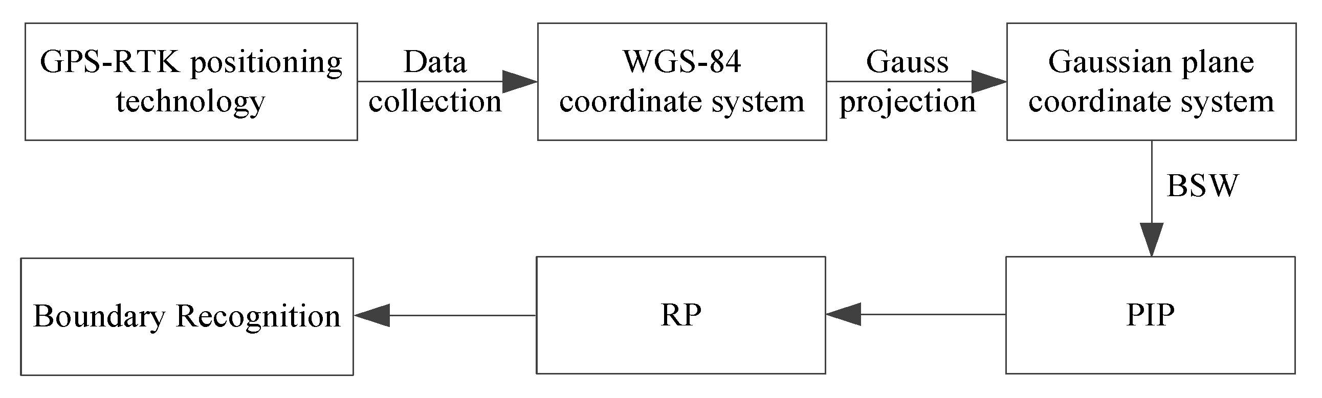
2. Boundary Recognition of Pavement Construction Area Using Global Positioning System—Real Time Kinematic (GPS-RTK)

In this section, GPS-RTK positioning technology is firstly introduced. Then, we describe how the latitude and longitude WGS-84 coordinate system data were extracted and converted into Gaussian plane coordinate format. Next, we describe how BSW was used to identify the Possible Irrelevant Points (PIP), and finally, we show how curve fitting with Relevant Points (RP) was applied to recognize the boundaries of the PCA. A flowchart describing PCA boundary recognition is shown in Figure 3.

2.1. GPS-RTK Positioning Technology

GPS provides single-point ten-meter-level positioning accuracy, and in order to obtain higher positioning accuracy, we usually use Differential GPS (DGPS) technology. This includes pseudorange differential positioning technology with decimeter-level positioning accuracy and RTK positioning technology with centimeter-level accuracy. The principle of these two different DGPS technologies is the same, that is, the base station determines errors in spatial correlation, the transmitting station broadcasts the error information and the mobile station receives both the GPS signal and the error information, based on which it quickly performs error correction. GPS-RTK was adopted for the work described in this paper, by which the carrier phase collected by the base station can be sent to the mobile station for precise single-point positioning.

2.2. WGS-84 Coordinate System to Gaussian Plane Coordinate System

To establish the relationship between the WGS-84 coordinate system (L,B) and the Gaussian plane coordinate system (x,y), the difference $l$ between geodetic longitude L and central meridian longitude $L_0$, and isometric latitude $q={\displaystyle {\int }_0^B\frac{M}{N\mathrm{cosB}}}\mathrm{dB}$ are introduced, and the relationship between ($l$,$q$) and (x,y) are established; that is:

$$\begin{array}{c}x=x(l,q)=m_0+m_2{l}^2+m_4{l}^4+\dots \\ y=y(l,q)=m_{1}l+m_3{l}^3+m_5{l}^5+\dots \end{array}$$

(1)

where $M=a(1-e^2)/{(1-e^2{\sin }^{2}B)}^{3/2}$ is the radius of curvature in the meridian and $N=a/{(1-e^2{\sin }^{2}B)}^{1/2}$ is the radius of curvature in the prime vertical, where $a=6399698.9018$ is the radius of the ellipsoid’s major axis and $e^2=0.0066943799013$ is the first eccentricity of the ellipsoid. The Gaussian projection satisfies the Cauchy-Riemann condition, as shown in Equation (2).

$$\begin{array}{c}\frac{\partial x}{\partial q}=\frac{\partial y}{\partial l}\\ \frac{\partial x}{\partial l}=-\frac{\partial y}{\partial q}\end{array}$$

(2)

Since the Gaussian projection does not change the length of the central meridian, the following equation exists:

$$x=m_0=X$$

(3)

where $X=6367558.49686*B/57.29577951308$ is the meridian arc length from equator to geodetic latitude $B$. The relationship between the WGS-84 coordinate system (L,B) and the Gaussian plane coordinate system (x,y) can be inferred from Equations (1)–(3), as shown in Equation (4):

$$\begin{array}{c}x=X+\frac{Nt}{2}{\cos }^{2}B{l}^2+\frac{Nt}{24}{\cos }^{4}B(5-t^2+9{\eta }^2+4{\eta }^4)l^4+\frac{Nt}{720}{\cos }^{6}B(61-58t^2+t^4)l^6\\ y=N\cos Bl+\frac{N}{6}{\cos }^{3}B(1-t^2+{\eta }^2)l^3+\frac{N}{120}{\cos }^{5}B(5-18t^2+t^4+14{\eta }^2-58{\eta }^2{t}^2)l^5\end{array}$$

(4)

where $t=\tan B$,${\eta }^2=e{}^{\prime 2}{\cos }^{2}B$ and $e{}^{\prime 2}=0.00673949674227$ is the second eccentricity of the ellipsoid.

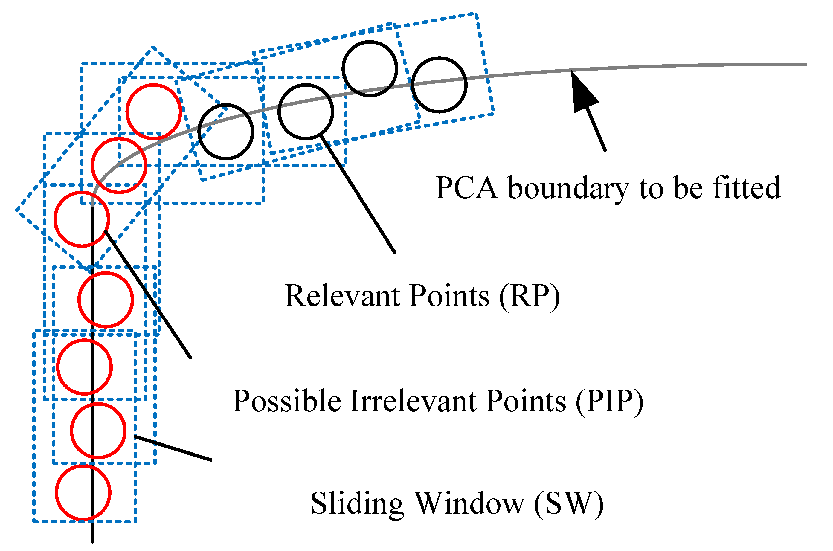
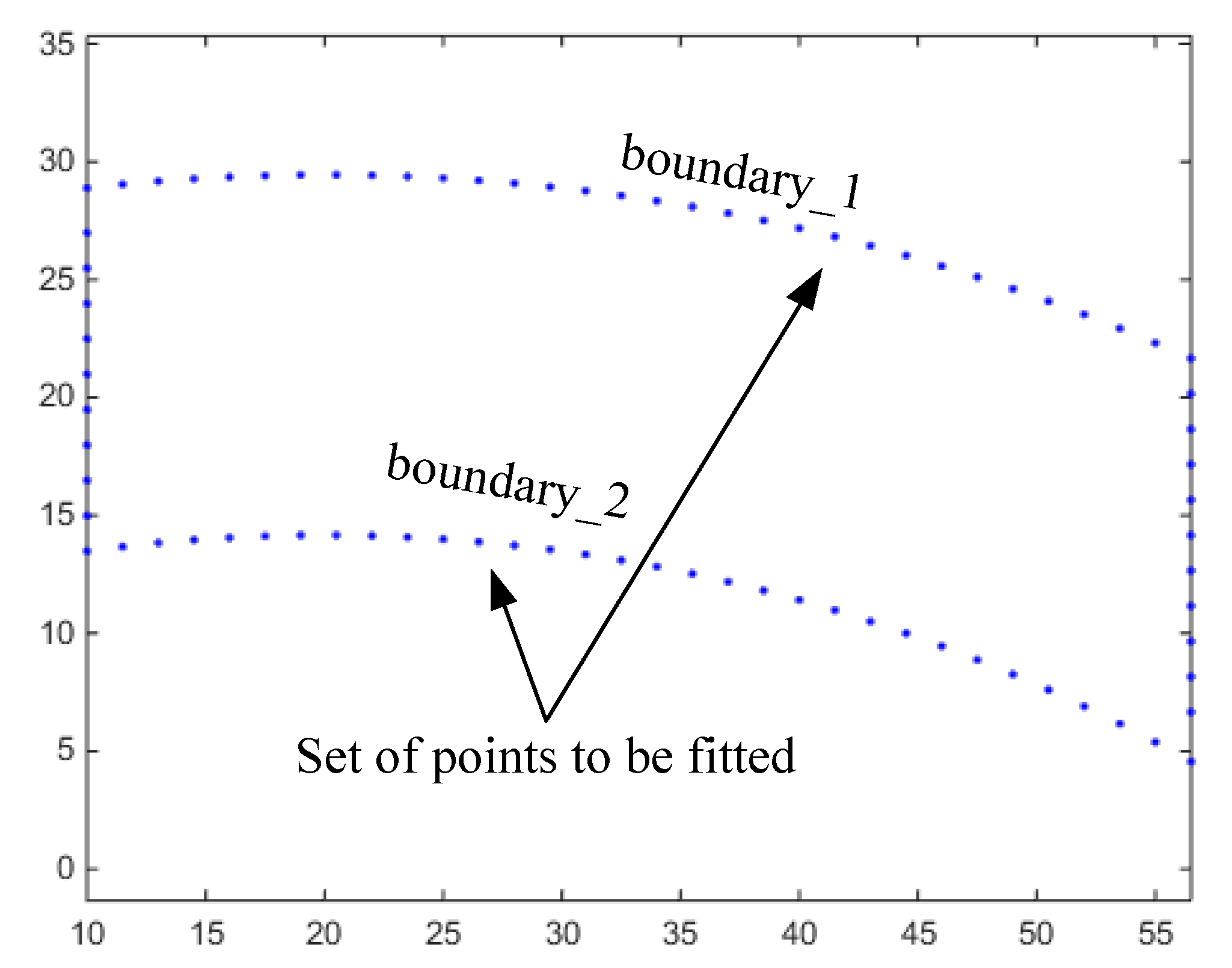
2.3. PCA Boundary Recognition with BSW

Sliding Window (SW) is a transmission control technology applied in the TCP (Transmission Control Protocol) and this algorithm only pays attention to the information in the window at each moment. As shown in Figure 4, the gray curve is the PCA boundary to be fitted. The SW with a window size of three to detect RP is indicated by the blue dotted boxes, and the red and black circles are the PIP and RP detected by the BSW algorithm, respectively.

Differently from the traditional SW algorithm, the proposed BSW algorithm selects the PIP by using the Sliding Window Clockwise (SWC) once and the Sliding Window Anticlockwise (SWA) once. As shown in Algorithm 1, the SWC and SWA flags are set to determine the proper window width and select PIP, and the RP data set is the DBD (abbreviation for DoubleBoundaryData mentioned in Algorithm 1) data set minus the PIP. In this paper, we call the proposed algorithm BSW due to the implementation of the SWC and SWA.

Algorithm 1: Boundary Recognition with BSW

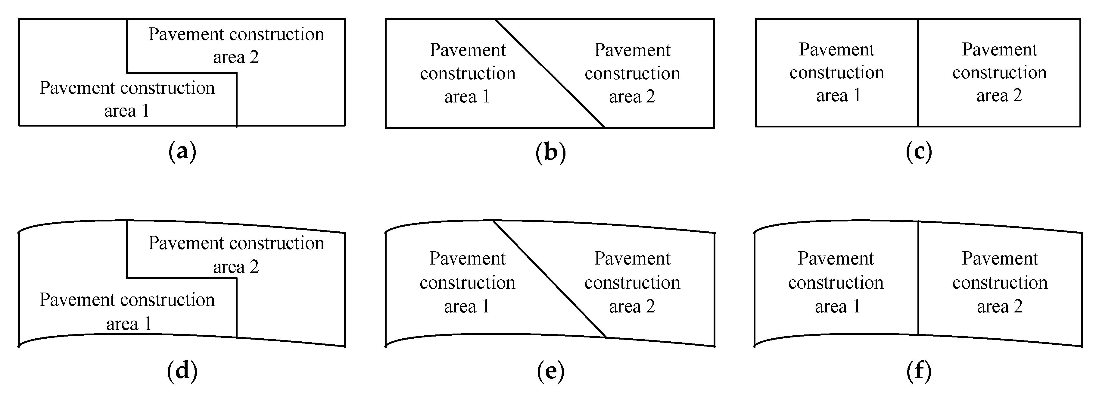
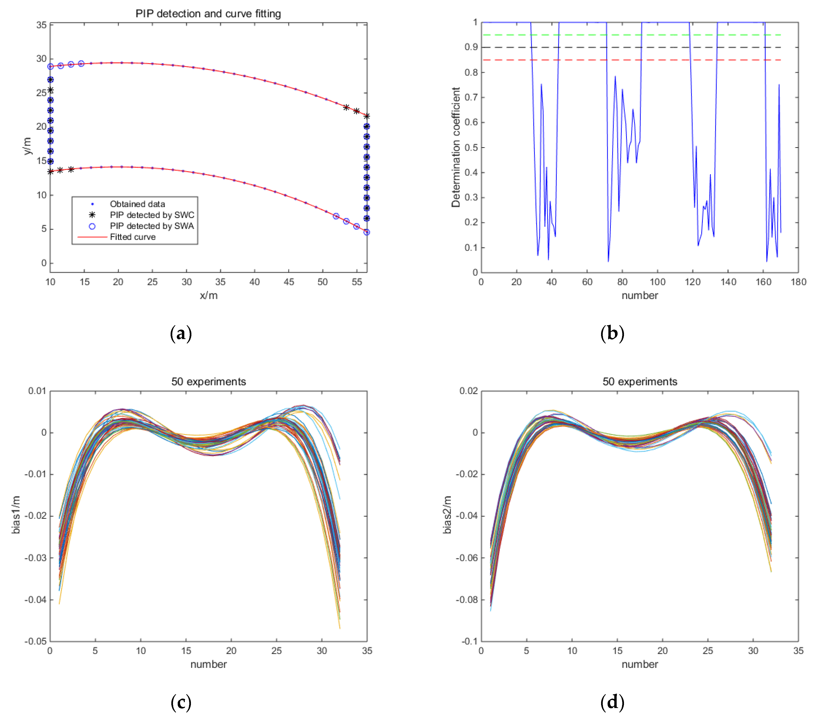
Input: WindowWidth Output: FittingError, WindowWidth Design a curved quadrilateral as shown in Figure 1f that meets the curvature constraints of the articulated road roller. Sample the curved quadrilateral and add the GPS-RTK measurement error distribution to simulate the acquired boundary data. To avoid data overflow in the experiment, double the boundary data and define variable DoubleBoundaryData as DBD. SWC ← 0, SWA ← 0, PIP ← {Ø}, RP ← {Ø}, While SWC == 0 do | PIPc ← {Ø} | for k ← 1 to K do | | Cofc ← SlidingWindowC (DBD, WindowWidth, k) | | if Cofc > 1 or Cofc <= 0 then | | └ WindowWidth ← WindowWidth + 1, break | | if Cofc < Thresholdc and Cofc > 0 then | | └ PIPc ← PIPc ∪ {DBD.k} | | Extract the set of more than two consecutive PIPc and mark them as C.a,C.b,…$\subset$ C | | if k == K and length(C) == 2 then └ └ └ SWC ← 1 While SWA == 0 do | PIPa ← {Ø} | for k ← 2K to K + 1 do | | Cofa ← SlidingWindowA (DBD, WindowWidth, k) | | if Cofa > 1 or Cofa <= 0 then | | └ WindowWidth ← WindowWidth + 1, break | | if Cofa < Thresholda and Cofa > 0 then | | └ PIPa ← PIPa ∪ {DBD.k} | | Extract the set of more than two consecutive PIPa and mark them as A.a,A.b,…$\subset$ A | | if k == K + 1 and length(A) == 2 then └ └ └ SWA ← 1 PIP ← PIPc ∪ PIPa RP ← DBD \ PIP FittingError ← BoundaryRecognition(RP)

3. Experiments

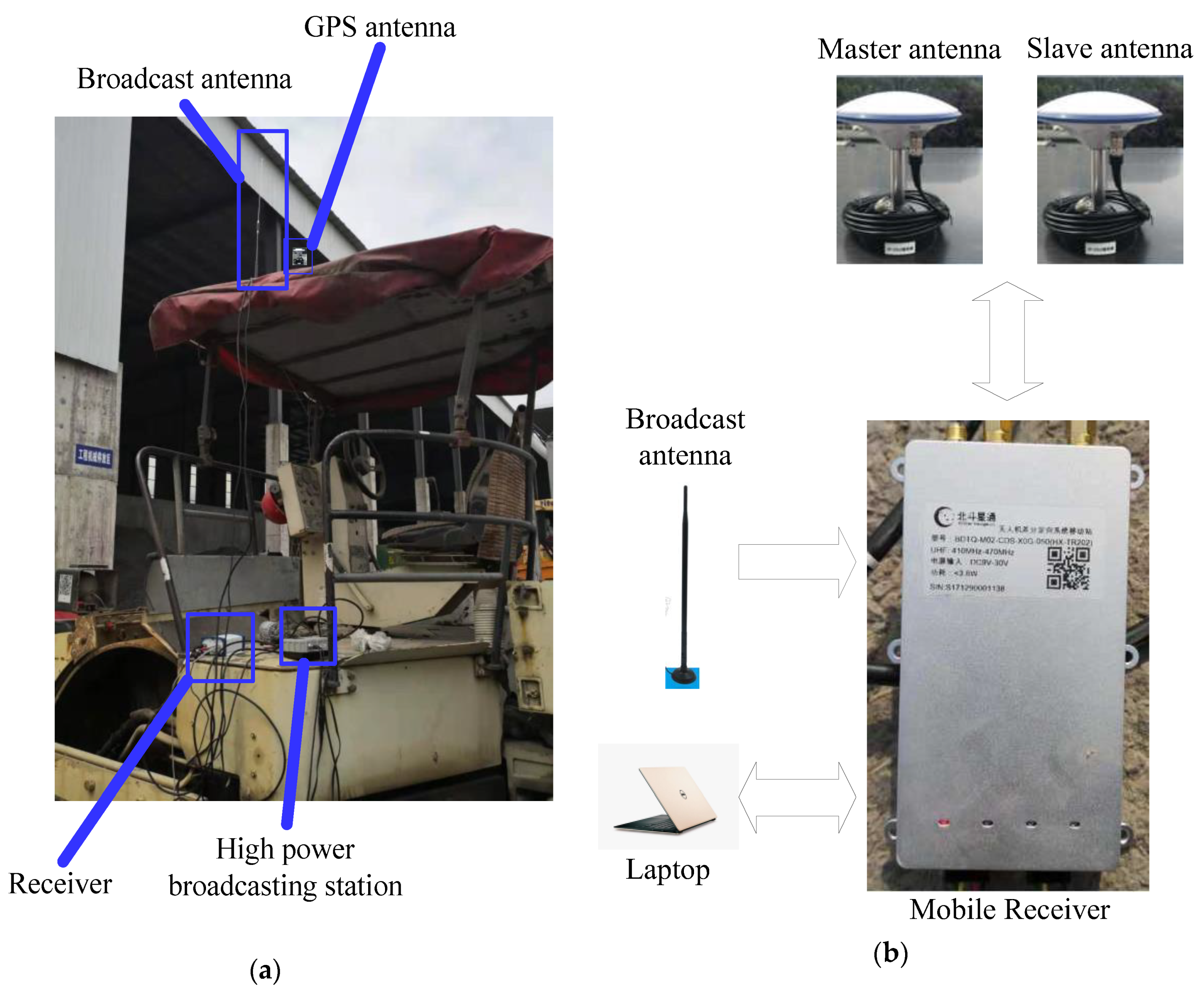
3.1. Experimental Platform

The experimental platform is shown in Figure 5 and it consisted of a base station, a transmitting station and a mobile station. The base station comprised a GPS antenna and a receiver, which was used to obtain spatial correlation error information, to be used by the mobile station to correct its observations. The transmitting station, composed of a broadcast station and a broadcast antenna, broadcasted the acquired error information. The mobile station received the GPS signal and the error information broadcast by the transmitting station, and used them to quickly perform error correction and improve single-point positioning accuracy. In this experiment, the carrier phase collected by the base station was sent to the mobile station for precise positioning. This technology is called Real-Time Kinematic (RTK), and it can achieve single-point centimeter-level positioning accuracy. In the field experiments, in order for good single-point positioning accuracy to be obtained, the base station needed to be free of obstruction in the space above the 10° elevation mask angle and it was necessary that there were no strong electromagnetic radiation sources nearby. The mobile station could not be too far away from the base station. In this experiment, the distance between the mobile station and the base station was less than 500 m.

3.2. Single-Point Positioning Accuracy and the Measurement Error Distribution Model

In order to recognize the quadrilateral PCA boundary with the proposed BSW algorithm in simulation, we needed to evaluate single-point positioning accuracy and determine the measurement error distribution model in the field experiments.

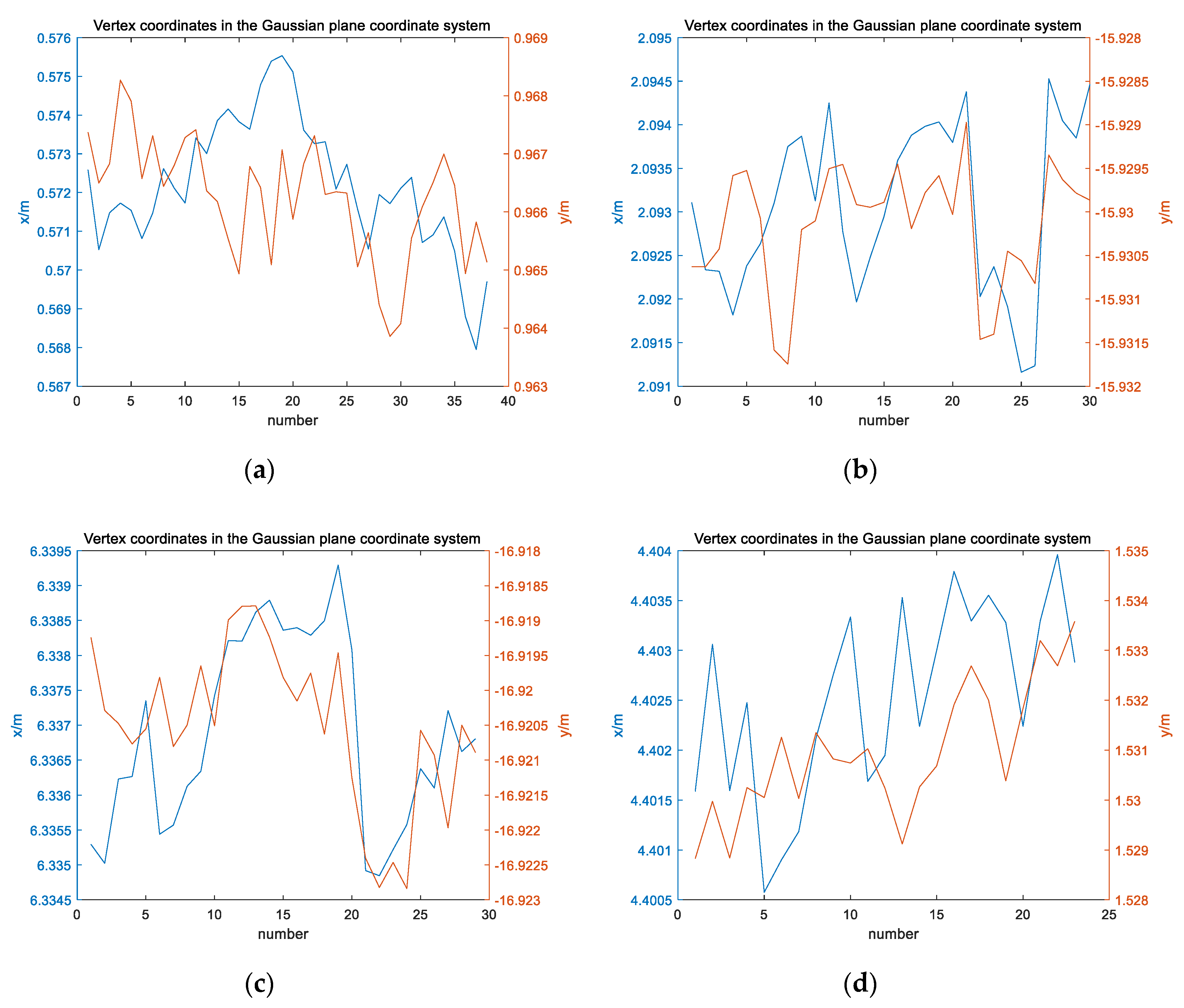
3.2.1. Single-Point Positioning Accuracy

We collected 20~40 data at each vertex of pavement construction area 1 in Figure Figure 1b. To enable the intuitive understanding of positioning accuracy, coordinate error of four vertices, shown in Figure Figure 6a(38 data), Figure 6b(30 data), Figure 6c(29 data), Figure 6d(23 data) respectively, were plotted at the meter scale in Gaussian plane format, where the average value of each vertex coordinate was taken as the true value around which the error distribution was calculated. In this way, we could determine whether the non-vertex coordinates were artificially collected by mistake.

Table 1. Covariance between abscissa and ordinates of the Gaussian plane coordinate system.

Cov(X1,Y1)	X1	Y1	Cov(X2,Y2)	X2	Y2
X1	2.93 × 10−6	1.71 × 10−7	X2	9.65 × 10−7	2.81 × 10−7
Y1	1.71 × 10−7	1.04 × 10−6	Y2	2.81 × 10−7	4.97 × 10−7
Cov(X3,Y3)	X3	Y3	Cov(X4,Y4)	X4	Y4
X3	1.86 × 10−6	8.94 × 10−7	X4	9.18 × 10−7	5.59 × 10−7
Y3	8.94 × 10−7	1.30 × 10−6	Y4	5.59 × 10−7	1.72 × 10−6

shows the covariance of the four vertices, and their values tend to zero, which means that the latitude and longitude of the four vertex coordinates are independent, and that the manually collected data could be further analyzed.

To further calculate the true values and confidence intervals for vertex coordinates, four vertices of the coordinates were plotted according to the double vertical axis system, as shown in Figure 7a–d, respectively. The horizontal axis represents the number of GPS data collected, the left vertical axis represents the x-axis of the Gaussian plane coordinate system in meters and the right vertical axis represents the y-axis of the Gaussian plane coordinate system in meters.

To ensure that the experimental equipment was kept in good condition during data acquisition, the T-test was adopted to determine whether the collected data met the single-point positioning accuracy requirements. As shown in

Table 2. Value range of coordinate parameters at the 95% confidence interval.

Coordinate Parameter	Value Range/m	Coordinate Parameter	Value Range/m
X1	(0.5717,0.5728)	Y1	(0.9659,0.9666)
X2	(2.0927,2.0934)	Y2	(−15.9304,−15.9299)
X3	(6.3364,6.3374)	Y3	(−16.9209,−16.9201)
X4	(4.4021,4.4029)	Y4	(1.5304,1.5315)

, the error of coordinate parameters was no more than 0.01 m at the 95% confidence interval. Therefore, the vertex coordinates in the Gaussian plane coordinate system can be finally determined, which are (0.57,0.97), (2.09,-15.93), (6.34,-16.92) and (4.40,1.53) respectively.

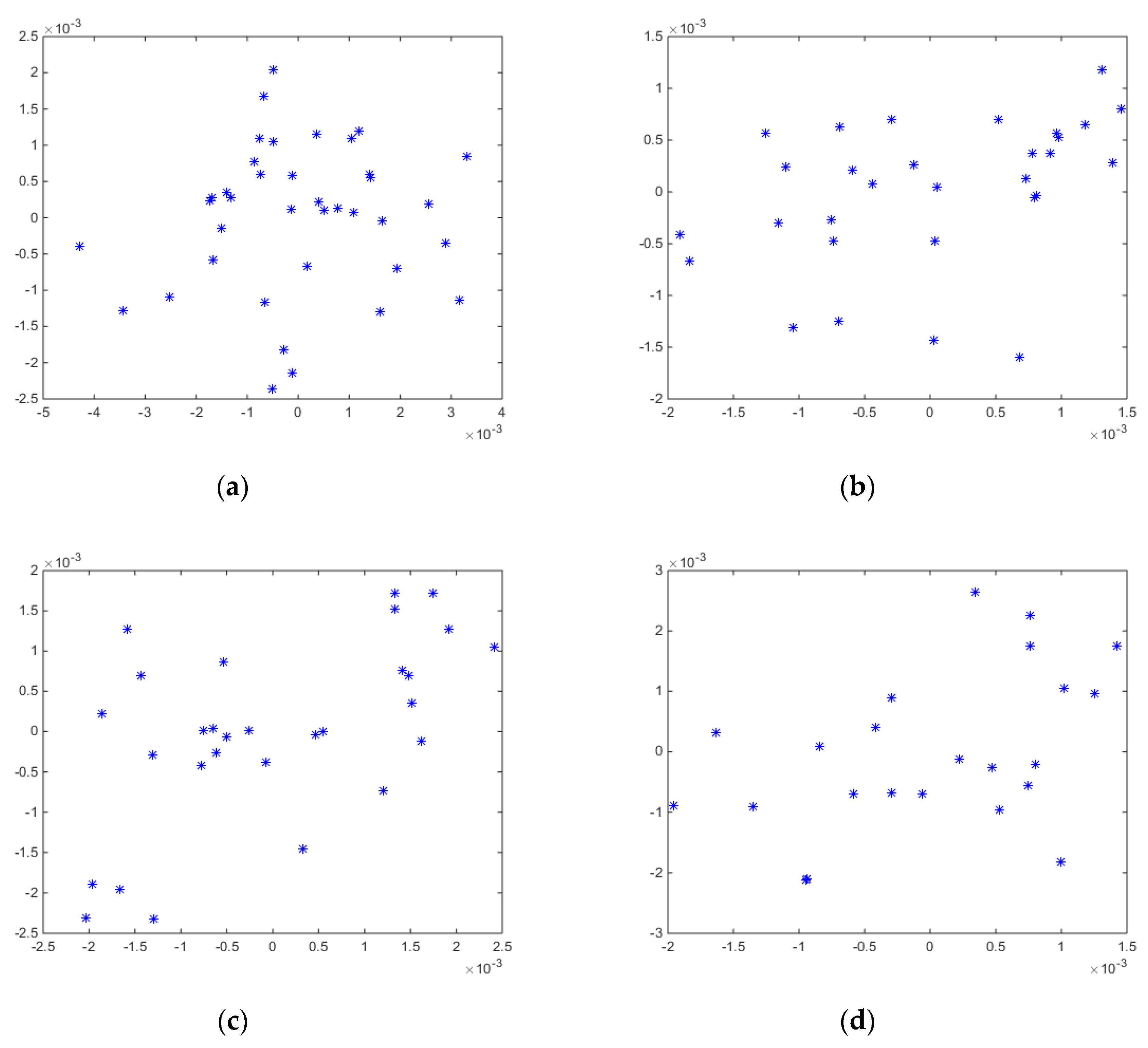
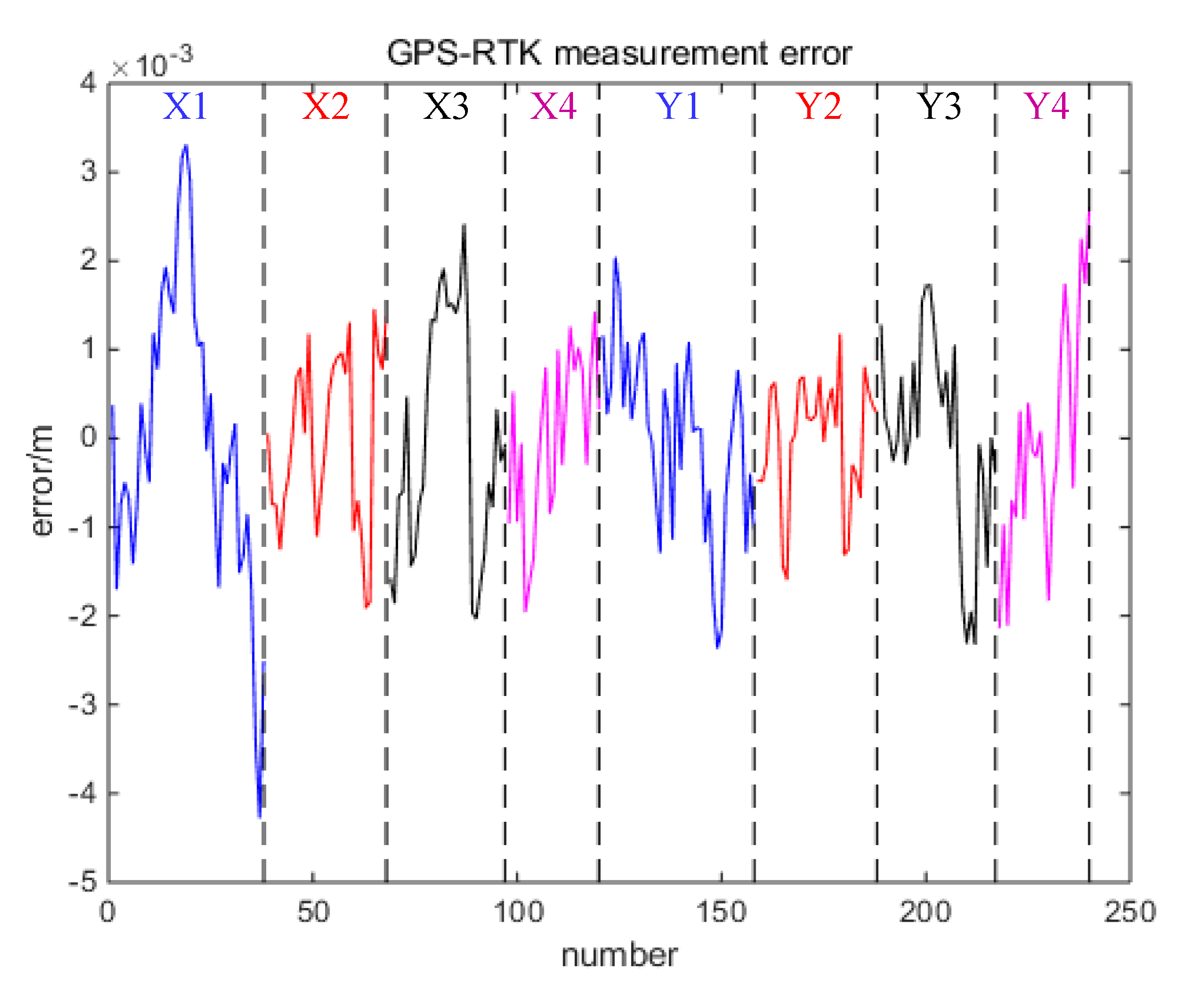
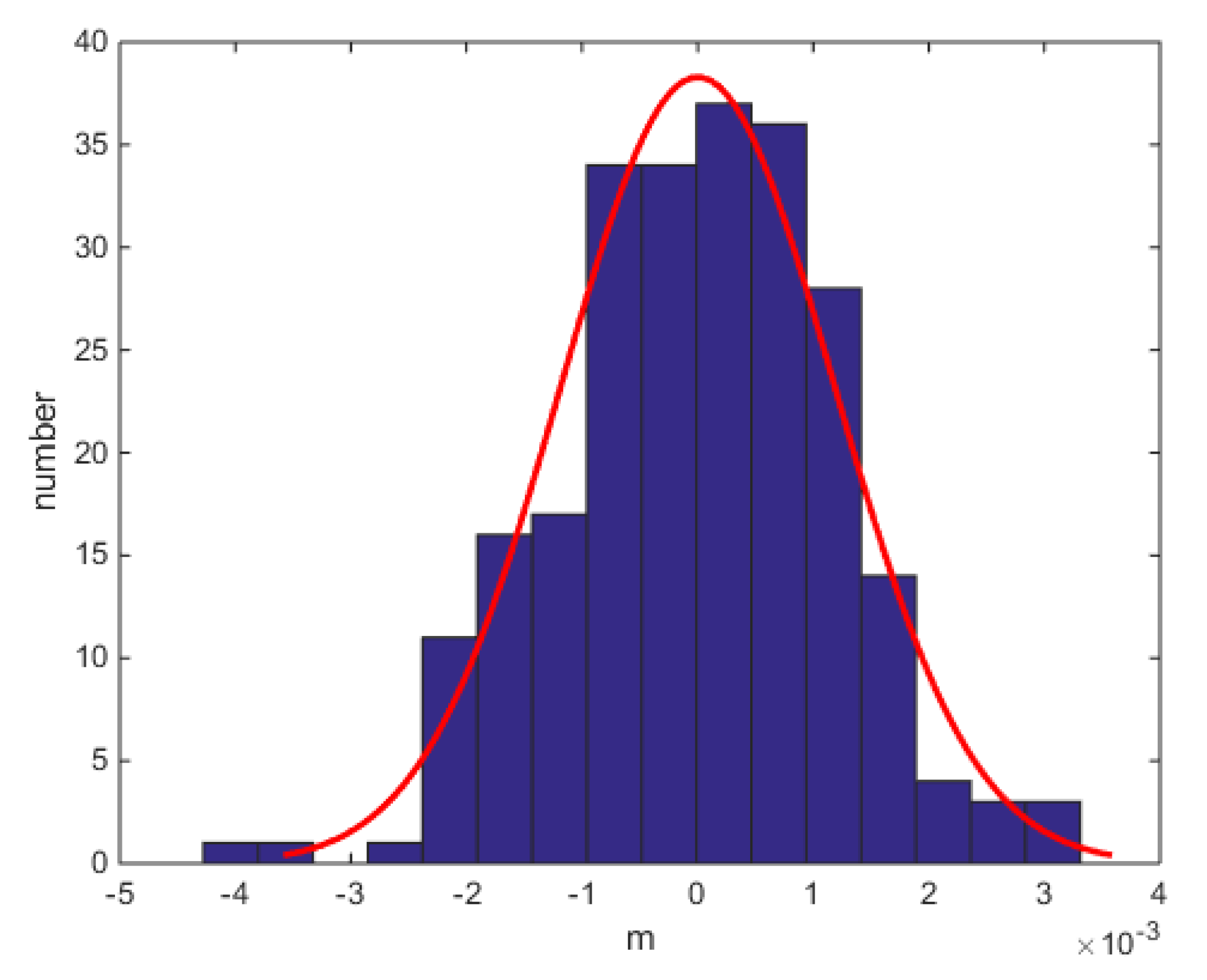
3.2.2. The GPS-RTK Measurement Error Distribution Model

To analyze the measurement error distribution model, we collected the GPS-RTK measurement errors of four vertex coordinates in the Gaussian plane coordinate system, as shown in Figure 8.

The Lilliefors test can check whether the sample data come from a normally distributed population. It is specifically implemented as follows: when the population mean and variance are unknown, they are replaced with the sample mean and variance, and then the Kolmogorov–Smirnov test is performed. In Matlab, the lillietest function can directly perform the Lilliefors test on the input vector, which was used to test the GPS-RTK measurement error, at the 0.05 significance level. The experimental results show that the data conform to a normal distribution, and their histogram and normal distribution curve are shown in Figure 9. The mean value of the random variable is −1.11 × 10⁻¹⁰, and the variance of the random variable is 1.41 × 10⁻⁶.

3.3. Recognition of Pavement Construction Area Boundary

The six types of polygon construction joints shown in Figure 1 can be divided into straight polygons (Figure 1a–c) and curved polygons (Figure 1d–f). This section introduces the method of identifying polygon boundaries from these two perspectives.

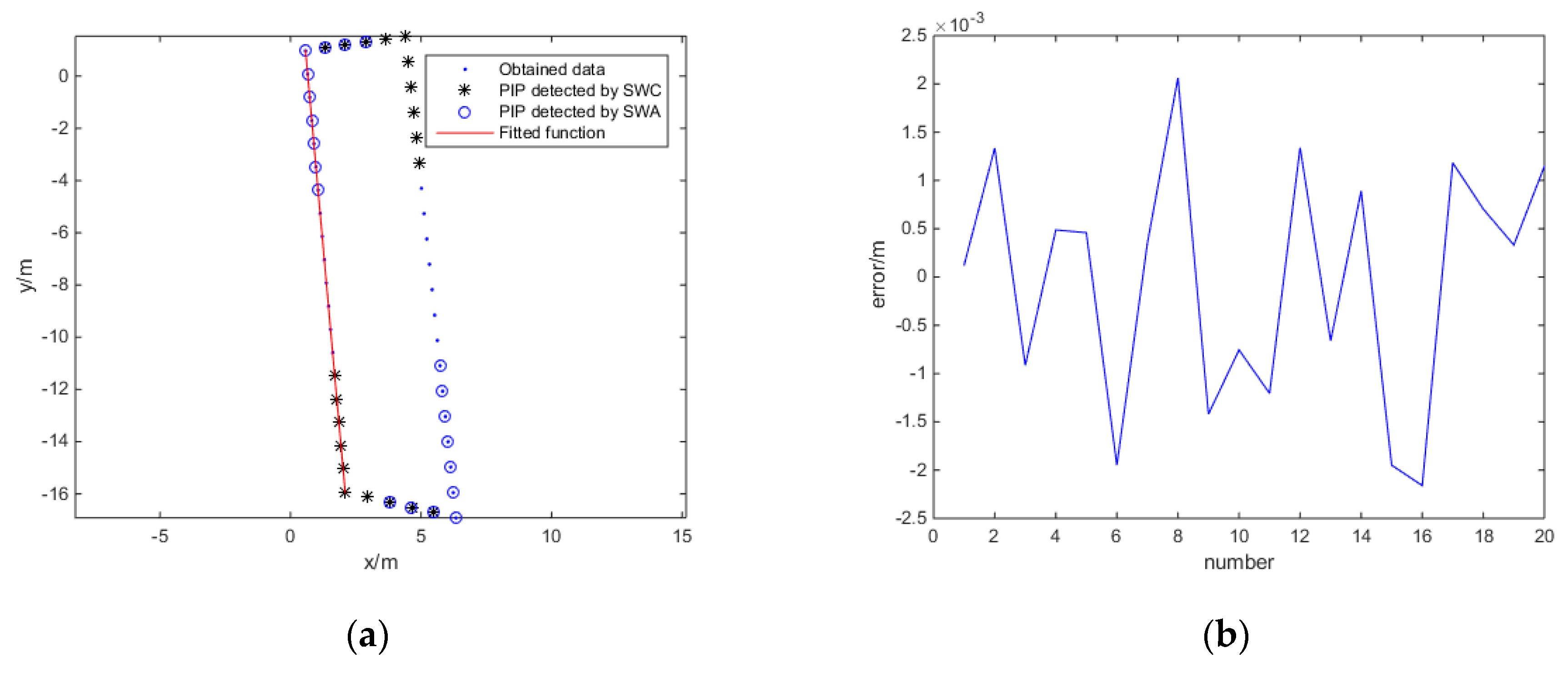
3.3.1. Recognition of Straight Polygon Pavement Construction Area Boundary

Three types of straight polygons PCA boundary shown in Figure 1a–c are all composed of straight line segments, so the recognition of the straight polygon PCA boundary can be regarded as identifying a straight line segment in the PCA boundary. Taking Figure 1b as an example, the GPS-RTK measurement errors mentioned in Section 3.2 were added and the proposed BSW was used for boundary recognition. As shown in Figure 10a, as long as there are more than two RP, the fitted function can be obtained regardless of the window size, and the accuracy of boundary recognition is high in terms of single-point positioning, as shown in Figure 10b.

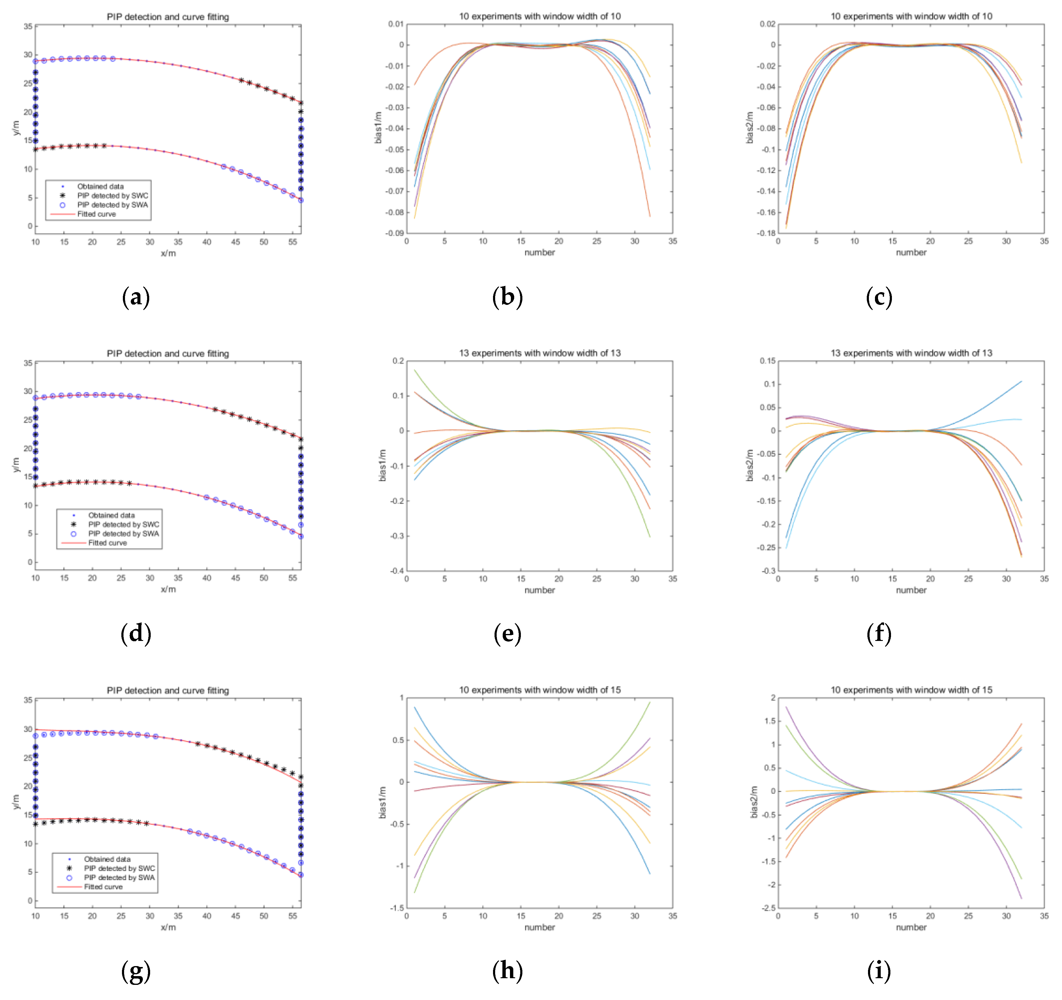
3.3.2. Recognition of Curved Polygon Pavement Construction Area Boundary

The three types of curved polygons PCA boundary shown in Figure 1d–f are all composed of straight line segments and curved line segments, and the method of identifying straight line segments was explained in Section 3.3.1. Identifying a curved line segment in the PCA boundary enables the recognition of that boundary. We designed two curves along the road with curvature radii of 70 to 300 m as mentioned in Section 1 and then added the GPS-RTK measurement errors as mentioned in Section 3.2. Then, we sampled the two curves to simulate the data acquired by GPS-RTK, as shown in Figure 11.

Figure 12 shows the PIP detected by the BSW algorithm and the fitting error across 10 experiments with window widths of 10, 13 and 15 respectively. Figure 12a,d,g show PIP detection and curve fitting. Specifically, blue dots indicate the obtained data, black stars and blue circles represent PIP detected by SWC and SWA respectively, and the red curve is the fitted curve. Figure 12b,e,h and Figure 12c,f,i indicate the deviation between the data points on the two curves to be fitted and the actual deviation under different window sizes. From Figure 12, it can be seen that the larger the window size, the more PIP, and the larger the error of the fitted curve on both sides. Therefore, the size of the sliding window should be set as narrow as is possible whilst allowing the algorithm to effectively detect the PIP.

However, when the window was too small, the algorithm could recognize some of the PIP, as is shown in Figure 13a. Figure 13b shows the determination coefficient of the sliding window at each point and we can see that the small amplitude fluctuation of the determination coefficients greatly affected PIP identification; that is, PIP was extremely sensitive to fluctuations in the determination coefficients, which must be avoided. Therefore, it is extremely important to set the SW at an appropriate width.

We used Algorithm 1, mentioned above, for experimental verification, as shown in Figure 14a,b. Although there were some misdetected PIP, PIP detection was no longer sensitive to fluctuations of determination coefficients. Due to the randomness of the measurement error, we conducted 50 experiments and plotted the bias between the acquired data and the fitted data. As shown in Figure 14c,d, the RP fitting effect over the middle section of the curve was good, almost reaching GPS-RTK single-point positioning accuracy; the PIP fitting effect of the two sides of the curve was slightly worse, but accuracy was at worst to the 0.1 m level.

3.4. Discussion of Results

This part discusses the results mentioned in the first three parts of this section. In the first part, we gave a brief introduction to the experimental platform. In the second part, we described the collection of the latitude and longitude coordinates of the four vertices of the straight quadrilateral PCA boundary, the analysis of the single-point positioning accuracy and the determination of the GPS-RTK measurement error distribution model. In the third part, we described how we took points at equal intervals across one straight line segment and two curved line segments with curvature radii of 70 to 300 m for simulation experiments, explored the effect of window width and determination coefficient on the experiments, and finally achieved good experimental results by the proposed BSW algorithm in both straight and curved polygons.

4. Conclusions

The mainstream boundary recognition algorithms are generally based on the physical and geometric characteristics of roads, or the processing of a large number of GPS trajectories. Differently from these existing algorithms, the work reported in this paper focused on solving the problem of identifying PCA boundaries without any physical and geometric characteristics or large amounts of GPS data. To this end, we proposed the BSW method for PCA boundary recognition, using GPS-RTK. Our simulation experiments showed that when the proposed BSW algorithm was used and the single-point positioning accuracy was at the centimeter level, PCA boundary recognition for straight polygons reached single-point positioning accuracy, and PCA boundary recognition for curved polygons reached decimeter-level accuracy.

In future research, we will use GPS equipment to obtain pavement construction boundary data, adopt the algorithm proposed in this paper to find the pavement construction boundary function, and plan the paths that the articulated road roller should track.

References

1. Yang, B.; Xu, X.; Li, J.; Zhang, H. Landmark generation in visual place recognition using multi-scale sliding window for robotics. Appl. Sci. 2019, 9, 3146. [Google Scholar] [CrossRef] [Green Version]
2. Zhang, Y.; Wang, H.; Zhou, H.; Deng, P. A mixture model for image boundary detection fusion. IEICE Trans. Inf. Syst. 2018, E101D, 1159–1166. [Google Scholar] [CrossRef] [Green Version]
3. Kwak, K.; Huber, D.F.; Chae, J.; Kanade, T. Boundary detection based on supervised learning. In Proceedings of the 2010 IEEE International Conference on Robotics and Automation, Anchorage, AK, USA, 3–7 May 2010; pp. 3939–3945. [Google Scholar]
4. Li, X.; Wang, D.; Ao, H.; Belaroussi, R.; Gruyer, D. Fast 3D semantic mapping in road scenes. Appl. Sci. 2019, 9, 631. [Google Scholar] [CrossRef] [Green Version]
5. Zheng, J.; Yang, S.; Wang, X.; Xia, X.; Xiao, Y.; Li, T. A Decision Tree Based Road Recognition Approach Using Roadside Fixed 3D LiDAR Sensors. IEEE Access 2019, 7, 53878–53890. [Google Scholar] [CrossRef]
6. Edelkamp, S.; Schrödl, S. Route planning and map inference with global positioning traces. In Computer Science in Perspective; (Lecture Notes in Computer Science); Springer: Berlin/Heidelberg, Germany, 2003; Volume 2598, pp. 128–151. [Google Scholar]
7. Agamennoni, G.; Nieto, J.I.; Nebot, E.M. Robust inference of principal road paths for intelligent transportation systems. IEEE Trans. Intell. Transp. Syst. 2011, 12, 298–308. [Google Scholar] [CrossRef]
8. Mobasheri, A.; Huang, H.; Degrossi, L.C.; Zipf, A. Enrichment of OpenStreetMap data completeness with sidewalk geometries using data mining techniques. Sensors. 2018, 18, 509. [Google Scholar] [CrossRef] [PubMed] [Green Version]
9. Marteau, P.-F. Estimating Road Segments Using Kernelized Averaging of GPS Trajectories. Appl. Sci. 2019, 9, 2736. [Google Scholar] [CrossRef] [Green Version]
10. Wang, J.; Rui, X.; Song, X.; Tan, X.; Wang, C.; Raghavan, V. A novel approach for generating routable road maps from vehicle GPS traces. Int. J. Geogr. Inf. Sci. 2015, 29, 69–91. [Google Scholar] [CrossRef]
11. Li, Y.; Wang, X.; Liu, D. 3D autonomous navigation line extraction for field roads based on binocular vision. J. Sensors 2019, 12, 1–17. [Google Scholar] [CrossRef] [Green Version]
12. Yang, J.; Mariescu-Istodor, R.; Fränti, P. Three Rapid methods for averaging GPS segments. Appl. Sci. 2019, 9, 4899. [Google Scholar] [CrossRef] [Green Version]
13. Tang, L.; Ren, C.; Liu, Z.; Li, Q. A road map refinement method using delaunay triangulation for big trace data. ISPRS Int. J. Geo Inf. 2017, 6, 45. [Google Scholar] [CrossRef] [Green Version]
14. Xie, X.; Wong, K.B.Y.; Aghajan, H.; Veelaert, P.; Philips, W. Inferring directed road networks from GPS traces by track alignment. ISPRS Int. J. Geo Inf. 2015, 4, 2446–2471. [Google Scholar] [CrossRef] [Green Version]
15. Liu, T.; Wang, J.; Yu, H.; Cao, X.; Ge, Y. A new weighting approach with application to ionospheric delay constraint for GPS/GALILEO real-time precise point positioning. Appl. Sci. 2018, 8, 2537. [Google Scholar] [CrossRef] [Green Version]
16. Tong, X.U.; Siwei, C.; Dong, W.; Ti, W.U.; Yang, X.U.; Weigong, Z. A Novel Path Planning Method for Articulated Road Roller Using Support Vector Machine and Longest Accessible Path with Course Correction. IEEE Access 2019, 7, 182784–182795. [Google Scholar] [CrossRef]
Figure 1. Three types of straight polygon construction joints: (a) Stepped seams; (b) Miter seams; (c) Flat seams, and three types of curved polygon construction joints: (d) Stepped seams; (e) Miter seams; (f) Flat seams.
Applsci 10 01277 g001
Figure 2. The articulated road roller tracks the planned paths in sequence form ① to ⑧, where ①, ④ and ⑦ indicate that the roller is moving forward; ②, ⑤ and ⑧ indicate that the roller is driving in reverse; and ③ and ⑥ indicate that the roller is turning to the next path.
Applsci 10 01277 g002
Figure 3. Flowchart of Pavement Construction Area (PCA) boundary recognition.
Applsci 10 01277 g003
Figure 4. Sliding Window (SW) with a window size of three to detect Relevant Points (RPs).
Applsci 10 01277 g004
Figure 5. (a) Base station and transmitting station; (b) Mobile station.
Applsci 10 01277 g005
Figure 6. Coordinate error of four vertices (38 data(a), 30 data(b), 29 data(c) and 23 data(d)).
Applsci 10 01277 g006
Figure 7. Four vertex coordinates in the Gaussian plane coordinate system respectively, where the horizontal axis represents the number of data (a)38, (b)30, (c)29, (d)23, the left vertical axis represents the x-axis in meters and the right vertical axis represents the y-axis in meters.
Applsci 10 01277 g007
Figure 8. Global Positioning System—Real Time Kinematic (GPS-RTK) measurement error in the Gaussian plane coordinate system.
Applsci 10 01277 g008
Figure 9. Histogram and normal distribution curve of the GPS-RTK measurement error.
Applsci 10 01277 g009
Figure 10. (a) Recognition of the straight polygon PCA boundary; (b) Bias between the acquired data and corresponding point data on the fitted function.
Applsci 10 01277 g010
Figure 11. Curved polygon PCA boundary to be recognized.
Applsci 10 01277 g011
Figure 12. Curved quadrilaterals PCA boundaries under different window sizes. PIP detection with window widths of 10 (a), 13 (d), 15 (g), respectively; deviation of boundary_1 under 10 experiments with window widths of 10 (b), 13 (e), 15 (h), respectively; and deviation of boundary_2 under 10 experiments with window widths of 10 (c), 13 (f), 15 (i), respectively.
Applsci 10 01277 g012
Figure 13. PIP detection with window width of 3; (a) Effects on PIP detection; (b) Determination coefficient of the sliding window at each point and the set threshold 0.85 (red), 0.9 (black), 0.95 (green).
Applsci 10 01277 g013
Figure 14. PIP detection (a); determination coefficient of the sliding window at each point and the set threshold 0.85 (red), 0.9 (black), 0.95 (green) (b); and bias between the acquired data and corresponding point data on the curve (c,d).
Applsci 10 01277 g014