Combining Stable Inversion and H_∞ Synthesis for Trajectory Tracking and Disturbance Rejection Control of Civil Aircraft Autolanding

Abstract

The landing phase during a flight probably is the most dangerous part, as most of the accidents occur in this phase. A robust trajectory tracking controller is presented to autoland a civil aircraft subjected to severe wind disturbances to improve the aircraft’s safety. Firstly, the dynamic models of the aircraft and windshear are built. Secondly, a stable inversion (SI) based robust autolanding controller (SIRAC) is proposed. In this architecture, the SI algorithm is used to improve the output tracking precision, while the $H_{\infty }$ synthesis is applied for enhancing robust stability against uncertainties caused by wind disturbances. Finally, two scenario simulations are carried out for the automatic landing control of a large civil aircraft. Significant performances on the system have been achieved without any disturbance. In addition to that, the proposed SIRAC can also track the desired autolanding trajectory with high precision, even under large wind condition.

1. Introduction

For the civil aircraft, the automatic control system plays an important role in assisting the pilot in all flight phases. Usually, there are three phases in one flight process, that is, takeoff, cruise, and landing. The landing phase is the most challenging phase, during which many variables need to be controlled simultaneously and high airworthiness must be met. The altitude and velocity are rather low during the aircraft landing stage. Hence, accidents are more likely to happen in this phase. BAE firstly developed the Automatic Landing System (ALS) for commercial aircraft in 1965 to increase the safety of the landing maneuver [1]. It has been widely used since then, as it can provide safe and comfortable landing. However, the ALS is far from being robust to strong environmental disturbances (e.g., windshear, turbulence, etc.).

Typically, there are four segments in the landing maneuver [2] (see Figure 1): alignment, glide slope, flare, and taxiing. The glide slope and flare segments are mainly studied in this paper, as they are the most challenging segments. During landing, the aircraft needs to track the desired trajectory precisely; this desired trajectory is provided by the Instrumental Landing System (ILS). The ALS works in harmony with the ILS, which is commonly available in a rapidly growing list of airports. The ILS contains two beam transmitters to guide the aircraft during the landing procedure. One is for localizer and the other one is for glide slope. An aircraft aligns and localizes itself to a befitting altitude and approach angle, according to these transmitters. Subsequently, it starts landing and decreasing the altitude [3]. Hence, the autolanding control is inherently a trajectory tracking control problem.

Over the past two decades, numerous research results of autolanding control design have been developed to cope with the civil aircraft landing problem. Classical control methods are popular methods due to their simplicity and reliability. Sadat-Hoseini et al. [4] carried out a linear quadratic regulator (LQR) feedforward closed-loop controller, which was simulated on both the longitudinal and lateral-directional channels through different loops simultaneously. Magni et al. [5] proposed a control design approach that was based on eigenstructure assignment while using dynamic feedback, which had two advantages, first was that it could be regarded as an efficient controller order reduction, second was the design methodology that could be initialized by $H_{\infty }$ or $\mu$ synthesis. With the development of digital flight computers, modern control theories have been progressively developed in an autolanding system. Wang et al. [6] developed a multivariable model reference adaptive control method that was implemented with state feedback to enable a safety landing, despite the parametric variations. An ALS was designed using sliding mode control (SLC) technique in [7]. Lyapunov stability criteria was used to force the sliding function to reach the solution and converge the aircraft’s landing path to the desired trajectory. Juang et al. [8] also used the SLC integrated with the cerebellar model articulation controller to improve the ability of disturbance rejection of landing system, but the parameters of the SLC were adjusted by different methods, such as the genetic algorithm, particle swarm optimization, and chaotic particle swarm optimization. Fuzzy-logic dynamic inversion was used to suppress hard landing and roll oscillation in turbulent air condition to increase the adaption of the landing system to different environments [9]. On the other hand, Juang et al. [10] proposed a controller that was based on a multi-layered fuzzy neural network structure, which provided the control signals during landing procedure. The backpropagation algorithm was used to train the network. In the meantime, $H_{\infty }$ control has been widely used in the ALS. Tamkaya et al. [11] combined the model following the method with the $H_{\infty }$ synthesis to construct a dynamic controller, which could improve the performance of the conventional ALS, even under severe weather conditions. Theis et al. [12] presented a comprehensive autopilot for crosswind landing. The individual control loops were designed while using robust control methods and classical loopshaping, which provided a complete qualitative design strategy. A flare control law was exploited via multi-channel $H_{\infty }$ synthesis [13]. The controller controlled the vertical speed of an aircraft while minimizing the influence of windshear and ground effects. Although the autonomous technologies can improve flight operations and overall aircraft performance, pilots will remain at the heart of operations in practice. Autonomous technologies are paramount to supporting pilots, thus enabling them to focus less on aircraft operation and more on strategic decision-making and mission management during landing. The energy approach to the flight control was used to access the current and predict the future states of an aircraft in order to improve the informational and situational awareness of the aircrew [14]. The landing maneuver was simulated with the ahead obstacle and the engine failure, which showed the correction of the algorithm. Another good project was Clean Sky 2 of European Clean Sky [15]. One of the themes of the project was to make use of advanced autonomous technologies and cockpit-navigation for large passenger aircraft to make the aircraft more reliable.

Although the above works make great contribution to aircraft autolanding system, there are still some problems that have not been solved. During the landing phase, the velocity of the aircraft is lower than that under the least drag and the aircraft is in boundary flight condition. Hence, the aircraft easily becomes unstable and even becomes a non-minimum phase (NMP) system. Most of the aforementioned papers do not include analyses on this situation. Trajectory tracking problems of NMP systems are challenging. Chen et al. [16,17] proposed the SI algorithm to solve the tracking problem of the NMP systems and got bounded solutions based on the inverse system and differential geometry theory. Subsequently, various studies for the application expansion of the SI algorithm have been implemented. Olivier et al. [18] used the SI algorithm for feedforward control of flexible multibody systems. Maghzaoui et al. [19] applied a poles placement state feedback control of an induction machine system while using the stable dynamic inversion methodology. A new method to calculate the causal solution of SI was proposed to precisely track the airspeed and altitude for unmanned aerial vehicles [20].

This paper proposes an integrated control method that combines the SI algorithm and $H_{\infty }$ synthesis for civil aircraft autolanding system in order to solve the trajectory tracking and disturbance rejection problem simultaneously, with the adaptive ways of thinking to propose some algorithms of control that are of wider application [21]. The main contributions of this paper are summarized, as follows:

(1).

A robust autolanding controller (RAC) is designed based on $H_{\infty }$ synthesis, which can handle with the disturbances during landing procedure, such as windshear and noise.

(2).

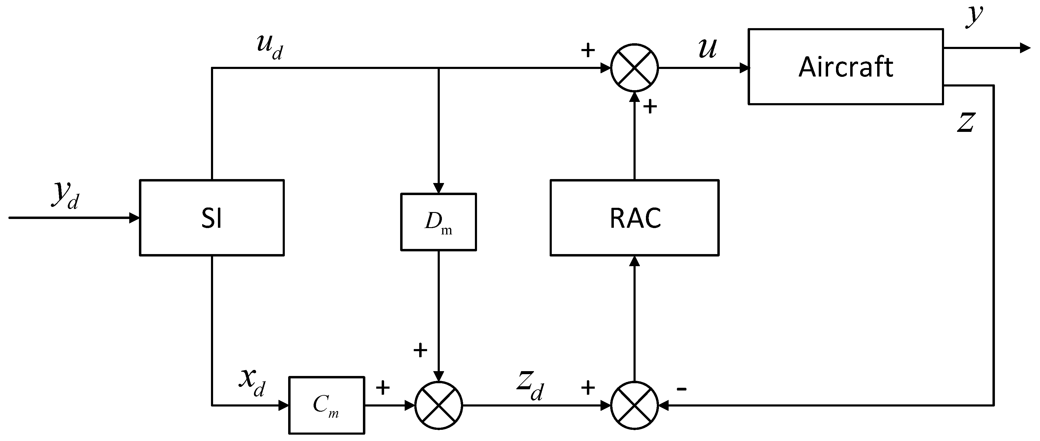
A stable inversion (SI) based robust autolanding controller (SIRAC) is proposed to improve the RAC scheme. The SI algorithm is used to enhance the trajectory tracking ability of aircraft autolanding system, which calculates the desired input and state through the desired landing trajectory. While the disturbance rejection ability is also increased due to the integration of the SI algorithm and $H_{\infty }$ synthesis.

The rest of the paper is organized, as follows: Section 2 deals with the models of the aircraft, actuator, windshear, and the desired landing trajectory used in this study. Section 3 describes the design of the SIRAC. Section 4 presents some simulations to illustrate the SIRAC performances. Section 5 summarizes the conclusions.

2. Dynamics Modelling and Problem Formulation

2.1. Aircraft Dynamics and Actuator Modelling

The dynamic model of a civil aircraft can be built via Newton law, and in normal operating conditions, such a model can be decoupled into longitudinal motion and lateral motion, as they have a slight impact on each other. For the purpose of autolanding, the longitudinal motion model is employed here [22,23], which is

$$\begin{array}{l}\dot{V}=\frac{1}{m}\left[T\cos (\alpha +{\epsilon }_T)-D-mg\sin (\gamma )\right]\\ \dot{\gamma }=\frac{1}{mV}\left[T\sin (\alpha +{\epsilon }_T)+L-mg\cos (\gamma )\right]\\ \dot{q}=\frac{M}{I_{yy}}\\ \dot{\theta }=q\end{array}$$

(1)

where $m$ is the aircraft mass, $V$ is the longitudinal speed, $\alpha$ is the angle of attack, $q$ is the pitch rate, $\theta$ is the pitch rate, $\gamma$ is the flight path angle, ${\epsilon }_T$ is the thrust inclination angle, $I_{yy}$ is the principal moment of inertia in pitch axis, $M$ is the pitching moment, and $T$, $L$, and $D$ are the thrust, lift and drag, respectively. The aerodynamics forces and moment in Equation (1) can be described, as follows:

$$\begin{array}{l}L=\frac{1}{2}\rho V^{2}S{C}_L,D=\frac{1}{2}\rho V^{2}S{C}_D\\ M=\frac{1}{2}\rho V^{2}S\overline{c}{C}_M,T=T_0+\frac{\partial T}{\partial {\delta }_t}{\delta }_t\end{array}$$

(2)

where the aerodynamic coefficients can be described, as follows:

$$\begin{array}{l}{C}_L=C_{L0}+C_L^{\alpha }\alpha +C_L^{{\delta }_e}{\delta }_e+(C_L^{\dot{\alpha }}\dot{\alpha }+C_L^{q}q)\frac{\overline{c}}{2V_0}\\ C_D=C_{D0}+C_D^{\alpha }\alpha +C_D^{{\delta }_e}{\delta }_e+(C_D^{\dot{\alpha }}\dot{\alpha }+C_D^{q}q)\frac{\overline{c}}{2V_0}\\ C_M=C_{M0}+C_M^{\alpha }\alpha +C_M^{{\delta }_e}{\delta }_e+(C_M^{\dot{\alpha }}\dot{\alpha }+C_M^{q}q)\frac{\overline{c}}{2V_0}\end{array}$$

(3)

Table 1. The Boeing 747 aircraft parameters.

Parameter	Value	Unit	Description
$m$	250,000	kg	Mass
$S$	510	m2	Wing reference area
$\overline{c}$	8.3	m	Mean aerodynamic chord
$I_{yy}$	$41.35\times {10}^6$	kg·m2	Pitch axis inertia
${\epsilon }_T$	0.044	rad	Thrust inclination angle
$C_{L0}$	1.71
$C_L^{\alpha }$	5.67	1/rad	Angle of attack derivative for lift
$C_L^{{\delta }_e}$	0.36	1/rad	Elevator variation derivative for lift
$C_L^{\dot{\alpha }}$	6.7	s/rad	Angle of attack rate derivative for lift
$C_L^q$	5.65	s/rad	Pitch rate derivative for lift
$C_{D0}$	0.263
$C_D^{\alpha }$	1.13	1/rad	Angle of attack derivative for drag
$C_D^{{\delta }_e}$	0	1/rad	Elevator variation derivative for drag
$C_D^{\dot{\alpha }}$	0	s/rad	Angle of attack rate derivative for drag
$C_D^q$	0	s/rad	Pitch rate derivative for drag
$C_{M0}$	−0.093
$C_M^{\alpha }$	−1.45	1/rad	Angle of attack derivative for moment
$C_M^{{\delta }_e}$	−1.40	1/rad	Elevator variation derivative for moment
$C_M^{\dot{\alpha }}$	−3.3	s/rad	Angle of attack rate derivative for moment
$C_M^q$	−21.4	s/rad	Pitch rate derivative for moment
$T_0$	382.572	kN
$\frac{\partial T}{\partial {\delta }_t}$	7801.63	kN/rad	Throttle variation derivative for thrust

provides the corresponding parameters of the civil aircraft Boeing 747 [24], which are used for simulations and analysis. Equation (1) can be trimmed and linearized according to small perturbation linearization theory.

Table 2. The trim conditions.

Parameters	Value	Unit	Description
$h$	0	m	Altitude
$V_0$	67.4	m/s	Initial speed
$\rho$	1.225	kg/m3	Air density
${\alpha }_0$	0.148	rad	Trim angle of attack
${\gamma }_0$	0	rad	Trim flight path angle

lists the trim conditions.

The elevator actuator and engine models are listed, as follows:

$$\frac{{\delta }_e}{{\delta }_{ec}}=\frac{10}{s+10}$$

(4)

$$\frac{{\delta }_t}{{\delta }_{tc}}=\frac{0.25}{s+0.25}$$

(5)

where ${\delta }_e$ is the elevator deflection angle, ${\delta }_t$ is the throttle position changing, and ${\delta }_{ec}$ and ${\delta }_{tc}$ are commands. The maximum deflections and rates of elevator and engine are limited in order to ensure the aircraft’s safety and comfortability, which are listed in

Table 3. The maximum deflections and rates.

${\mathit{\delta }}_{\mathit{e}}$	$\dot{{\mathit{\delta }}_{\mathit{e}}}$	${\mathit{\delta }}_{\mathit{t}}$	$\dot{{\mathit{\delta }}_{\mathit{t}}}$
0.35(rad)	0.26(rad/s)	0.088(rad)	0.017(rad/s)

[25].

Combining the linearized aircraft model and the actuators model, the linearized state equation can be written, as follows:

$$\dot{x}(t)=Ax(t)+Bu(t)$$

(6)

where $x(t)={[{\delta }_e(t),{\delta }_t(t),V(t),\gamma (t),q(t),\theta (t),h(t)]}^T$, $u(t)={[{\delta }_{ec}(t),{\delta }_{tc}(t)]}^T$, and

$$A=\left[\begin{array}{ccccccc}-10& 0& 0& 0& 0& 0& 0\\ 0& -0.25& 0& 0& 0& 0& 0\\ 0& 0.98& -0.04& -10.56& 0& -21.64& 0\\ 0& 0& 0& -0.49& 0.03& 0.49& 0\\ 0& 0.01& 0& 0.42& -0.38& -0.42& 0\\ 0& 0& 0& 0& 1& 0& 0\\ 0& 0& 0& 221& 0& 0& 0\end{array}\right],B=\left[\begin{array}{cc}10& 0\\ 0& 0.25\\ 0& 0\\ 0& 0\\ 0& 0\\ 0& 0\\ 0& 0\end{array}\right]$$

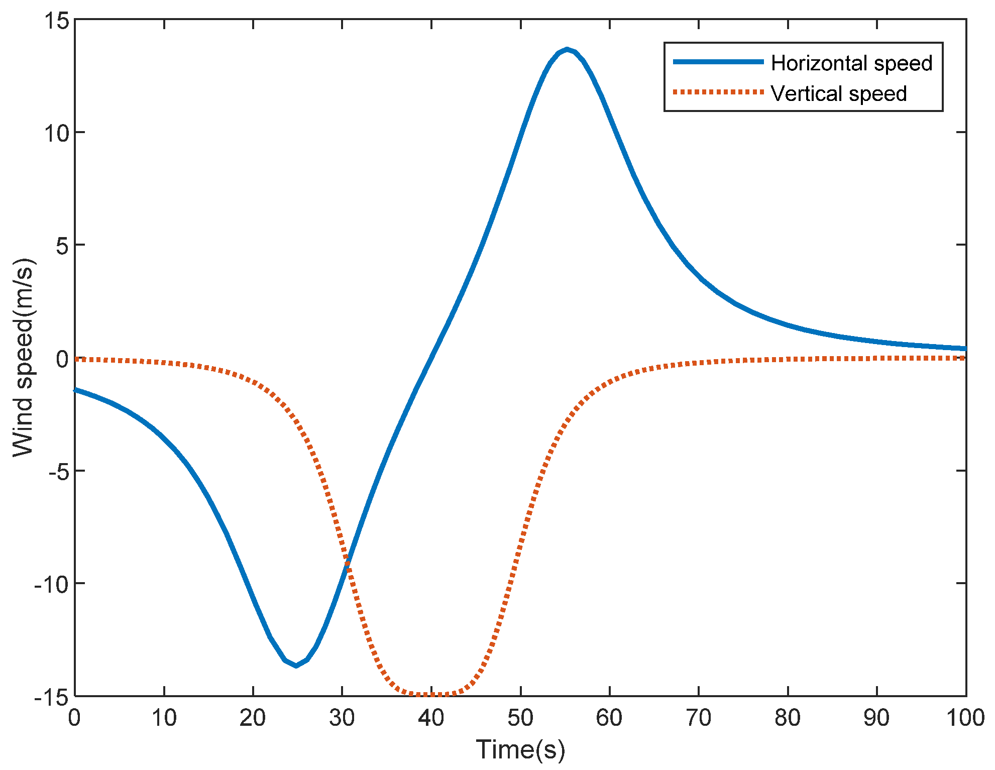
2.2. Windshear Model

Windshear is a rapid variation in the velocity and direction of air flows. If the diameter of the windshear is less than 4 km, then it is called a microburst, otherwise a macroburst. Although windshear might last only a few minutes, it is one of the most dangerous factors in the takeoff and landing of an aircraft at low altitude because of its extreme speed and variation.

Researchers have developed many different models of windshear. Woodfield and Wood developed the vortex-ring model [26]. This paper uses the simplified vortex-ring downburst model [27] in simulations. As the lateral motion is ignored, the horizontal and vertical wind speeds are given, as follows:

$$\begin{array}{c}{W}_x=f_x\left(\frac{100}{{[(x-3D/2)/200]}^2+10}-\frac{100}{{[(x-D/2)/200]}^2+10}\right)\\ W_h=-f_h\left(\frac{0.4h}{{\left[(x-D)/400\right]}^2+10}\right)\end{array}$$

(7)

where $W_x$ is the horizontal wind speed, $W_h$ is the vertical wind speed, $D=V_{0}T/2$, $x=V_{0}t$, $V_0$ is the approaching speed, $T$ is the total time during which the aircraft flies in the windshear, and $f_x$ and $f_h$ are the strengths of the windshear.

As the windshear speeds will influence the aircraft landing maneuver, Equation (7) needs to be embedded into the aircraft dynamics in the flight simulation. Additionally, the longitudinal motion equations can be written, as follows:

$$\begin{array}{c}\dot{x}=V\cos (\gamma )+W_x\\ \dot{h}=V\sin (\gamma )+W_h\\ \dot{V}=\frac{1}{m}\left[T\cos (\alpha +{\epsilon }_T)-D-mg\sin (\gamma )-m\dot{W_x}\cos (\gamma )-m\dot{W_h}\sin (\gamma )\right]\\ \dot{\gamma }=\frac{1}{mV}\left[T\sin (\alpha +{\epsilon }_T)+L-mg\cos (\gamma )+m\dot{W_x}\sin (\gamma )-m\dot{W_h}\cos (\gamma )\right]\end{array}$$

(8)

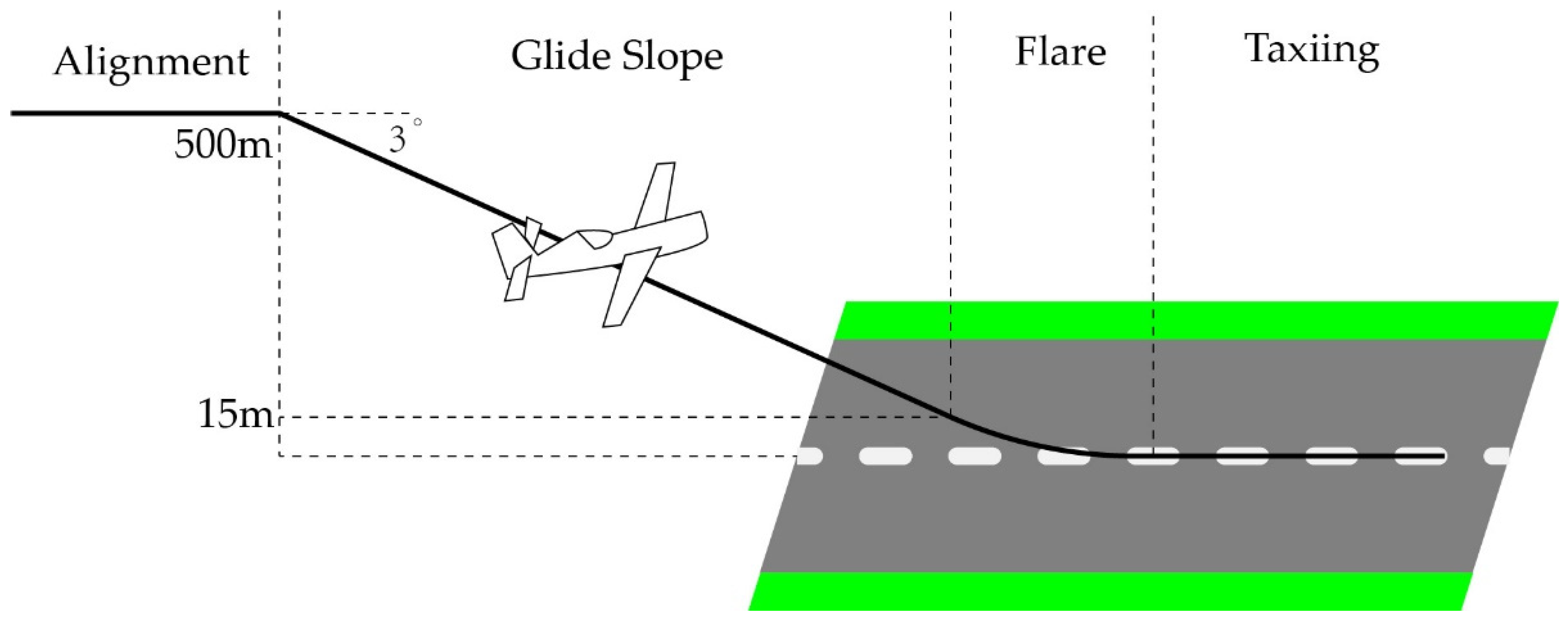
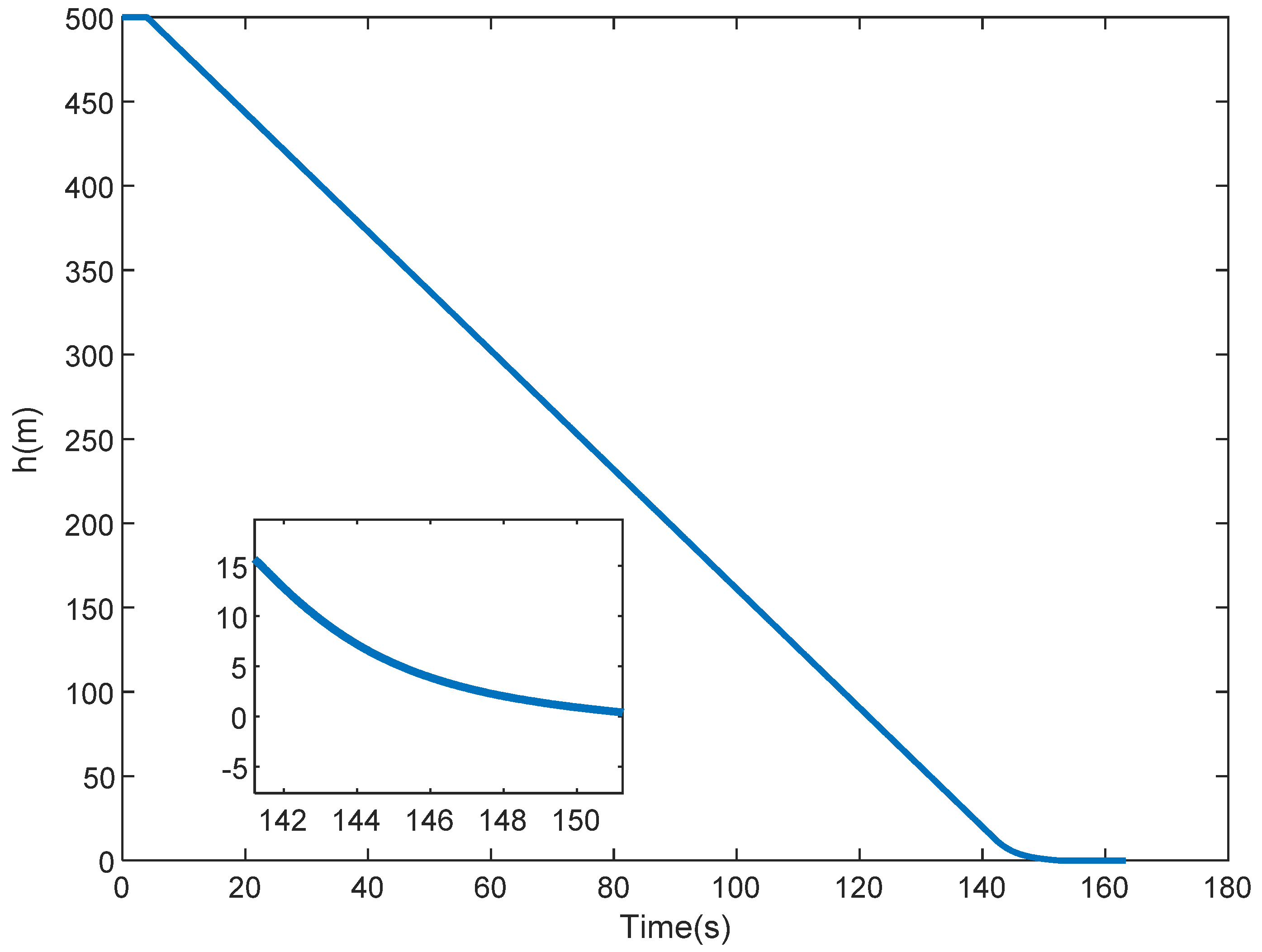
2.3. The Desired Landing Trajectory

In the alignment phase, the aircraft altitude will be around 500 m. Additionally, it keeps at a constant speed. In this case, the approaching speed is selected as 67.4 m/s. After that, the aircraft will enter the glide slope mode, when the approach path reaches the desired glide path. In this mode, the flight path angle should be kept at −3 deg and the gliding velocity should be maintained at a constant value. The aircraft enters the flare phase when the altitude is around 15 m. The aircraft will gradually approach the ground and the vertical speed will be reduced to 0.3 m/s at the touch down point.

From above analysis, two variables need to be controlled, such that the aircraft follows the desired trajectory: one variable is the longitudinal speed $V$ and another is the altitude $h$. According to the civil aircraft landing requirements, the desired longitudinal speed $V_d$ is almost constant during the landing stage. As the vertical speed is very small, the horizontal speed $V_x$ is assumed to be equal to the longitudinal speed $V_d$, that is

$$V_x\approx V_d=67.4 \mathrm{m}/\mathrm{s}$$

(9)

The desired altitude trajectory $h_d$ includes two parts: glide slope and flare segment. In the glide slope, the flight path angle is −3 deg, so the desired trajectory is

$$h_d(t)=-\tan (3^{\circ })V_{x}t=-\tan (3^{\circ })V_{d}t$$

(10)

In the flare segment, the desired trajectory is chosen as [28]

$$h_d(t)=\frac{k_1}{k_2^2}{e}^{-k_2{V}_{x}t}-\frac{k_1}{4k_2^2}{e}^{-2k_2{V}_{x}t}+k_3{V}_{x}t+k_4=\frac{k_1}{k_2^2}{e}^{-k_2{V}_{d}t}-\frac{k_1}{4k_2^2}{e}^{-2k_2{V}_{d}t}+k_3{V}_{d}t+k_4$$

(11)

where the $k_1,\cdot \cdot \cdot ,k_4$ meet the following equations:

$$\begin{array}{c}{\dot{h}}_d(0)=V_d\sin (3^{\circ }),h_d(0)=15m\\ {\dot{h}}_d(t_a)=0.3m/s,h_d(t_a)=0\end{array}$$

(12)

where $t_a$ is the total time of the flare segment, which is chosen as $t_a=10s$. We choose the initial $k_0=\left[k_{1_0},k_{2_0},k_{3_0},k_{4_0}\right]=\left[0.0001,0.01,0,5\right]$ and the allowable error is ${10}^{-4}$ in order to find $k_1,\cdot \cdot \cdot ,k_4$. Using the function $fsolve(·)$ in $Matlab$ to get the following results:

$$\begin{array}{l}{k}_1=0.0006,k_2=0.0056\\ k_3=-0.0031,k_4=1.7933\end{array}$$

Figure 2 shows the desired trajectory of the altitude $h_d$.

3. Design of SIRAC

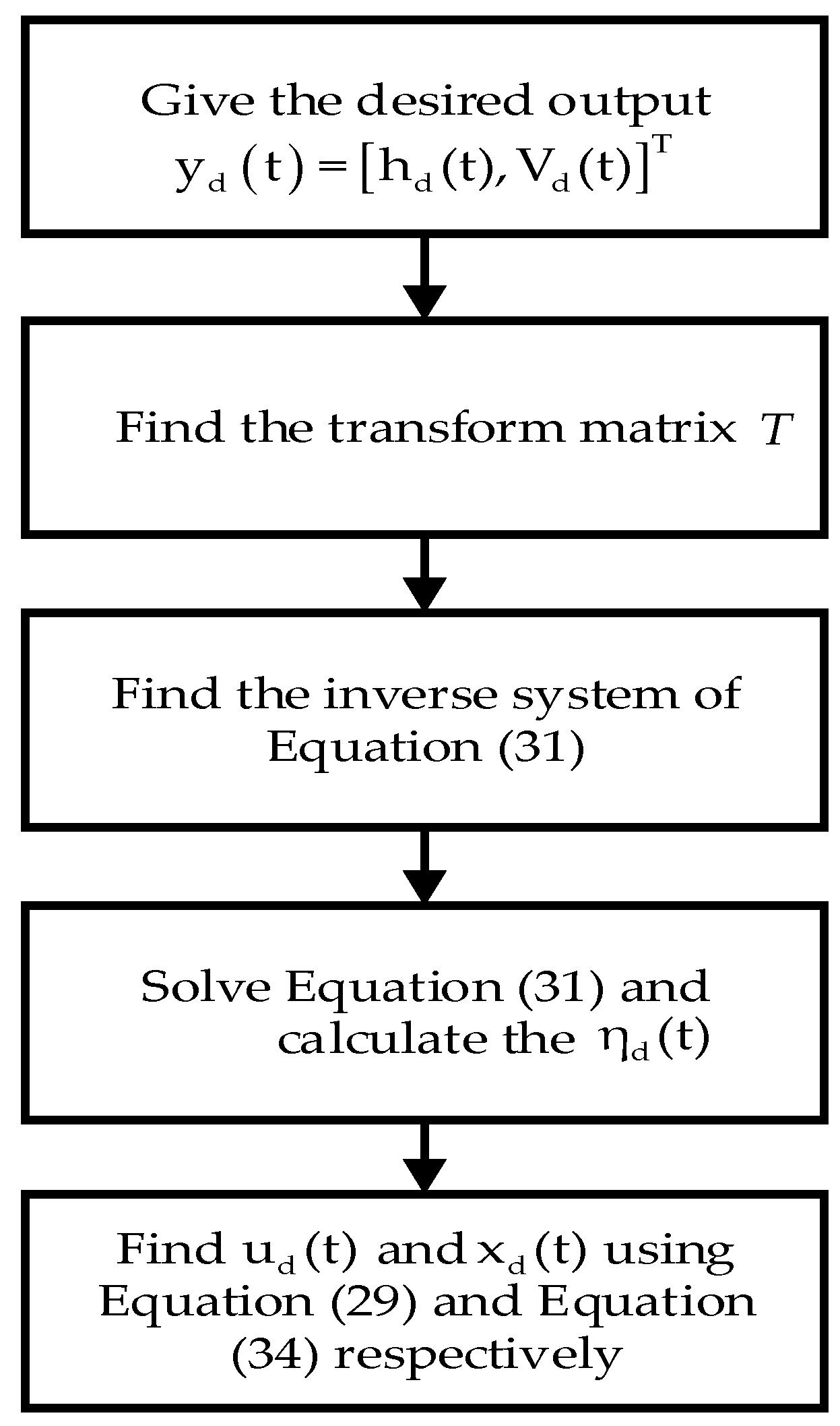
3.1. The SI Algorithm

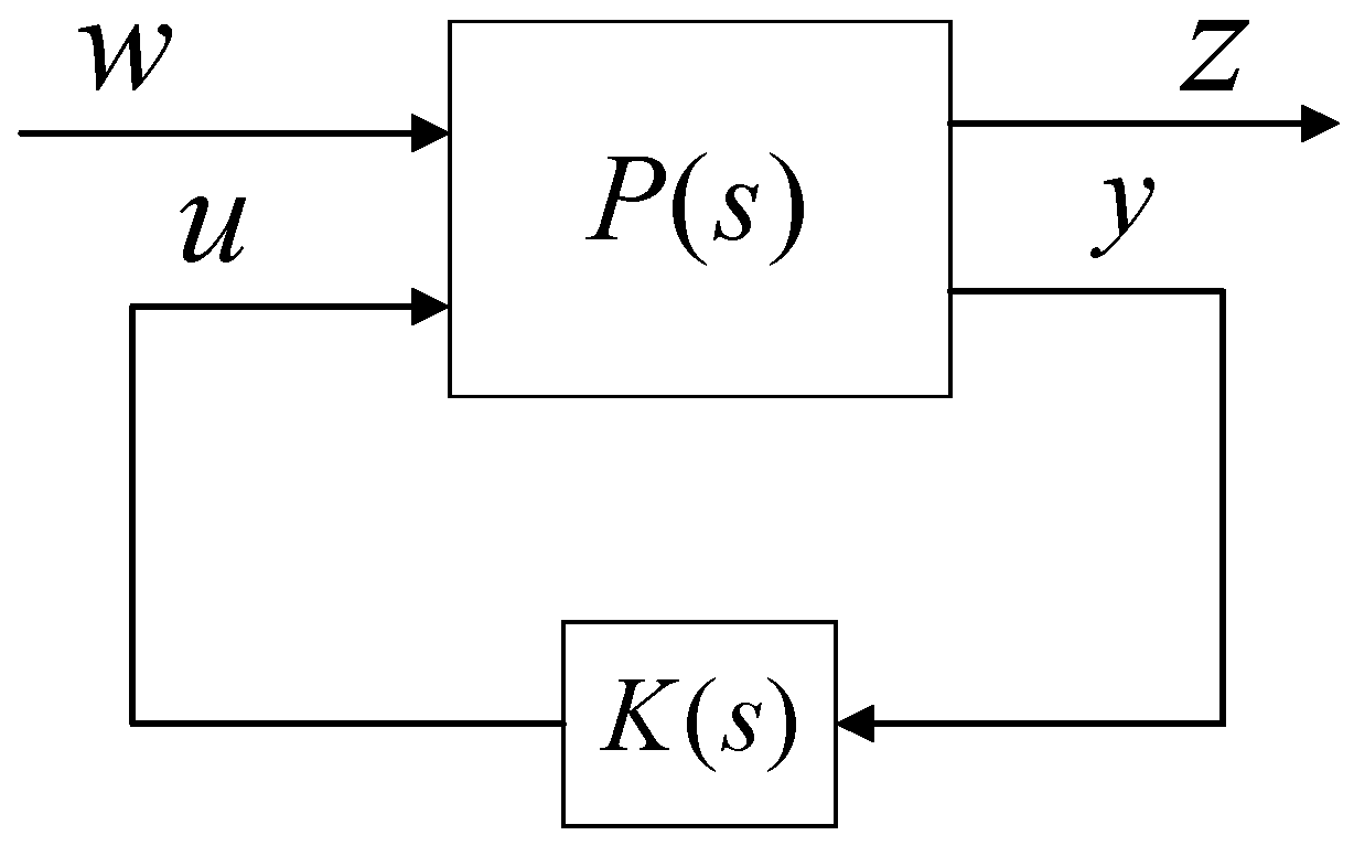
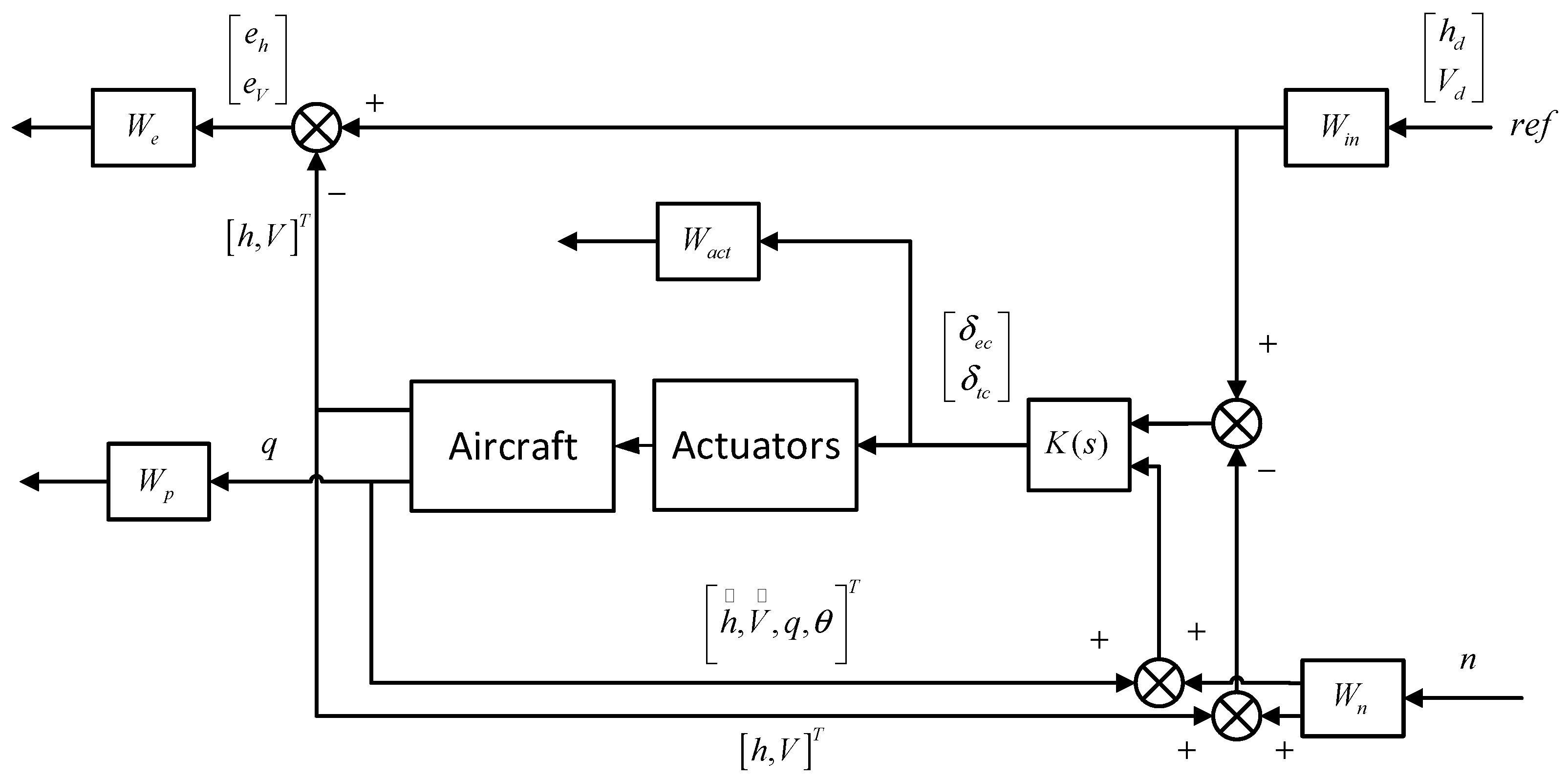
While considering the NMP linear system:

$$\begin{array}{l}\dot{x}\left(t\right)=Ax\left(t\right)+Bu\left(t\right)\\ y\left(t\right)=Cx\left(t\right)+Du\left(t\right)\\ z\left(t\right)=C_{m}x\left(t\right)+D_{m}u\left(t\right)\end{array}$$

(13)

where $x\in {ℝ}^n$, $u\in {ℝ}^p$, $y\in {ℝ}^m$, $z\left(t\right)$ is the measurement output, and $A$, $B$, $C$, $D$, $C_m$, and $D_m$ are suitable dimension matrices.

If $y_d\left(t\right)$ is the desired trajectory, the desired input $u_d(t)$ and state $x_d(t)$ meet the following equations:

$$\begin{array}{l}{\dot{x}}_d\left(t\right)=A{x}_d\left(t\right)+B{u}_d\left(t\right)\\ y_d\left(t\right)=C{x}_d\left(t\right)+D{u}_d\left(t\right)\\ z_d\left(t\right)=C_m{x}_d\left(t\right)+D_m{u}_d\left(t\right)\end{array}$$

(14)

then the $H_{\infty }$ controller can stabilize the output trajectory.

A transform of coordinates $T$ is used in order to find the inverse input-state of $\left[u_d(t),x_d(t)\right]$, such that:

$${\left[\xi \left(t\right),\eta \left(t\right)\right]}^T=Tx\left(t\right)$$

(15)

where $\xi \left(t\right)$ includes the output $y(t)$ and its time derivatives, that is,

$$\xi \left(t\right)\equiv {\left[y_1,{\dot{y}}_1,\cdots ,\frac{d^{r_1-1}{y}_1}{d{t}^{r_1-1}},y_2,{\dot{y}}_2,\cdots ,\frac{d^{r_2-1}{y}_2}{d{t}^{r_2-1}},\cdots ,y_m,{\dot{y}}_m,\cdots ,\frac{d^{r_m-1}{y}_m}{d{t}^{r_m-1}}\right]}^T$$

(16)

$$\frac{d^{r_k}{y}_k}{d{t}^{r_k}}=C_p{A}^{r_k}x(t)+C_p{A}^{r_k-1}Bu(t)$$

(17)

$$D=0$$

(18)

where $r=\left[r_1,r_2,\cdots ,r_m\right]$ is the relative degree vector and $C_p$ is the pth row of $C$. For the aircraft, the state $x(t)={\left[{\delta }_e\right(t),{\delta }_t(t),V(t),\gamma (t),q(t),\theta (t),h(t\left)\right]}^T$ and the output $y\left(t\right)={\left[h(t),V(t)\right]}^T$. According to [29], the relative degree $r=\left[3,2\right]$, so the $\xi \left(t\right)$ can be selected as:

$$\xi \left(t\right)\equiv {\left[\stackrel{}{h}\left(t\right),\dot{h}\left(t\right),\ddot{h}\left(t\right),V\left(t\right),\dot{V}\left(t\right)\right]}^T$$

(19)

Additionally, the system internal state $\eta \left(t\right)={\left[q(t),\theta (t)\right]}^T$. Now, Equation (15) can be rewritten as:

$${\left[\stackrel{}{h}\left(t\right),\dot{h}\left(t\right),\ddot{h}\left(t\right),V\left(t\right),\dot{V}\left(t\right),q\left(t\right),\theta (t)\right]}^T=Tx\left(t\right)$$

(20)

In order to find $T$, assume

$$u(t)={[{\delta }_{ec},{\delta }_{tc}]}^T={[{\delta }_e,{\delta }_t]}^T=\left[\begin{array}{ccccccc}1& 0& 0& 0& 0& 0& 0\\ 0& 1& 0& 0& 0& 0& 0\end{array}\right]x(t)$$

(21)

Substitute Equation (21) into Equation (17) yields

$$\frac{d^{r_k}{y}_k}{d{t}^{r_k}}=\left\{C_p{A}^{r_k}+C_p{A}^{r_k-1}B\left[\begin{array}{ccccccc}1& 0& 0& 0& 0& 0& 0\\ 0& 1& 0& 0& 0& 0& 0\end{array}\right]\right\}x(t)$$

(22)

According to Equations (20) and (22), we get

$$T=\left[\begin{array}{c}\begin{array}{ccccccc}0& 0& 0& 0& 0& 0& 1\end{array}\\ \left\{C_1{A}^1+C_1{A}^{0}B\left[\begin{array}{ccccccc}1& 0& 0& 0& 0& 0& 0\\ 0& 1& 0& 0& 0& 0& 0\end{array}\right]\right\}\\ \left\{C_1{A}^2+C_1{A}^{1}B\left[\begin{array}{ccccccc}1& 0& 0& 0& 0& 0& 0\\ 0& 1& 0& 0& 0& 0& 0\end{array}\right]\right\}\\ \begin{array}{ccccccc} 0& 0& 1& 0& 0& 0& 0\end{array}\\ \left\{C_2{A}^1+C_2{A}^{0}B\left[\begin{array}{ccccccc}1& 0& 0& 0& 0& 0& 0\\ 0& 1& 0& 0& 0& 0& 0\end{array}\right]\right\}\\ \begin{array}{ccccccc} 0& 0& 0& 0& 1& 0& 0\end{array}\\ \begin{array}{ccccccc} 0& 0& 0& 0& 0& 1& 0\end{array}\end{array}\right]$$

(23)

Currently, the system Equation (13) can be rewritten into the new coordinates, as:

$$\dot{\xi }\left(t\right)={\widehat{A}}_1\xi \left(t\right)+{\widehat{A}}_2\eta \left(t\right)+{\widehat{B}}_{1}u\left(t\right)$$

(24)

$$\dot{\eta }\left(t\right)={\widehat{A}}_3\xi \left(t\right)+{\widehat{A}}_4\eta \left(t\right)+{\widehat{B}}_{2}u\left(t\right)$$

(25)

where

$$\left[\begin{array}{cc}{\widehat{A}}_1& {\widehat{A}}_2\\ {\widehat{A}}_3& {\widehat{A}}_4\end{array}\right]=TA{T}^{-1},\left[\begin{array}{c}{\widehat{B}}_1\\ {\widehat{B}}_2\end{array}\right]=TB$$

(26)

Without the loss of general, assume that the desired output trajectory $y_d(t)$ and its time derivatives are specified, that is, $y^{\left(r\right)}\left(t\right)=y_d^{\left(r\right)}\left(t\right)$. Subsequently, the following steps are used to find the desired input $u_d\left(t\right)$ and desired state $x_d\left(t\right)$.

Step 1: Find the inverse system.

Equation (17) can be rewritten as:

$$y_d^{(r)}(t)={\left[{\stackrel{⃛}{h}}_d,{\ddot{V}}_d\right]}^T=A_x{x}_d\left(t\right)+B_y{u}_d\left(t\right)$$

(27)

where

$$A_x=\left[\begin{array}{c}{C}_1{A}^3\\ C_2{A}^2\end{array}\right],B_y=\left[\begin{array}{c}{C}_1{A}^{3-1}B\\ C_2{A}^{2-1}B\end{array}\right]$$

(28)

Substituting Equation (15) into Equation (27) yields

$$u_d\left(t\right)=B_y^{-1}\left[y_d^{\left(r\right)}\left(t\right)-A_{\xi }{\xi }_d\left(t\right)-A_{\eta }{\eta }_d\left(t\right)\right]$$

(29)

where $\left[A_{\xi },A_{\eta }\right]=A_x{T}^{-1}$.

Let $\xi \left(t\right)={\xi }_d\left(t\right)$ and $\eta \left(t\right)={\eta }_d\left(t\right)$, and then Equation (25) can be rewritten as:

$${\dot{\eta }}_d\left(t\right)={\widehat{A}}_3{\xi }_d\left(t\right)+{\widehat{A}}_4{\eta }_d\left(t\right)+{\widehat{B}}_2{B}_y^{-1}\left[y_d^{\left(r\right)}\left(t\right)-A_{\xi }{\xi }_d\left(t\right)-A_{\eta }{\eta }_d\left(t\right)\right]$$

(30)

Additionally, Equation (30) can be rewritten as:

$${\dot{\eta }}_d\left(t\right)={\widehat{A}}_{\eta }{\eta }_d\left(t\right)+{\widehat{B}}_{\eta }{Y}_d\left(t\right)$$

(31)

where $Y_d\left(t\right)={\left[y_d^{\left(r\right)}\left(t\right),{\xi }_d\left(t\right)\right]}^T$, ${\widehat{A}}_{\eta }={\widehat{A}}_4-{\widehat{B}}_2{B}_y^{-1}{A}_{\eta }$, and ${\widehat{B}}_{\eta }=\left[\begin{array}{cc}{\widehat{B}}_2{B}_y^{-1}& {\widehat{A}}_3-{\widehat{B}}_2{B}_y^{-1}{A}_{\xi }\end{array}\right]$. This is the inverse system.

Step 2: Calculate ${\eta }_d\left(t\right)$.

A transformation $M$ is used to decouple the system Equation (31) into a stable subsystem ${\sigma }_s\left(t\right)$ and an unstable subsystem ${\sigma }_u\left(t\right)$, that is,

$$M{\eta }_d\left(t\right)={\left[{\sigma }_s\left(t\right),{\sigma }_u\left(t\right)\right]}^T$$

(32)

If $A_s$ and $A_u$ are eigenvalues of ${\widehat{A}}_{\eta }$, then $diag(A_s,A_u)=M{\widehat{A}}_{\eta }{M}^{-1}$. Additionally, Equation (31) can be rewritten as:

$$\begin{array}{l}{\dot{\sigma }}_s\left(t\right)=A_s{\sigma }_s\left(t\right)+B_s{Y}_d\left(t\right)\\ {\dot{\sigma }}_u\left(t\right)=A_u{\sigma }_u\left(t\right)+B_u{Y}_d\left(t\right)\end{array}$$

(33)

where ${\left[B_s,B_u\right]}^T=M{\widehat{B}}_{\eta }$. The stable subsystem is integrated from $t=0$ to $t\to \infty$, while the unstable subsystem is integrated from $t=0$ to $t\to -\infty$. Subsequently, the bounded solution ${\eta }_d\left(t\right)$ can be found.

Step 3: Calculate $u_d\left(t\right)$ and $x_d\left(t\right)$.

If a bounded solution of ${\eta }_d\left(t\right)$ for the Equation (31) can be found, then the desired input $u_d\left(t\right)$ can be obtained through Equation (29), and the associated desired state $x_d\left(t\right)$ is obtained, as:

$$x_d\left(t\right)=T^{-1}\left[\begin{array}{c}{\xi }_d(t)\\ {\eta }_d(t)\end{array}\right]$$

(34)

Figure 3 shows the whole process of the SI algorithm.

3.2. Design of RAC

$H_{\infty }$ control is applied to process the wind disturbance. The system equations belonging to $P(s)$ in Figure 4 are given, as follows:

$$\begin{array}{l}\dot{x}(t)=Ax(t)+B_1(t)w(t)+B_{2}u(t)\\ z(t)=C_{1}x(t)+D_{11}w(t)+D_{12}u(t)\\ y(t)=C_{2}x(t)+D_{21}w(t)\end{array}$$

(35)

where $u(t)$ is the control signal, $w(t)$ is the exogenous input, $z(t)$ is the exogenous output, and $y(t)$ is the sensed output. Additionally, the RAC $K(s)$ can be represented, as follows:

$$\left[\begin{array}{c}{\dot{x}}_k(t)\\ u(t)\end{array}\right]=\left[\begin{array}{cc}{A}_k& B_k\\ C_k& D_k\end{array}\right]\left[\begin{array}{c}{x}_K(t)\\ y(t)\end{array}\right]$$

(36)

$$K(s)=\left[\begin{array}{cc}{A}_k& B_k\\ C_k& D_k\end{array}\right]$$

(37)

Substitute $u(t)$ in Equation (36) into Equation (35) and $y(t)$ in Equation (35) into Equation (36), the closed-loop system can be written as:

$$\left[\begin{array}{c}\dot{x}(t)\\ {\dot{x}}_k(t)\\ z(t)\end{array}\right]=\left[\begin{array}{ccc}A+B_2{D}_k{C}_2& B_2{C}_k& B_1+B_2{D}_k{D}_{21}\\ B_k{C}_2& A_k& B_k{D}_{21}\\ C_1+D_{12}{D}_k{C}_2& D_{12}{C}_k& D_{11}+D_{12}{D}_k{D}_{21}\end{array}\right]\left[\begin{array}{c}x(t)\\ x_k(t)\\ w(t)\end{array}\right]$$

(38)

Let

$$\begin{array}{l}{A}_{cl}=\left[\begin{array}{cc}A+B_2{D}_k{C}_2& B_2{C}_k\\ B_k{C}_2& A_k\end{array}\right],B_{cl}=\left[\begin{array}{c}{B}_1+B_2{D}_k{D}_{21}\\ B_k{D}_{21}\end{array}\right]\\ C_{cl}=\left[\begin{array}{cc}{C}_1+D_{12}{D}_k{C}_2& D_{12}{C}_k\end{array}\right],D_{cl}=\left[D_{11}+D_{12}{D}_k{D}_{21}\right]\end{array}$$

(39)

and

$$\underset{\_}{S}(P,K)=\left[\begin{array}{cc}{A}_{cl}& B_{cl}\\ C_{cl}& D_{cl}\end{array}\right]$$

(40)

The desired performance criterion to be minimized can be taken as a $H_{\infty }$ norm of the closed loop transfer function. Hence, the cost function takes the following form [30]

$$J_{\infty }(K)={\Vert \underset{\_}{S}(P,K)\Vert }_{\infty }$$

(41)

where $K(s)$ should make the closed-loop system stable and satisfy the following $H_{\infty }$ norm constraints

$$J_{\infty }(K)<\gamma ,\gamma >0$$

(42)

Linear Matrix Inequalities (LMIs) are used to solve the $H_{\infty }$ optimal control problem for a minimum $\gamma$ without losing convexity in order to find the controller $K(s)$. Next, we give three steps to find the controller $K(s)$ [31].

Step 1: Find symmetric matrices $R$ and $S$.

$${\left[\begin{array}{cc}{N}_R& 0\\ 0& I\end{array}\right]}^T\left[\begin{array}{ccc}AR+R{A}^T& *& *\\ C_{1}R& -\gamma I& *\\ B_1^T& D_{11}^T& -\gamma I\end{array}\right]\left[\begin{array}{cc}{N}_R& 0\\ 0& I\end{array}\right]<0$$

(43)

$${\left[\begin{array}{cc}{N}_S& 0\\ 0& I\end{array}\right]}^T\left[\begin{array}{ccc}{A}^{T}S+SA& *& *\\ B_1^{T}S& -\gamma I& *\\ C_1& D_{11}& -\gamma I\end{array}\right]\left[\begin{array}{cc}{N}_S& 0\\ 0& I\end{array}\right]<0$$

(44)

$$\left[\begin{array}{cc}R& I\\ I& S\end{array}\right]\ge 0$$

(45)

where $N_R$ is the basis of the null space of ${\left[\begin{array}{cc}{B}_2& D_{12}\end{array}\right]}^T$, and $N_S$ is the basis of the null space of $\left[\begin{array}{cc}{C}_2& D_{21}\end{array}\right]$.

Step 2: Find symmetric positive definite matrix $X$.

When the $R$ and $S$ are found, we solve $M{N}^T=I-RS$, and let

$$X{F}_1=F_2$$

(46)

where

$$F_1=\left[\begin{array}{cc}R& I\\ M^T& 0\end{array}\right],F_2=\left[\begin{array}{cc}I& S\\ 0& N^T\end{array}\right]$$

(47)

Step 3: Find the controller $K(s)$.

When the $X$ is found, according to the bounded real lemma, if $\underset{\_}{S}(P,K)$ is stable and $J_{\infty }(K)<\gamma$, then $X$ should satisfy the LMI

$$\left[\begin{array}{ccc}{A}_{cl}^{T}X+X{A}_{cl}& *& *\\ B_{cl}^{T}X& -\gamma I& *\\ C_{cl}& D_{cl}& -\gamma I\end{array}\right]<0$$

(48)

Let Inequality (48) left multiplies $diag\left(F_1^T,I,I\right)$ and right multiplies $diag\left(F_1,I,I\right)$ and substitute $A_{cl}$, $B_{cl}$, $C_{cl}$, and $D_{cl}$ into Inequality (48) yields

$$\left[\begin{array}{cccc}\left(AR+R{A}^T+B_2\widehat{C}+{(B_2\widehat{C})}^T\right)& *& *& *\\ \widehat{A}+{(A+B_2\widehat{D}{C}_2)}^T& A^{T}S+SA+\widehat{B}{C}_2+{(\widehat{B}{C}_2)}^T& *& *\\ B_1^T+{(B_2\widehat{D}{D}_{21})}^T& {(S{B}_1+\widehat{B}{D}_{21})}^T& -\gamma I& *\\ C_{1}R+D_{12}\widehat{C}& C_1+D_{12}\widehat{D}{C}_2& D_{11}+D_{12}\widehat{D}{D}_{21}& -\gamma I\end{array}\right]<0$$

(49)

where $diag(·)$ represents diagonal matrix and

$$\begin{array}{l}\widehat{A}=S(A+B_2{D}_k{C}_2)R+N{B}_k{C}_{2}R+S{B}_2{C}_k{M}^T+N{A}_k{M}^T\\ \widehat{B}=S{B}_2{D}_k+N{B}_k\\ \widehat{C}=D_k{C}_{2}R+C_k{M}^T\\ \widehat{D}=D_k\end{array}$$

(50)

Now, the controller $K(s)$ can be constructed, as follows:

$$\begin{array}{l}{D}_k=\widehat{D}\\ C_k=(\widehat{C}-D_k{C}_{2}R)(M^T{)}^{-1}\\ B_k=N^{-1}(\widehat{B}-S{B}_2{D}_k)\\ A_k=N^{-1}[\widehat{A}-S(A+B_2{D}_k{C}_2)R](M^T{)}^{-1}-B_k{C}_{2}R(M^T{)}^{-1}-N^{-1}S{B}_2{C}_k\end{array}$$

(51)

The above method has been expanded into RAC design. Figure 5 shows the interconnected structure of the general plant for the RAC.

Where $n$ is the sensors noises, $W_{in}$, $W_p$, $W_e$, $W_{act}$, and $W_n$ are the weighting functions. In this case, $h$ and $V$ are the variables to be controlled. The weighting functions are selected, as follows, according to the specifications to achieve the desired performances. There are two main tuning criteria that are used for selecting the weighting functions of the $H_{\infty }$ controller: one is the weighting functions of some components of a vector signal should be bigger if they are more important than others, the other is each component of the signal should be scaled to the same units according to the weighting functions to make these components comparable.

The altitude $h_d$ and speed $V_d$ commands are scaled by $W_{in}$ in order to normalize the reference inputs. Select the average altitude $h_{ave}=250 \mathrm{m}$ and average speed $V_{ave}=67.4 \mathrm{m}/s$, and yields:

$$W_{in}=diag(h_{ave},V_{ave})=diag(250,67.4)$$

(52)

The gain of $W_e$ should be big enough at low frequency to enable the controlled system to track ramp commands with a very small steady state error, as the altitude error $e_h$ and the speed error $e_V$ should be small, and the altitude and speed do not change quickly. Hence, the $W_e$ is selected as:

$$W_e=diag\left(20000\frac{1}{s+0.007},12000\frac{1}{s+0.002}\right)$$

(53)

where 20,000 and 12,000 are proportional gains and 1/0.007 and 1/0.002 are time constants. It is obvious that the magnitude of $W_e$ is big at low frequency, which is similar with a proportional integral (PI) element, as the integral element can eliminate the steady state error.

As the maximum pitch rate is $\pm 0.52$ rad/s [25], the weighting function of $W_p$ is selected as:

$$W_p=\frac{1}{0.052}$$

(54)

The weighting function of $W_{act}$ is applied to confine the control deflections and their rates. According to the maximum deflections and rates of elevator and engine in Table 3, the $W_{act}$ is selected as:

$$W_{act}=diag\left(\frac{1}{0.35},\frac{1}{0.26},\frac{1}{0.088},\frac{1}{0.017}\right)$$

(55)

As measurements are often corrupted with some noises, according to the measurement noise error [25], the measurement noise weighting function $W_n$ is selected, as:

$$W_n=diag\left(W_{nh},W_{n\dot{h}},W_{nV},W_{n\dot{V}},W_{nq},W_{n\theta }\right)=diag\left(0.01,0.025,0.015,0.02,\frac{0.05}{57.3},\frac{0.1}{57.3}\right)$$

(56)

Based on the above weighting functions, RAC is constructed following the preceding three steps and the matrices are given, as follows:

$$A_k=\left[\begin{array}{ccccccccc}-0.021& 0.122& 0& -0.322& 0& 0.013& 0.500& 0& 0\\ -0.209& -0.530& 2.210& 0& 0& -0.080& -0.022& 0& 0\\ 0.017& -0.164& -0.412& 0& 0& -0.473& 0.272& 0& 0\\ 0& 0& 1& 0& 0& 0& 0& 0& 0\\ 0& -1& 0& 2.210& 0& 0& 0& 0& 0\\ -758& -9167& 1957& 25512& 16767& 24.413& -144& -107& 7.402\\ -559& 315& -73& -875& -682& -4.007& -184& 4.598& 2.475\\ -0.277& -4.256& 0.779& 11.568& 12.857& -0.002& 0.003& -0.084& 0.003\\ 0.899& 0.364& -0.067& -0.991& -1.013& 0& 0& 0.006& -0.008\end{array}\right]$$

$$B_k=\left[\begin{array}{cccccc}0& 0& 0& 0& 0& 0\\ 0& 0& 0& 0& 0& 0\\ 0& 0& 0& 0& 0& 0\\ 0& 0& 0& 0& 0& 0\\ 0& 0& 0& 0& 0& 0\\ 0& 0& 0& 0& 0& 0\\ 0& 0& 0& 0& 0& 0\\ 131& -0.104& 0& 0& 0& 0\\ -0.248& 129& 0& 0& 0& 0\end{array}\right]$$

$$C_k=\left[\begin{array}{ccccccccc}-94& 1146& 244& 3189& 2096& -1.802& -18& -13& 0.925\\ -1119& 630& -146& -1750& -1365& -8.014& -368& 9.195& 4.949\end{array}\right]$$

$$D_k=\left[\begin{array}{cccccc}0& 0& 0& 0& 0& 0\\ 0& 0& 0& 0& 0& 0\end{array}\right]$$

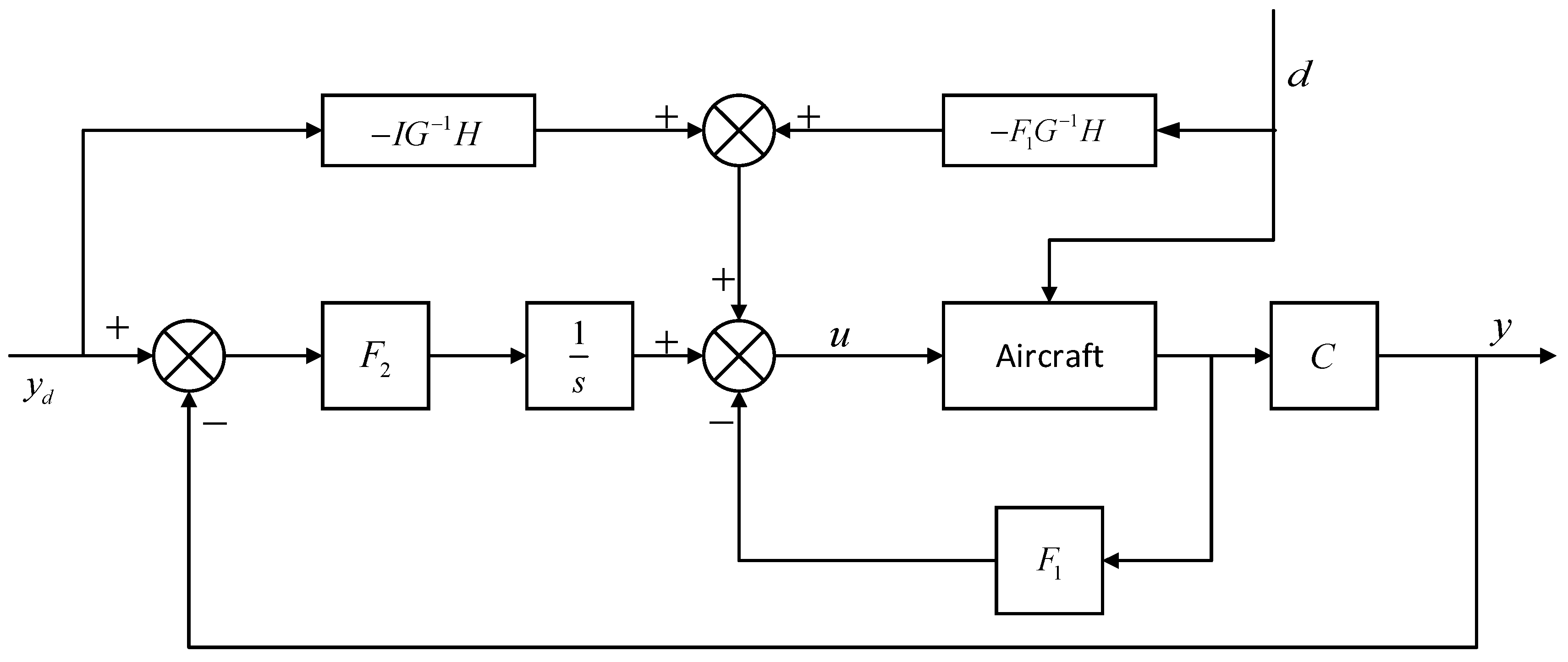
3.3. Combining the SI Algorithm and RAC

Figure 6 shows the architecture of SIRAC, which includes SI algorithm and RAC. The SIRAC can simultaneously meet trajectory tracking and disturbance rejection requirements. The desired input $u_d$ and state $x_d$ can be calculated off-line based on the desired landing trajectory while using the SI algorithm. The RAC is used to robust against the wind disturbances. The SI drives the output trajectory of the aircraft to the desired trajectory.

Now, the algorithm of the SIRAC is designed, as follows.

Step 1

Calculating $y_d={\left[h_d,V_d\right]}^T$.

Step 2

Knowing $y_d$, solve Equation (29) and Equation (34) using SI algorithm to find the $u_d$ and $x_d$.

Step 3

Knowing $u_d$ and $x_d$, solve $z_d=C_m{x}_d+D_m{u}_d$.

Step 4

Knowing $z_d$, solve $(z_d-z)$ for the input of RAC: ${[\Delta h,\Delta \dot{h},\Delta V,\Delta \dot{V},\Delta q,\Delta \theta ]}^T$.

Step 5

Knowing $(z_d-z)$, solve Equation (36) for the output of RAC: ${\left[{\delta }_{ec},{\delta }_{tc}\right]}^T$.

Step 6

Knowing ${\left[{\delta }_{ec},{\delta }_{tc}\right]}^T$, solve $u_d+{\left[{\delta }_{ec},{\delta }_{tc}\right]}^T$ for the input of the aircraft: $u$.

Step 7

Knowing $u$, solve the system equation of aircraft for $z$.

Step 8

Iterate over Step 3 to 7 until the landing process is done.

4. Simulation Analysis

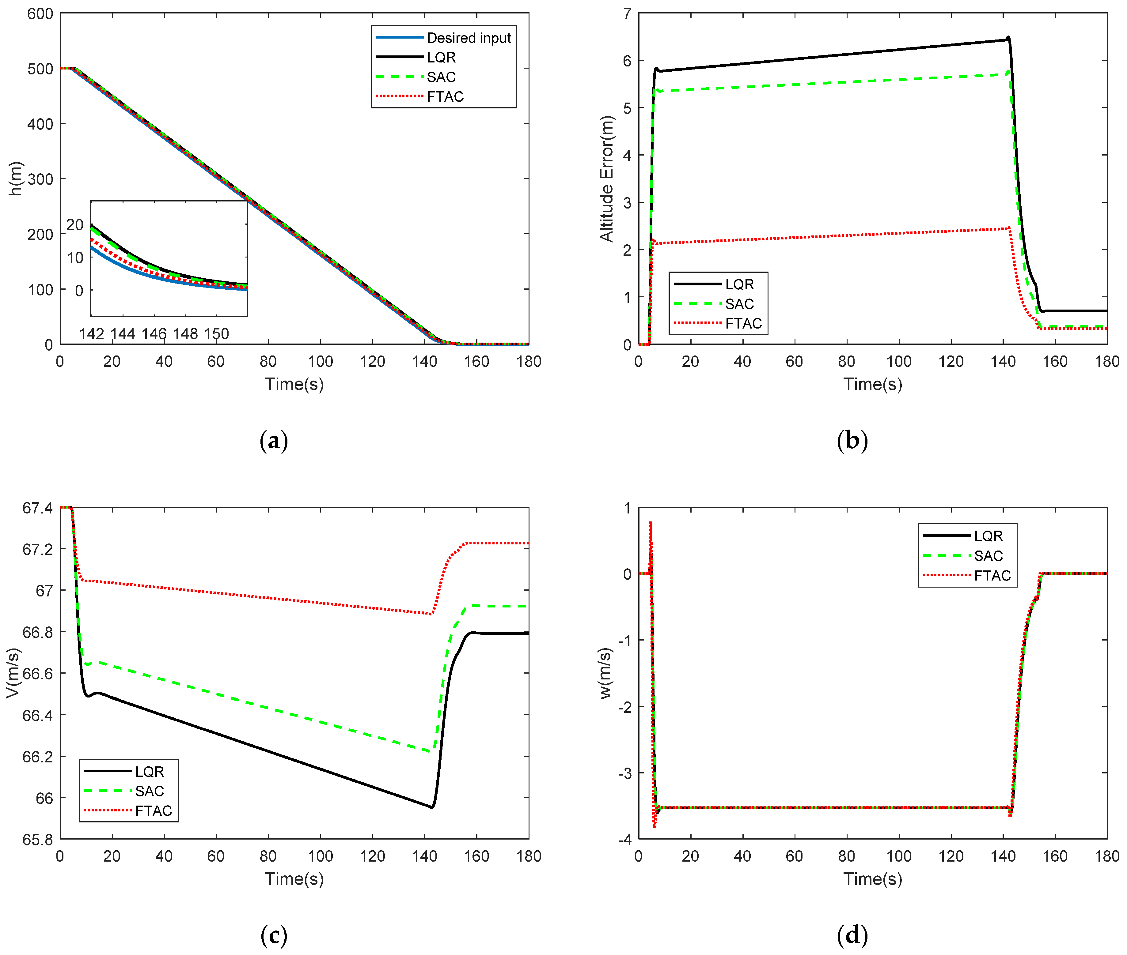
While considering the linearized aircraft model of Equation (13), matrices $A$ and $B$ have been already given in Section 2.1, and the other matrices are listed, as follows:

$$C=\left[\begin{array}{ccccccc}0& 0& 0& 0& 0& 0& 1\\ 0& 0& 1& 0& 0& 0& 0\end{array}\right],D=\left[\begin{array}{cc}0& 0\\ 0& 0\end{array}\right]$$

$$C_m=\left[\begin{array}{ccccccc}0& 0& 0& 0& 0& 0& 1\\ 0& 0& 0& 221& 0& 0& 0\\ 0& 0& 1& 0& 0& 0& 0\\ 0& 0& -0.04& -10.56& 0& -21.64& 0\\ 0& 0& 0& 0& 0& 100& 0\\ 0& 0& 0& 0& 100& 0& 0\end{array}\right],D_m=\left[\begin{array}{cc}0& 0\\ 0& 0\\ 0& 0\\ 0& 0.98\\ 0& 0\\ 0& 0\end{array}\right]$$

Additionally, $z={\left[h,\dot{h},V,\dot{V},\theta ,q\right]}^T$, $y={\left[h,V\right]}^T$. To find the $u_d$ and $x_d$ in step 2 of SIRAC algorithm, we need to know $y_d$ and its derivatives. According to Equations (10) and (11), in the glide slope,

$$\begin{array}{c}{\dot{h}}_d(t)=-\tan (3^{\circ })V_d\\ {\ddot{h}}_d(t)=0\\ {\stackrel{⃛}{h}}_d(t)=0\\ {\dot{V}}_d(t)=0\end{array}$$

(57)

In the flare segment,

$$\begin{array}{c}{\dot{h}}_d(t)=-\frac{k_1{V}_d}{k_2}{e}^{-k_2{V}_{d}t}+\frac{k_1{V}_d}{2k_2}{e}^{-2k_2{V}_{d}t}+k_3{V}_d\\ {\ddot{h}}_d(t)=k_1{V}_{{}_d}^2{e}^{-k_2{V}_{d}t}-k_1{V}_{{}_d}^2{e}^{-2k_2{V}_{d}t}\\ {\stackrel{⃛}{h}}_d(t)=-k_1{k}_2{V}_{{}_d}^3{e}^{-k_2{V}_{d}t}+2k_1{k}_2{V}_{{}_d}^3{e}^{-2k_2{V}_{d}t}\\ \dot{V_d}(t)=0\end{array}$$

(58)

where

$$\begin{array}{l}{V}_d=67.4(m/s)\\ k_1=0.0006,k_2=0.0056\\ k_3=-0.0031,k_4=1.7933\end{array}$$

The proposed method is also compared with the method in [4] for the windshear effect, which developed a linear quadratic regulator (LQR) feedforward closed-loop controller for aircraft landing. The brief introduction is as follows. More details can be found in [4].

Defining a new variable $\epsilon$ as:

$$\epsilon ={\displaystyle {\int }_0^{t_f}(y-y_d)}dt$$

(59)

where $t_f$ is the final time. While combining Equation (59) with the linearized aircraft model, it can be shown that

$$\left[\begin{array}{c}\dot{x}\\ \dot{\epsilon }\end{array}\right]=\left[\begin{array}{cc}A& 0\\ C& 0\end{array}\right]\left[\begin{array}{c}x\\ \epsilon \end{array}\right]+\left[\begin{array}{c}B\\ 0\end{array}\right]u+\left[\begin{array}{cc}E& 0\\ 0& -I\end{array}\right]\left[\begin{array}{c}d\\ y_d\end{array}\right]$$

(60)

where $d$ is the measurable disturbances. Using the assumption of constant steady-state values of $y_d$, the Equation (60) can be written, as:

$$\left[\begin{array}{c}\dot{x}\\ y-y_d\end{array}\right]=G\left[\begin{array}{c}x\\ u\end{array}\right]+H\left[\begin{array}{c}d\\ y_d\end{array}\right]$$

(61)

where

$$G=\left[\begin{array}{cc}A& B\\ C& 0\end{array}\right],H=\left[\begin{array}{cc}E& 0\\ 0& -I\end{array}\right]$$

While combining the optimal LQR with the integrator and feedforward controller, the form of the final control law is

$$u=-F_{1}x-F_2\left[{\int }_0^{t_f}(y-y_d)dt\right]-F_3\left[\begin{array}{c}d\\ y_d\end{array}\right]$$

(62)

where

$$F_3=\left[\begin{array}{cc}{F}_1& I\end{array}\right]G^{-1}H$$

It is evident that there are three terms in Equation (62). The first is the LQR, the second term is the integral control, and the third term is the feedforward of the disturbances and the desired trajectory. Figure 7 shows the block diagram of the LQR feedforward closed-loop controller.

From the view of the deflection limits of the actuators and the time response, in the glide slope, the diagonal weighting matrices $Q$ and $R$ are chosen as:

$$Q=diag\left(10,10,1,10,1,10,{10}^3,1,1\right),R=diag\left(1,{10}^7\right)$$

By solving the Riccati equation, $F_1$, $F_2$, and $F_3$ are obtained, as:

$$F_1=\left[\begin{array}{ccccccc}-8.05& 2.43& 0.77& 12.36& -123.32& 0.56& 2.38\\ -4.35& 0.00& 0.23& -1.45& -0.36& 6.53& 1.04\end{array}\right]$$

$$F_2=\left[\begin{array}{cc}0.99& 0.48\\ 0.00& 0.02\end{array}\right]$$

$$F_3=\left[\begin{array}{cccc}0.72& -2.36& 6.35& -0.23\\ 0.00& -0.02& 0.04& 0.00\end{array}\right]$$

In the flare segment, $Q$ and $R$ are chosen as:

$$Q=diag\left(1,1,1,1,1,1,10,1,1\right),R=diag\left(1,{10}^{10}\right)$$

Additionally, $F_1$, $F_2$, and $F_3$ are calculated, as:

$$F_1=\left[\begin{array}{ccccccc}-4.24& 21.43& 0.89& 2.36& -453.32& 1.03& 4.67\\ 0.00& 0.00& 0.15& 0.00& -0.66& 1.13& 0.02\end{array}\right]$$

$$F_2=\left[\begin{array}{cc}0.53& 0.86\\ 0.00& 0.00\end{array}\right]$$

$$F_3=\left[\begin{array}{cccc}0.32& -1.26& -0.89& 12.45\\ 0.00& -0.01& 0.00& 0.00\end{array}\right]$$

Now, all of the models and methods that are employed in this paper have been established. Two different scenarios are simulated while using these models and methods to demonstrate the trajectory tracking and disturbance rejection capacity of SIRAC. In the first scenario, the landing procedure of the aircraft is simulated under no wind disturbance. The results are compared with the LQR and RAC to demonstrate the trajectory tracking capacity of SIRAC. In the second scenario, the windshear effect is taken into consideration in the landing process to demonstrate the disturbance rejection capacity of SIRAC.

4.1. Scenario 1

In this scenario, the landing procedure is simulated under no wind disturbance. Figure 8a compares the actual trajectory and desired trajectory. Additionally, Figure 8b shows the errors between actual trajectory and desired trajectory. It is clearly seen that, when compared with the LQR and RAC, the actual trajectory more closely follows the desired trajectory in glide slope and flare segment while using SIRAC. Additionally, the trajectory error of SIRAC is less about 3.5 m and 3 m than the LQR and RAC, respectively. The velocity of the SIRAC is also more close to the desired velocity, which is 67.4 m/s, see Figure 8c. Based on this result, it is also expected that the descent rate is slow. As seen from Figure 8d, the descent rates of three controllers are both approximately −3.5 m/s in the glide slope and reduce to zero in the flare segment. However, at the transition, the descent rate of SIARC has a larger variation, which will enable the aircraft to track the trajectory more quickly and closely. Figure 8e shows the response of pitch angle and Figure 8f shows the response of pitch rate. It can be seen that the pitch angle and pitch rate of three controllers are smoother in the glide slope. Similarly, the variation of SIRAC is larger in the transition, as it more closely tracks the trajectory.

4.2. Scenario 2

In this scenario, the landing procedure is simulated in windshear to examine the robustness of the SIRAC. Windshear is modeled, as in Section 2.2, and the approaching speed $V_0$ is 67.4 m/s, the time $T=60 \mathrm{s}$ during which the aircraft will fly in the windshear and the strengths of the windshear $f_u$ and $f_w$ are both set as 1.5. Figure 9 shows the horizontal speed and vertical speed of the windshear, respectively. The aircraft will meet an increasing horizontal headwind and the maximum speed is about −14 m/s. Subsequently, the horizontal headwind will become horizontal downwind and the maximum speed is about 14 m/s. In the meantime, there is a downward flow, and the maximum speed is about −15 m/s.

Figure 10a shows a comparison of the altitude response between the actual trajectory and desired trajectory in a windshear environment. Additionally, Figure 10b shows the altitude error of LQR, RAC, and SIRAC. It can be seen that the largest altitude error of SIRAC is less about 10 m and 15 m than RAC and LQR in the glide slope and both 3 m in the flare segment. The velocity response of SIRAC is also smoother and more closed to desired velocity than LQR and RAC, as shown in Figure 10c. The largest velocity amplitude of SIRAC is less about 5 m/s and 6 m/s than RAC and LQR, respectively. In the windshear, it is also expected that the descent rate is slow and smooth. The descent rate of SIRAC is more closed to −3.5 m/s, as the largest error of SIRAC is about 1 m/s, RAC is 2.5 m/s, and LQR is 3 m/s, as seen from Figure 10d. The pitch angle and pitch rate responses are also shown in Figure 10e,f, respectively. It is clearly seen that when the aircraft encounters a windshear, the pitch angle response has a biggest variation 8deg while using SIRAC, 15 deg using RAC, and 18 deg using LQR. Additionally, the pitch rate also has a larger variation in the transition from initial approach to glide slope and glide slope to flare segment while using SIRAC, which means that the transition time of SIRAC is shorter. As a result, it is evident that the SIRAC provides a more precise and steady landing.

5. Conclusions

This paper presented a new approach to the ALS of the civil aircraft. Differently from the existing control methods for the autolanding system, this approach exploited the integration of the SI algorithm and $H_{\infty }$ synthesis, which could precisely track the autolanding trajectory, even in large wind disturbance. The windshear disturbance was predefined. Subsequently, the desired input and state were calculated while using SI algorithm according to the desired altitude trajectory and the desired velocity. The general plant for RAC was created. Weighting functions were selected according to the desired performances. RAC was constructed by solving the LMIs. Finally, two scenarios were simulated and studied. The simulation results demonstrated the trajectory tracking and disturbance rejection capacity of the SIRAC.

In this paper, it is assumed that the system parameters are accurate and do not change over time. However, a real system generally has system parameter uncertainties. Thus, future work will be concentrated on the robustness of the system by considering system uncertainties and turbulence. Although the paper is based on mathematical models and just shows the simulation results computed by computer, the production of prototypes has been basically completed, which indicates that our laboratories and cooperative industrial companies have reached the Technology Readiness Levels 5 (TRL5) [32].

References

1. Siegel, D.; Hansman, R.J. Development of an Autoland System for General Aviation Aircraft. Master’s Thesis, Massachusetts Institute of Technology, Cambridge, MA, USA, 2011. [Google Scholar]
2. Serra, P.; Cunha, R.; Hamel, T.; Silvestre, C.; Le Bras, F. Nonlinear image-based visual servo controller for the flare maneuver of fixed-wing aircraft using optical flow. IEEE Trans. Control Syst. Technol. 2015, 23, 570–583. [Google Scholar] [CrossRef]
3. Tapia, N.D.; Simplicio, P.; Iannelli, A.; Marcos, A. Robust flare control design using structured H∞ synthesis: A civilian aircraft landing challenge. In Proceedings of the 20th IFAC World Congress, Toulouse, France, 9–14 July 2017; pp. 3971–3976. [Google Scholar]
4. Sadat-Hoseini, H.; Fazelzadeh, S.A.; Rasti, A.; Marzocca, P. Final approach and flare control of a flexible aircraft in crosswind landings. J. Guid. Control Dyn. 2013, 36, 946–957. [Google Scholar] [CrossRef]
5. Magni, J.F. Multimodel eigenstructure assignment in flight-control design. Aerosp. Sci. Technol. 1999, 3, 141–151. [Google Scholar] [CrossRef]
6. Wang, Y.W.; Li, Q.F.; Lu, B. Automatic landing system design via multivariable model reference adaptive control. Aerosp. Syst. 2018, 1, 63–71. [Google Scholar] [CrossRef] [Green Version]
7. Rao, D.V.; Go, T.H. Automatic landing system design using sliding mode control. Aerosp. Sci. Technol. 2014, 32, 180–187. [Google Scholar]
8. Juang, J.G.; Yu, S.T. Disturbance encountered landing system design based on sliding mode control with evolutionary computation and cerebellar model articulation controller. Appl. Math. Model. 2015, 39, 5862–5881. [Google Scholar] [CrossRef]
9. Lan, C.E.; Chang, R.C. Unsteady aerodynamic effects in landing operation of transport aircraft and controllability with fuzzy-logic dynamic inversion. Aerosp. Sci. Technol. 2018, 78, 354–363. [Google Scholar] [CrossRef]
10. Juang, J.G.; Chio, J.Z. Fuzzy modelling control for aircraft automatic landing system. Int. J. Syst. Sci. 2007, 36, 77–87. [Google Scholar] [CrossRef]
11. Tamkaya, K.; Ucun, L.; Ustoglu, I. H∞-based model following method in autolanding systems. Aerosp. Sci. Technol. 2019, 94, 105379. [Google Scholar] [CrossRef]
12. Theis, J.; Ossmann, D.; Thielecke, F.; Pfifer, H. Robust autopilot design for landing a large civil aircraft in crosswind. Control Eng. Pract. 2018, 76, 54–64. [Google Scholar] [CrossRef] [Green Version]
13. Biannic, J.M.; Roos, C. Flare control law design via multi-channel ∞ synthesis: Illustration on a freely available nonlinear aircraft benchmark. In Proceedings of the 2015 American Control Conference (ACC), Chicago, IL, USA, 1–3 July 2015; pp. 1303–1308. [Google Scholar]
14. Shevchenko1, A.; Pavlov, B.; Nachinkina, G. Methods for predicting unsteady takeoff and landing trajectories of the aircraft. In Proceedings of the AIPC, Sydney, Australia, 2–5 July 2017; Volume 1798. [Google Scholar]
15. Clean Sky. Available online: https://www.cleansky.eu/ (accessed on 2 February 2020).
16. Devasia, S.; Chen, D.; Paden, B. Nonlinear inversion-based output tracking. IEEE Trans. Autom. Control 1996, 41, 930–942. [Google Scholar] [CrossRef]
17. Chen, D.; Paden, B. Stable inversion of nonlinear non-minimum phase systems. Int. J. Control 1996, 64, 81–97. [Google Scholar] [CrossRef]
18. Olivier, B.; Guaraci, J.; Robert, S. A stable inversion method for feedforward control of constrained flexible multibody systems. ASME J. Comput. Nonlinear Dyn. 2013, 9, 1–7. [Google Scholar]
19. Maghzaoui, C.; Jerbi, H.; Abdelkrim, M. A MIMO time-varying system control via a stable dynamic inversion methodology: Case of an induction machine. In Proceedings of the Computational Intelligence, Communication Systems and Networks, International Conference, Bali, Indonesia, 26–28 July 2011; pp. 146–151. [Google Scholar]
20. Zhang, J.; Zhang, P. Precise decoupling tracking of airspeed and altitude for UAV based on causal solution of stable inversion. Chin. J. Aeronaut. 2009, 22, 307–315. [Google Scholar]
21. Mancisidor, J.; Pena-Sevillano, A.; Barcena, R.; Franco, O.; Munoa, J.; De Lacalle, L.N.L. Comparison of model free control strategies for chatter suppression by an inertial actuator. Int. J. Mechatron. Manuf. Syst. 2019, 12, 164–179. [Google Scholar]
22. Bryson, A.E. Control of Spacecraft and Aircraft; Princeton University Press: Princeton, NJ, USA, 1994; pp. 137–155. [Google Scholar]
23. Roskam, J. Airplane Flight Dynamics and Automatic Flight Controls: Part I; Design, Analysis and Research Corporation: Lawrence, KS, USA, 2001; Volume 1, pp. 65–182. [Google Scholar]
24. McLean, D. Automatic Flight Control System; Prentice Hall: Hertfordshire, NJ, USA, 1990; pp. 537–576. [Google Scholar]
25. Parkinson, B.W.; O’Connor, M.L.; Fitzgibbon, K.T. Aircraft Automatic Approach and Landing Using GPS. In Global Positioning System: Theory and Applications; American Institute of Aeronautics and Astronautics, Inc.: Reston, VA, USA, 1996; Volume 2, pp. 397–425. [Google Scholar]
26. Woodfield, A.; Woods, J. Worldwide Experience of Wind Shear during 1981–1982. Technical Report; Royal Aircraft Establishment Bedford: Bedford, UK, 1983. [Google Scholar]
27. Zhao, Y. Optimal Control of an Aircraft Flying through a Downburst. Ph.D. Thesis, Stanford University, Stanford, CA, USA, 1989. [Google Scholar]
28. Thomas, R.; Stephen, C. Review of the Carrier Approach Criteria for Carrier-Based Aircraft Phase I. Naval Air Syst. Command. 2002, 71, 12–24. [Google Scholar]
29. Wang, J.-G.; Dong, X.-M.; Xue, J.-P. Aircraft longitudinal automatic landing control law design based on stable inversion. Flight Dyn. 2011, 29, 33–36. [Google Scholar]
30. Zhou, K.; Doyle, J.C.; Glover, K. Robust and Optimal Control; Prentice Hall: Bergen, NJ, USA, 1996. [Google Scholar]
31. Scherer, C.; Gahinet, P.; Chilali, M. Multiobjective output-feedback control via LMI optimization. IEEE Trans. Autom. Control 1997, 42, 896–911. [Google Scholar] [CrossRef]
32. Pinilla, L.S.; Rodríguez, R.L.; Gandarias, N.T.; De Lacalle, L.N.L.; Farokhad, M.R. TRLs 5–7 Advanced Manufacturing Centres, Practical Model to Boost Technology Transfer in Manufacturing. Sustainability 2019, 11, 4890. [Google Scholar] [CrossRef] [Green Version]
Figure 1. Illustration of landing maneuver.
Applsci 10 01224 g001
Figure 2. The desired trajectory of the altitude.
Applsci 10 01224 g002
Figure 3. Flowchart of the SI algorithm.
Applsci 10 01224 g003
Figure 4. Generalized P-K form.
Applsci 10 01224 g004
Figure 5. Interconnected structure of the general plant.
Applsci 10 01224 g005
Figure 6. The stable inversion (SI) based robust autolanding controller (SIRAC) architecture.
Applsci 10 01224 g006
Figure 7. Block diagram of the linear quadratic regulator (LQR) feedforward closed-loop controller.
Applsci 10 01224 g007
Figure 8. Scenario 1–No wind disturbance, (a) Altitude response (b) Altitude error. (c) Velocity response (d) Descent rate response. (e) Pitch angle response. (f) Pitch rate response.
Applsci 10 01224 g008aApplsci 10 01224 g008b
Figure 9. Windshear.
Applsci 10 01224 g009
Figure 10. Scenario 2–Landing in Windshear. (a) Altitude response (b) Altitude error. (c) Velocity response (d) Descent rate response. (e) Pitch angle response. (f) Pitch rate response.
Applsci 10 01224 g010