Article

Third-Octave and Bark Graphic-Equalizer Design with Symmetric Band Filters

Acoustics Laboratory, Department of Signal Processing and Acoustics, Aalto University, FI-02150 Espoo, Finland
*
Author to whom correspondence should be addressed.
Appl. Sci. 2020, 10(4), 1222; https://doi.org/10.3390/app10041222
Submission received: 3 December 2019 / Revised: 10 January 2020 / Accepted: 5 February 2020 / Published: 11 February 2020
(This article belongs to the Special Issue Digital Audio Effects)

Abstract

:
This work proposes graphic equalizer designs with third-octave and Bark frequency divisions using symmetric band filters with a prescribed Nyquist gain to reduce approximation errors. Both designs utilize an iterative weighted least-squares method to optimize the filter gains, accounting for the interaction between the different band filters, to ensure excellent accuracy. A third-octave graphic equalizer with a maximum magnitude-response error of 0.81 dB is obtained, which outperforms the previous state-of-the-art design. The corresponding error for the Bark equalizer, which is the first of its kind, is 1.26 dB. This paper also applies a recently proposed neural gain control in which the filter gains are predicted with a multilayer perceptron having two hidden layers. After the training, the resulting network quickly and accurately calculates the filter gains for third-order and Bark graphic equalizers with maximum errors of 0.86 dB and 1.32 dB, respectively, which are not much more than those of the corresponding weighted least-squares designs. Computing the filter gains is about 100 times faster with the neural network than with the original optimization method. The proposed designs are easy to apply and may thus lead to widespread use of accurate auditory graphic equalizers.

1. Introduction

The design of digital graphic equalizers (GEQ) has advanced considerably during the past five years [1,2,3]. Much research has been conducted to improve both the cascade [1,4,5,6,7] and the parallel GEQs [8,9,10,11,12,13]. Currently, for both octave and third-octave bands, designing either a cascade [3,6] or a parallel GEQ [10,11,13] having a maximum error of 1 dB, often considered sufficient for Hi-Fi audio, is possible. This work considers the design of a cascade GEQ having an auditory frequency resolution that is similar to human hearing, such as the third-octave and the Bark frequency divisions.
Quite often, auditory filters such as Bark filters are implemented using a filter bank that decomposes the input signal into different frequency bands by using bandpass filters [14,15,16]. Bark band GEQs, on the other hand, are rare. We previously implemented a very high-order Bark GEQ in [17], where the goal was to simulate how background noise masks music being listened to with different types of headphones. The masking-threshold analysis [18] was carried out using Bark bands, after which the music was suppressed based on the masking properties of the noise. This led to the need for a high-order GEQ able to essentially suppress individual Bark bands by at least 50 dB. The implementation, however, was rather unpractical, since the order of the GEQ can be several hundreds.
This paper extends the work on neurally-controlled graphic equalizers introduced in [19] and continued in the 22nd International Conference on Digital Audio Effects [20]. The first of these publications was essentially a proof of concept for controlling the filter gains of a ten-band octave GEQ using a neural network, which handled the optimization calculation [19]. The second paper extended the neurally-controlled equalizer (EQ) method to the widely used third-octave GEQ design [20], where the 31 EQ bands also loosely approximated the bandwidths of human auditory filters [21].
Compared to our previous conference paper [20], this article presents an improved design method using second-order band filters with a symmetric shape on the logarithmic frequency scale, which was recently proposed for an octave GEQ [22]. The proposed design allows the parametric EQ used as band filters in the GEQ to have a controllable gain at the Nyquist limit, in contrast to the earlier designs that forced the Nyquist gain to one (i.e., 0 dB) [3]. Furthermore, this paper extends both the weighted least-squares (WLS) GEQ design method and the neurally-controlled EQ method to operate in Bark bands, which are a more accurate approximation of the human auditory resolution than the third-octave bands [23].
Currently, two important metrics in GEQ design are accuracy and computational complexity. Both aspects have an impact when a GEQ is controlled by a computer in automated tasks without a human listener fine-tuning the gains, e.g., when equalizing music to be above a masking threshold in time varying noise [24,25]. Previous GEQs that are not very accurate (see the measurements, e.g., in [10]) have typically required a human operator to listen to the effect of the command gains as he/she controls them, since the accuracy of different command gain settings, as well as the visual feedback of the command gain sliders can be highly inaccurate. One of the goals of this work was to get the proposed neurally controlled GEQs to provide the accuracy and speed necessary to be used in automated tasks requiring fast updating of the gains, even hundreds of times per second.
The rest of this paper is organized as follows. Section 2 briefly recapitulates the design of a cascade third-octave GEQ that is approximated with the neural network. Section 3 describes the symmetric parametric EQ filters and the improved GEQ design called the symmetric graphic equalizer (SGE), which is based on an iterative WLS method, and shows how the method is applied to design third-octave and Bark band equalizers. Section 4 discusses the structure and training of a neural network used to update the filter gains rapidly. Section 5 shows the design and computational results and compares them with previous work. Section 6 concludes the paper.

2. Accurate Graphic Equalizer Design and Neural Control

Second-order infinite impulse response (IIR) filters, one per controllable band, are connected in series to form a cascade GEQ, as illustrated in Figure 1. The overall transfer function of the cascade GEQ is obtained by multiplying the transfer functions H m ( z ) of the M individual band filters:
H ( z ) = m = 1 M H m ( z ) .
The gain factor G 0 of the filter in Figure 1 is the product of the scaling coefficients k 0 , m of the individual band filters:
G 0 = m = 1 M k 0 , m .
This way, the multiplier related to the scaling factor k 0 , m can be removed from each band filter section, as is evident in Figure 2, thus saving M 1 multiplications in all [13].
In practice, the user of a GEQ adjusts the gains of each frequency band, the command gains g c , m . A key idea in the design of a GEQ is that the filter gains must not be the same as the command gains, but they must be optimized to account for the interaction of the band filters with each other. Otherwise, a GEQ consisting of second-order band filters cannot be very accurate [1,2].
The filter gain optimization is achieved with an interaction matrix and a WLS design [6]. The interaction matrix contains the normalized leakage in dB of each filter to the other bands, which is calculated by designing a filter for each band having a prototype gain and evaluating the response of each filter in dB at its center frequency and at the geometric mean frequency of adjacent filters. Finally, the responses are normalized by dividing them by the respective prototype gain and stored in the 2 M 1 × M interaction matrix B . Using B , the optimized gains g = [ g 1 g 2 g M ] T are obtained from the WLS solution [26]:
g = ( B T W B ) 1 B T W t 1 ,
where W is the square weighting matrix with the non-negative weight values on its diagonal and t 1 is a vector containing the user-set gains in dB in odd rows and their linearly interpolated values in even rows [3,6]. The WLS optimization works due to the self-similarity of the band filters, i.e., the shape of the dB magnitude response changes little with varying peak gains, allowing the normalized shapes to be used as basis functions [1,2,4]. An iterative step, where the optimized filter gains are used to calculate a new interaction matrix, typically improves the accuracy of the GEQ [6].
Two parameters must be set for the filter design (both the final EQ filters and the filters required for the interaction matrix): the filter bandwidths and the gain at the bandwidth boundaries. The EQ design utilizes Orfanidis’ filters that allow for the control of the gain at the bandwidth boundaries [27]. Thus, the bandwidth is set at the frequencies where a specified gain g B , m = c g m is achieved, where  0 < c < 1 is a design parameter. Setting the bandwidth boundaries equal to the neighboring band center frequencies allows for an exact control of the filters at these frequency points [3,6].
Although the WLS filter optimization algorithm is quite straightforward to use, it still requires rather complicated matrix operations, as is apparent from (3). Furthermore, during the iterative steps, a discrete-time Fourier transform [28] is needed to estimate how the band filters affect adjacent bands. In order to simplify the filter gain calculation, we recently proposed a neural network to predict the optimized filter gains [19,20]. The training data for the feedforward neural network is created using a WLS GEQ design algorithm, such as the one described above, which can accurately calculate the optimized filter gains. This way, one can create an enormous dataset of input-output gain pairs, where the input values are arbitrary user-set command gain values between −12 dB and 12 dB and the outputs are the WLS optimized filter gains used by the EQ.
For our previous work [20], we trained a fully-connected, two hidden layer feedforward neural network [29,30] with 31 input and outputs neurons. The activation function for the hidden layers was the tanh function. One thousand five hundred input-output gain pairs were used as a training dataset, where the input gains were randomly selected, with a few manually chosen special cases, and the output gains were calculated using the ACGE3 algorithm [3,20]. Figure 3 shows the structure of the neural network, where g c , 1 , g c , 2 , ..., g c , M are the input gains and g o , 1 , g o , 2 , ..., g o , M are the output gains, both in dB.
To run the neural network in its prediction mode, the following matrix equations are used:
g c = 2 g c x min x max x min 1 ,
o 1 = tanh ( W 1 g c + θ 1 ) ,
o 2 = tanh ( W 2 o 1 + θ 2 ) ,
g o = W 3 o 2 + θ 3 ,
g o = ( t max t min ) g o + 1 2 + t min ,
where (4) maps the input dB gain values g c [ 12 12 ] to g c [ 1 1 ] , where all x min , m = 12 and x max , m = 12 . The outputs o 1 and o 2 of the two hidden layers are calculated in (5) and (6) using the weighting matrices W 1 and W 2 and bias vectors θ 1 and θ 2 . The scaled output gains g o [ 1 1 ] are given by (7), and finally, (8) converts them back to decibels using the maximum and minimum values of the training data targets t max and t min , respectively.

3. Proposed Graphic Equalizer Designs

An improved design method for the third-octave GEQ using symmetric band filters, called SGE3, is proposed in this section. Furthermore, similar design methods are used to provide a design for a novel Bark band GEQ (SGEB). In the proposed GEQ designs, the band filters have a symmetric magnitude response on the logarithmic frequency scale, as suggested in [22]. This symmetry affects primarily the shape of the band filter magnitude response at high frequencies, which allows the band filters to have a specific gain at the Nyquist limit. In our previous GEQ designs, the Nyquist gain of the band filters was 1.0, i.e., 0 dB, which forced some of the band filters to have a very asymmetric magnitude-response peak [3,6].
The design formulas for the symmetric band filters were obtained by modifying those suggested by Orfanidis [31] so that the filter gain at DC (i.e., 0 Hz) was unity and the gain G Nq , m at the Nyquist limit was adjustable instead of prescribed based on the analog filter counterpart [22,
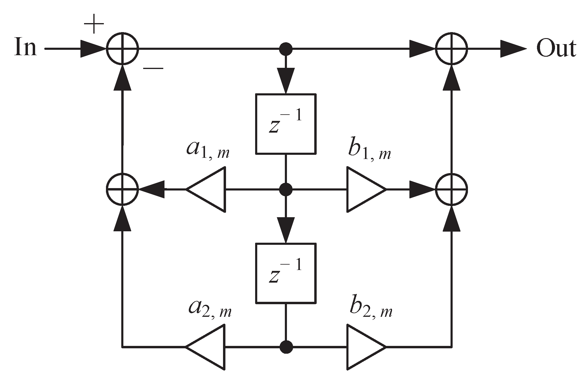
31]. The transfer function of the resulting second-order band filter, implemented with the structure in Figure 2, is:
H m ( z ) = k 0 , m 1 + b 1 , m z 1 + b 2 , m z 2 1 + a 1 , m z 1 + a 2 , m z 2 ,
where m = 1 , 2 , , M . For the third-octave design M = 31 , and for the Bark design M = 24 . The filter coefficients are calculated as:
k 0 , m = V ( G Nq , m + W 2 + A 2 ) ,
b 1 , m = 2 G Nq , m W 2 G Nq , m + W 2 + A 2 ,
b 2 , m = G Nq , m + W 2 A 2 G Nq , m + W 2 + A 2 ,
a 1 , m = 2 V ( 1 W 2 ) ,
a 2 , m = V ( 1 + W 2 A 1 ) ,
using the following variables:
A 1 = C + D | G m 2 G B , m 2 | , A 2 = G m 2 C + G B , m 2 D | G m 2 G B , m 2 | , W 2 = | G m 2 G Nq , m 2 | | G m 2 1 ] tan ω c , m 2 2 , V = 1 1 + W 2 + A 1 .
The following variables are also used to simplify the above formulas:
C = | G B , m 2 G Nq , m 2 | Ω 2 2 W 2 | G B , m 2 G Nq , m | | G B , m 2 1 | | G m 2 G Nq , m 2 | , D = 2 W 2 | G m 2 G Nq , m | | G m 2 1 | | G m 2 G Nq , m 2 | , Ω = 1 + | G B , m 2 1 | | G B , m 2 G Nq , m 2 | W 2 tan B m 2 ,
where G m is the linear peak gain of the filter, G B , m is the gain of the filter at the bandwidth boundaries, B m = 2 π f B , m / f s is the bandwidth, ω c , m = 2 π f c , m / f s is the center frequency, and  f s = 44.1  kHz is the sampling rate. The linear filter gains G m are obtained by converting the optimized dB gains g m = 20 log ( G m ) to linear gain factors:
G m = 10 g m / 20 .
The Nyquist gain for each band filter was calculated with the help of a sufficiently highly oversampled parametric EQ filter emulating the shape of an analog filter, as proposed in [22]. The sample rate was set to 10 MHz, and the filter gain was evaluated at 22.05 kHz, which was the Nyquist limit f s / 2 at the sample rate of 44.1 kHz. The gain estimated this way was used as the Nyquist gain G Nq , m of the band filter. A polynomial approximation for the dependency of the Nyquist gain could be used to simplify the design of the symmetric band filters [22]. Thus, the oversampling method for the Nyquist gain was used only to determine the required polynomial coefficients.

3.1. Third-Octave GEQ using Symmetric Band Filters

The used third-octave center frequencies (spaced equidistantly on a logarithmic scale starting from 1 kHz in each direction) and the optimized bandwidths leading to the best overall performance of the GEQ are shown in Table 1. The nominal bandwidths for the proposed third-octave equalizer were obtained with B m = ( 2 3 1 / 2 3 ) ω c , m 0.4662 ω c , m so that the boundaries of the bands coincided with the center frequencies of the neighboring bands. However, the bandwidths marked with an asterisk in Table 1 were modified from the nominal values in order to account for the frequency warping near the Nyquist limit. The modifications resulted in optimized bandwidths with regard to target magnitude shapes obtained with oversampling. The resulting band filter shapes are seen in Figure 4a, where the squares indicate the gain at the bandwidth boundaries as specified by the parameter c.
Appropriate parameter values must be selected for the WLS design to be accurate. These are the number of iterations, the prototype gain used to obtain the initial interaction matrix B , the parameter c defining the gain at the bandwidth boundaries, and the weighting factors for each band [3,6,22]. The value for each of these parameters was chosen jointly with an optimization loop in MATLAB. For the optimization, 8192 command gain configurations were applied: half of these were random extreme gain settings with each command gain being zero or ±12 dB, and the other half were random settings, where the command gains were integers in the range [−12 12]. Different parameter combinations were used to design a GEQ for each command gain configuration, and the maximum approximation error was calculated (see Section 5 for the error definition). Next, the maximum value and the mean of the maximum errors were computed for each setting combination, as also the number of cases where the error exceeded the allowed error of ±1 dB. Finally, the optimal parameter values were selected based on the best obtained results, giving more weight to the random integer cases than to the extreme command gain configuration.
Based on the parameter optimization, the number of iterations was set to one; the prototype gain was set to 11 dB; the band-boundary parameter was set to c = 0.38 ; but no weighting factors were used, i.e., the weight for all bands was one. The value for the parameter c was reduced slightly compared to the third-octave GEQ in [3], which resulted in narrower peak filters. The widths of the filters were a compromise between their ability to produce flat regions in their magnitude response and, on the other hand, large gain changes between neighboring bands. The prototype gain was used to calculate the initial interaction matrix, and since the prototype gain was predefined, the initial interaction matrix could be calculated beforehand and stored [6].
The value of the prototype gain was not as crucial here as, for example, in [22], where no iterative step was used. Due to the iterative step, where a new interaction matrix was determined based on the first set of optimized filter gains, the initial WLS solution could be seen as a frequency-dependent, improved prototype gain vector. The first iterative step had the biggest effect on the optimized gains [3], and thus, it was useful in improving the accuracy of the GEQ. However, during the optimization, further iterative steps, while improving the accuracy in certain cases, actually decreased the accuracy overall. This might be because there were only 61 design points in the entire audible frequency range, in which case, the WLS solution optimized these points while simultaneously neglecting the frequency areas between them.
For the third-octave design, the magnitude response of the first 22 band filters always stayed at approximately 0 dB at the Nyquist limit, whereas the remaining band filters benefited from adjusting the gain G Nq , m as a function of the peak gain G m , as seen in Figure 5a. The polynomial approximation utilized third-order polynomials for bands m = 23 , 24 , , 31 :
g Nq , m = q 0 , m + q 1 , m g m + q 2 , m g m 2 + q 3 , m g m 3 .
The polynomial coefficients q m , obtained for each band filter using curve fitting in MATLAB, are shown in Table 2. This way, the peak dB gain g m was the only parameter that had to be provided when designing the band filters for the SGE3 design. Note that the coefficients q 0 and q 2 were always zero, since the values given by the curve fitting were so small that they could be rounded to zero. The polynomial approximation produced accurate results compared to the targets shown in Figure 5a, with the maximum error being ± 0.5  dB for the 31st band and less than ± 0.2  dB for the other bands.

3.2. Bark Band Equalizer

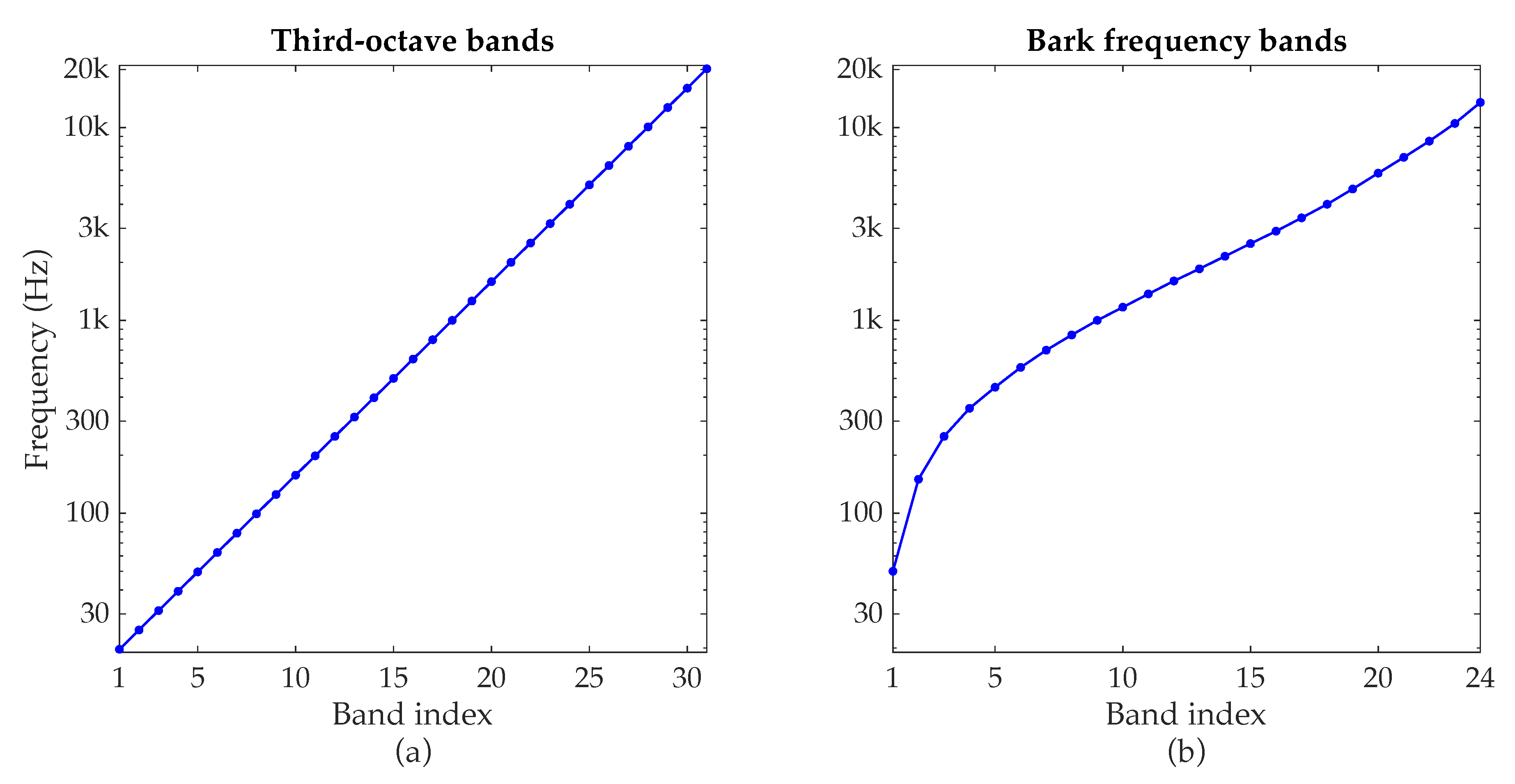
This section tackles the design of a GEQ with a Bark frequency division of bands using symmetric band filters. The design principles were primarily the same as in the third-octave design above, with a few modifications. The main challenge of the Bark GEQ design was the fact that the Bark center frequencies were not equidistantly spaced on the logarithmic frequency scale, as was the case with octave and third-octave designs. Figure 6 illustrates this difference by showing the center frequency of each band on a logarithmic frequency scale. Figure 6a shows that the third-octave center frequencies were located on a straight line, whereas in Figure 6b, the Bark center frequencies formed a nonlinear curve. The numerical data for these plots are given in Table 1 and Table 3.
In addition to the Bark center frequencies, Table 3 gives the bandwidths selected for the band filters. Note that while the center frequencies were selected according to the standard definition [23], the bandwidths were not. This was due to the nature of the least-squares GEQ design: by choosing the bandwidths in Table 3, the user could control the GEQ at the Bark center frequencies to obtain greater overall accuracy. For best accuracy, the band filter’s right bandwidth boundaries had to coincide with the center frequency of the adjacent band filter. This was achieved by setting the bandwidths of the first 23 bands to B m = ω c , m + 1 ( ω c , m 2 ) / ( ω c , m + 1 ) . Since this method could not be applied to the last band filter, its left edge was matched with the center frequency of the penultimate band filter. The resulting band filter responses are shown in Figure 4b.
The Bark EQ design utilized the same filters as the third-octave EQ, and thus, the values for the same parameters had to be optimally chosen. Since the uneven spacing of the Bark center frequencies required the band filters of the GEQ to have different bandwidths, a consequent implication was that the parameter c had to be frequency dependent. Additionally, this complication led to more iteration rounds, a different initial prototype gain, and a non-constant weighting matrix for good accuracy. The parameter optimization was performed in the same way as in the third-octave case above. The only difference was that instead of 4096 random extreme cases (command gains at zero or ±12 dB), only 2048 such gain configurations were used since the results from the random integer gain configurations were eventually emphasized.
Based on the optimization, the parameter c was set to c = 0.36 for the first band and to c = 0.42 for bands 2–24. This way, the leakage of the relatively wide first band filter to its neighboring bands was better controlled. An additional step to improve the accuracy of the Bark GEQ at low frequencies applied frequency-dependent weighting values to the WLS solution. The best accuracy, from among the many choices tested, was achieved when the weighting matrix in (3) was:
W = diag ( 1 0.5 0.5 0.5 ) .
Finally, the Bark EQ design used two iteration steps. The initial interaction matrix was first constructed with a prototype gain of 1 dB, after which (3) was calculated thrice: the interaction matrix for the second and third iteration rounds was obtained using the optimized gains from the first and second WLS solution, respectively. The final solution yielded the optimized band filter dB gains that were then converted to linear gain factors that were used to update the band filter coefficients.
Similarly to the third-octave case, the filter design required the Nyquist gain. In order to have the filter peak gain as the sole input (since the center frequencies and bandwidths were set constants), the Nyquist gain was again approximated with a third-order polynomial based on the peak gain (see (16)). Excessively oversampled versions of the Bark band filters were designed, and their responses were evaluated at 22.05 kHz in order to obtain the necessary data for MATLAB’s curve fitting tool. The Nyquist gains of the first 18 bands were observed to be always approximately zero and thus did not need to be changed. The Nyquist gain relative to the peak gain of bands 19–24, however, were approximated: their target shapes are shown in Figure 5b, and the corresponding polynomial coefficients are given in Table 4. Note that similarly to the third-octave case, coefficients q 0 and q 2 were zero for all filters. For the Bark EQ, the polynomial approximation of the Nyquist gains was highly accurate with the error being less than ± 0.2  dB for all bands in comparison to the target curves in Figure 5b.

3.3. Phase Properties

In order to study the phase properties of the third-octave and Bark band GEQs, an example gain configuration where every slider was set to 12 dB was used for both designs. The resulting magnitude responses are seen in Figure 7. The plots depict the overall magnitude response and the individual band filter responses. The EQs were then used to filter an impulse in order to obtain their impulse responses, which are shown in Figure 8 plotted on the dB scale. The third-octave design produced a much longer impulse than the Bark design. Finally, the group delay of the two EQs was calculated, and the results are presented in Figure 9. Due to the high number of sharp low-frequency filters in the third-octave design, the resulting group delay amounted to over 30 ms at low frequencies. In comparison, the Bark EQ, which employed much wider filters at low frequencies, produced a maximum group delay value of approximately 3.5 ms.

4. Proposed Neural Networks for GEQ Design

This section introduces the proposed neural networks used to simplify and speed up the EQ filter gain optimization of SGE3 and SGEB. The neurally-controlled versions of these GEQs are called NSGE3 and NSGEB, respectively. A network structure (M-2M-M-M) similar to that utilized in the previous work [20] was used for the NSGE3 and NSGEB designs, shown in Figure 3, where each layer size was determined based on the number of EQ filters M. For the third-octave design NSGE3, the network structure was 31-62-31-31, and for the Bark design NSGEB, it was 24-48-24-24. Both neural networks were trained as before in [20] by using MATLAB’s fitnet function with a Bayesian regularization backpropagation algorithm [29].
The benefit of Bayesian regularization is that, in addition to minimizing the mean squared error, it also simultaneously minimizes the network weights, thus preventing overfitting and ensuring good generalization to new data. With Bayesian regularization, the network training should not stop until the neural network converges. A large value of the Levenberg–Marquardt parameter μ [30] is a good indicator of convergence. Thus, the other stopping conditions, such as the number of epochs and the performance goal (MSE error), were set to a high and a low value, respectively, so that the training of the network did not stop before converging. The maximum number of epochs was set to 10,000 and the performance goal to 0.0001. These values were never attained during the training.

4.1. Training the Neural Network for the Third-Octave GEQ Design (NSGE3)

The training dataset for NSGE3 was created with the novel SGE3 least-squares gain optimization technique proposed in the previous section. A total of 1500 input-output gains were created, where seven pairs consisting of extreme cases—all zeros, all up to +12 dB, and zigzag cases—were set manually, while the remaining 1493 input-output pairs were randomized automatically. Essentially, the input gains of the training data were the same as those used in [20], and the output gains were recalculated using the SGE3 method.
The actual training of NSGE3 was conducted in several steps. Since the structure and operation of the NGEQ3 neural network [20] was similar to that of the new NSGE3, the NSGE3 was trained based on the previous network in order to save time in the training. The NGEQ3 neural network was retrained using a training dataset with the same input gains as previously, but where the output gains were calculated using the SGE3 algorithm. The resulting neural network already provided accurate predictions of the optimized filter gain values. After the initial training, the SGE3 routine was further optimized to produce even more accurate results, after which the network was retrained using yet another set of training data, consisting of the same inputs, but updated output gains from the optimized SGE3. The second round of training also converged and turned out to be even more accurate than the first version of the neural network. The accuracy of both proposed methods, SGE3 and NSGE3, is discussed in Section 5.1.

4.2. Training the Neural Network for the Bark GEQ Design (NSGEB)

The neurally-controlled Bark band equalizer NSGEB was trained according to the same principles as NSGE3. This time, there were no earlier models available, so the training of the network had to start from scratch. Furthermore, due to the larger number of EQ bands, the prior training data could not be used, and so, the training data had to be created as well. The new training data included the seven special cases and 1493 random input-output gain pairs for the 24 Bark EQ filters, 1500 cases in total. This dataset was used to train the first version of the NSGEB.
After successful convergence of the training algorithm, the network performance was validated, and it was discovered that although the performance error was reasonable, the network gain prediction did not achieve the largest individual filter gain values accurately enough. Note that although the user-set command gain values were limited to ±12 dB, the actual EQ filter gains could have values larger than 30 dB with certain command gain settings. Thus, a new training dataset was created containing 48 extreme command gain settings that produced EQ filter gains greater than 30 dB on some EQ bands. These extreme cases consisted of command gain values of −12 dB, 0 dB, and 12 dB. Additionally, a new set of random gain input-output pairs was created, so that the total number of data pairs was 1500.
The first version of the neural network was retrained using the second training dataset, which, after convergence, was more accurate than before. This neural network was chosen to be the one used in NSGEB. The performance of SGEB and NSGEB methods is evaluated in the next section.

5. Results

This section compares the accuracy of the proposed designs with previous methods, when applicable. Furthermore, the computing time required to calculate the optimized EQ filter gains and to update the band filter coefficients is evaluated for all proposed designs. The error, with which the accuracy was evaluated in this work, was defined in the same way as in [22]. That is, the maximum of the absolute difference between the user-set command gains and the magnitude response of the GEQ at the command frequencies was evaluated. Additionally, the maximum error was evaluated in the frequency range between any two adjacent command gains when their command gain values were the same. The error was evaluated this way because the target magnitude response was not well defined between command frequencies, and thus, evaluating the error in those regions became cumbersome and controversial. Furthermore, the magnitude response, being composed of the responses of cascaded second-order filters, could be assumed to change monotonically between command points. Furthermore, when two adjacent command gains had the same value, the target gain could be naturally assumed to be constant between the points, with minimal undulation [3].

5.1. Accuracy: SGE3 and NSGE3

The neural network trained to predict the filter gains of the previous third-order GEQ design, called NGEQ3, produced a maximum error of 0.29 dB and a mean maximum error of 0.07 dB in predicting the filter gains [20]. The mean maximum error corresponded to the average of maximum errors computed from many random gain settings. In this case, it was computed using a test set of 10,000 random gain settings, each having 31 pairs of command gains and filter gains. The mean maximum error better described the typical behavior of the GEQ design than the maximum error that only occurred in one particular test setting, usually a very strange one, which may not ever be used in practice. In this case, the accuracy had to be interpreted so that the maximum error caused by the neural network never (according to our wide tests) exceeded 0.29 dB, and it was very likely to be about 0.07 dB in practice. The maximum error of the proposed NSGE3 design was 0.33 dB, and the mean maximum error was 0.07 dB. In comparison to the accuracy of the NGEQ3 method above, these errors were almost the same.
Surprisingly, our tests indicated that the error in the filter gain prediction did not increase the magnitude-response error as much, since the error in the gain value could actually move the magnitude response closer to the command point or the gain prediction error might occur at a frequency where the magnitude-response error was minimal to begin with. Table 5 shows the maximum and mean maximum errors obtained with different design methods: the ACGE3 method had a maximum error of 0.97 dB, and the NGEQ3 method had a max error of 1.05 dB. Thus, the increase in error was only 0.08 dB (compare the maximum errors on the first two lines of Table 5), although the neural network could increase the error in the gain of a single band by as much as 0.29 dB. Similarly, the NSGE3 method was only 0.05 dB less accurate than the SGE3 method (see the last two maximum errors in Table 5), although the maximum error of individual filter gains could be as large as 0.33 dB. Table 5 also shows that the mean maximum error of the proposed NSGE3 method was 0.50 dB, which was slightly better than that of the previous NGEQ3 method, which was 0.54 dB. Furthermore, the maximum errors of both of the proposed designs, SGE3 and NSGE3, were smaller than that of the ACGE3 least-squares design, which was the earlier state-of-the-art method.
Figure 10, Figure 11, Figure 12 and Figure 13 plot the magnitude responses obtained with SGE3 (- -) and NSGE3 () for different illustrative command gain settings (), along with their calculated EQ filter gain values (□ and ×). Ideally, the filter gains predicted by the neural network depicted by green crosses should lie exactly inside the black boxes representing the optimized gains, leading to identical magnitude responses. The title of each figure exposes the largest magnitude error occurring for both SGE3 and NSGE3 at command point frequencies, as described above.
Figure 10 shows a particular test case from the validation dataset in which SGE3 had its largest error of 0.81 dB (see Table 5, Row 3, Column 2). Here, the error occurred at 16,443 Hz, which was between the two highest command frequencies that had the same gain setting of +12 dB. The largest error of NSGE3 was, in this case, slightly smaller (0.75 dB) than that of SGE3, and it occurred at the same frequency. Furthermore, the neurally-controlled filter gains (×) matched closely those optimized using the WLS algorithm (□).
The largest error within the validation dataset for NSGE3 was 0.86 (see Table 5, last row, second column). This case is shown in Figure 11. The error occurred again between adjacent command points, this time at 10,453 Hz, having the same gain value of 12 dB. In this particular case, SGE3 had an error of 0.77 dB, which occurred at the same frequency. Note that the largest errors of the validation set for SGE3 and NSGE3 did not occur with the same command gain settings (see Figure 10 and Figure 11). However, both of the cases had similar local setting of the command gains, where two adjacent high-frequency commands had the same value of +12 dB, and the command gain prior to these had a low negative value, creating a steep slope in the magnitude response. Furthermore, both errors occurred between these two command gain points instead of at the command gain frequency.
Figure 12 shows a zigzag command gain setting, where the command gains altered between ±12 dB, which is known to be difficult for GEQs. Despite this fact, the errors were only about 0.4 dB at the 20-Hz command point. This setting also demonstrated well how different the optimized filter gains (□ and ×) could be from the user-set command gains (), in order to create the magnitude response the user actually wants.
Figure 13 shows a design example with a randomized set of command gains, which illustrates, in a way, a more typical use of command gains compared to the previous extreme cases, shown in Figure 10, Figure 11 and Figure 12. Even with this rather extreme random command gain setting, both SGE3 and NSGE3 performed well with maximum magnitude errors of 0.38 dB and 0.36 dB, respectively, at the 31 Hz command frequency.
Based on the example designs shown in Figure 10, Figure 11, Figure 12 and Figure 13, both SGE3 and NSGE3 performed very accurately. Furthermore, the neural network performed well in all of the example design cases; even when the error was at its largest, the calculated filter gains were close to those of SGE3, which was used to train the network.

5.2. Accuracy: SGEB and NSGEB

The accuracy of SGEB and NSGEB was analyzed similarly to SGE3 and NSGE3 in the previous section. This time, there was really no prior state-of-the-art to make comparisons, since this was the first Bark based GEQ with one second-order filter per band of which the authors knew. Of course, these results could be compared to those of SGE3 and NSGE3. However, the underlying nature of Bark bands led to some difficulties in the GEQ design, as discussed in Section 3.2. Therefore, the errors could be assumed to be slightly larger than those of the SGE3 and NSGE3 designs, which had their command points evenly spaced on the logarithmic frequency scale.
Table 6 shows the results of the magnitude-response accuracy experiment when using a validation dataset of 10,000 random command gain settings, with the same error criteria as was used with the third-octave case before. Table 6 shows the maximum error and the mean of 10,000 error maxima for SGEB and NSGEB. The maximum error was seen to be approximately 1.3 dB for both methods, whereas the mean performance error was about 0.6 dB. In fact, the trained neural network could estimate the filter gains in the validation dataset with high accuracy, which produced magnitude errors that were only 0.06 dB (maximum) and 0.01 dB (mean maximum) larger than the WLS-optimized filter gains used to train the neural network.
Figure 14, Figure 15 and Figure 16 illustrate the performance of the proposed Bark based GEQs via the magnitude responses of SGEB (- -) and NSGEB () and the optimized EQ filter gains (□ and ×) that were calculated based on the user-set command gains (). Figure 14 shows the command gain settings that produced the largest error from the entire validation dataset. This time, the same command gain settings caused the largest errors for both SGEB and NSGEB, which were 1.26 and 1.32 dB, respectively. The largest errors occurred between the second and third command gain frequencies at 157 Hz, when their command gains were set to +12 dB. These types of command gain settings at the lowest command points seemed to cause the maximum errors with the Bark based GEQs. This was due to the wider spread of the low-frequency bands in Bark configuration. In comparison, the third-octave design had 11 filters below 200 Hz, whereas the Bark design had only two.
Despite the challenges caused by the Bark band definition, SGEB and NSGEB could handle even the zigzag case (see Figure 15). The largest error for both designs, around 0.8 dB, occurred at the first command gain frequency of 50 Hz. As can be seen, the magnitude responses extended to all of the other command points well, and the neural network used in NSGEB could predict the band-filter gains with high precision. Moreover, using this example, one can easily see that the Bark bands were not equidistantly placed in the logarithmic domain, when the symmetry of command gains, as well as the filter gains in Figure 12 is compared to that in Figure 15.
Finally, Figure 16 shows a design example with randomized command gains, where the error was close to the mean maximum values shown in Table 6. Here, NSGEB performed slightly better than SGEB with an error of 0.57 dB as compared to 0.62 dB. This time, the errors occurred at the high frequency of 10.5 kHz, implying that the low-end of SGEB and NSGEB operated well.

5.3. Computing Speed

The computing times required to design the band filters were analyzed using MATLAB. The results were an average of computing the filter gains and coefficients for 100,000 random command gain settings. Table 7 shows the results obtained by using a 15 inch MacBook Pro (2017) computer with a 2.8 GHz Intel Core i7. The computing times are presented so that the gain optimization and coefficient update are separated, because the neural networks replaced the gain optimization, whereas the filter coefficients were calculated and updated independently of the gain optimization algorithm. Furthermore, the computing times of the third-octave and Bark GEQs should not be directly compared with each other, because they had a different number of band filters, and the latter design needed more iterations.
Table 7 shows that the least-squares methods, SGE3 and SGEB, required 408 μ s and 526 μ s, respectively, to calculate the optimized gains, whereas the calculation of the filter coefficients took 126 μ s and 101 μ s, respectively. Although SGEB had only 24 EQ filters compared to the 31 EQ filters used in SGE3, the gain optimization was slightly slower, since it used two rounds of iterations in the design, compared to only one iteration in SGE3. However, the filter coefficient update was faster in SGEB than in SGE3, since it was done in the same way in both designs and the Bark band GEQ had fewer filters.
As can be seen from Table 7, the gain calculation time with the neural networks was superior to that of the WLS method. The average gain optimization time was 5.1 μ s for NSGE3 and 4.4 μ s for NSGEB. This meant that the neural-network based third-octave design NSGE3 was approximately 80 times faster than the original SGE3 method, whereas the neural network based Bark design NSGEB was up to 120 times faster than SGEB.

6. Conclusions

This paper introduced an improved cascade design for auditory graphic equalizers having either a third-octave or a Bark band division. Each band was assigned a single second-order IIR section having a symmetric magnitude response and a controllable Nyquist-limit gain. When a logarithmic band division was used, such as in the third-octave case, the band filters with adjustable gain at the bandwidth boundaries allowed strict control of their response at the neighboring band centers. This appeared to be beneficial for accurate GEQ design. Since the Bark frequency division was non-logarithmic, we suggested here that the gain was controlled at the upper boundary of each band filter’s response. The WLS design was applied to solve for the optimal filter gains to account for the interaction between the band filters. The LS optimization was based on an interaction matrix, which was determined with an optimized prototype gain for each band filter. The interaction matrix contained the band filter gains at all center frequencies and their logarithmic mid-points. Since the interaction matrix values varied slightly with filter gain, i.e., the basis functions were nonconstant, an iteration step was needed for the best accuracy. The interaction matrix was updated using the filter gains obtained at the previous iteration.
The resulting maximum magnitude-response error of the proposed third-octave GEQ design called SGE3 was 0.81 dB, which was sufficient even for demanding audio applications. It is often stated that ±1 dB is as much gain error as can be accepted in Hi-Fi audio [2,5,6]. The maximum error of the proposed Bark GEQ design called SGEB was 1.3 dB, indicating that the non-logarithmic frequency division used in the auditory Bark scale was more challenging in terms of filter optimization than the third-octave scale.
Furthermore, we demonstrated how the WLS designs could be replaced with a neural network, as suggested in our previous works for earlier designs [19,20]. A multilayer perceptron with two hidden layers was trained for both GEQs, using 1500 pairs of command gain vectors and corresponding optimized filter gains vectors. In the prediction mode, the perceptron could precisely compute the filter gains for any command gain setting in the range ± 12 dB with a mean accuracy of about 0.5 dB for the third-octave and of about 0.6 dB for the Bark case, whilst considerably speeding up the gain computation. In fact, the trained neural network computed the filter gains 80 times faster than the WLS design method in the third-octave case and about 120 times faster in the Bark case. In addition to speeding up the gain computation, contrary to the WLS based GEQ algorithms, the neural-network approach did not require the GEQ hardware to perform matrix inversions and Fourier transforms in order to solve the LS problem and create the interaction matrix during the iterative step, respectively.
The auditory equalizers described in this work are widely applicable for audio signal processing, such as equalization of loudspeakers, headphones, or sound reproduction systems in rooms. Since the filter design was fully automated and highly accurate, it is perfectly suited to novel intelligent audio applications, such as automatic mixing schemes [32,33], where the graphic equalizer is controlled with artificial intelligence. MATLAB scripts for the proposed GEQ designs are available online at http://research.spa.aalto.fi/publications/papers/applsci-auditoryEQ.

Author Contributions

The contributions to this paper are as follows: conceptualization, J.R., J.L., and V.V.; methodology, J.R. and J.L.; software, J.R. and J.L.; validation, J.R. and J.L.; data curation, J.R. and J.L.; writing, J.R., J.L., and V.V.; visualization, J.R., J.L., and V.V.; supervision, V.V.; funding acquisition, V.V. All authors have read and agreed to the published version of the manuscript.

Funding

The work of Juho Liski was funded in part by the Aalto ELEC Doctoral School. This research is part of the “Nordic Sound and Music Computing Network—NordicSMC”, NordForsk Project Number 86892.

Acknowledgments

The authors would like to thank Luis Costa for proofreading the manuscript.

Conflicts of Interest

The authors declare no conflict of interest. The funders had no role in the design of the study; in the collection, analyses, or interpretation of data; in the writing of the manuscript; nor in the decision to publish the results.

References

  1. Oliver, R.J.; Jot, J.M. Efficient multi-band digital audio graphic equalizer with accurate frequency response control. In Proceedings of the 139th Audio Engineering Society Convention, New York, NY, USA, 29 October–1 November 2015. [Google Scholar]
  2. Välimäki, V.; Reiss, J.D. All about audio equalization: Solutions and frontiers. Appl. Sci. 2016, 6, 129. [Google Scholar] [CrossRef] [Green Version]
  3. Liski, J.; Välimäki, V. The quest for the best graphic equalizer. In Proceedings of the International Conference on Digital Audio Effects (DAFx-17), Edinburgh, UK, 5–9 September 2017; pp. 95–102. [Google Scholar]
  4. Abel, J.S.; Berners, D.P. Filter design using second-order peaking and shelving sections. In Proceedings of the International Computer Music Conference, Miami, FL, USA, 1–6 November 2004. [Google Scholar]
  5. Holters, M.; Zölzer, U. Graphic equalizer design using higher-order recursive filters. In Proceedings of the International Conference on Digital Audio Effects (DAFx-06), Montreal, QC, Canada, 18–20 September 2006; pp. 37–40. [Google Scholar]
  6. Välimäki, V.; Liski, J. Accurate cascade graphic equalizer. IEEE Signal Process. Lett. 2017, 24, 176–180. [Google Scholar] [CrossRef]
  7. Prince, S.; Kumar, K.R.S. A novel Nth-order IIR filter-based graphic equalizer optimized through genetic algorithm for computing filter order. Soft Comput. 2019, 23, 2683–2691. [Google Scholar] [CrossRef]
  8. Tassart, S. Graphical equalization using interpolated filter banks. J. Audio Eng. Soc. 2013, 61, 263–279. [Google Scholar]
  9. Chen, Z.; Geng, G.S.; Yin, F.L.; Hao, J. A pre-distortion based design method for digital audio graphic equalizer. Digit. Signal Process. 2014, 25, 296–302. [Google Scholar] [CrossRef]
  10. Rämö, J.; Välimäki, V.; Bank, B. High-precision parallel graphic equalizer. IEEE/ACM Trans. Audio Speech Lang. Process. 2014, 22, 1894–1904. [Google Scholar] [CrossRef]
  11. Bank, B.; Belloch, J.A.; Välimäki, V. Efficient design of a parallel graphic equalizer. J. Audio Eng. Soc. 2017, 65, 817–825. [Google Scholar] [CrossRef]
  12. Tao, H.; Fang, Y.; Liu, H.; Huang, Q. Optimization method for a high-precision graphic equalizer with lower order filter. In Proceedings of the 14th IEEE International Conference on Signal Processing (ICSP), Beijing, China, 12–16 August 2018; pp. 22–26. [Google Scholar]
  13. Liski, J.; Bank, B.; Smith, J.O.; Välimäki, V. Converting series biquad filters into delayed parallel form: Application to graphic equalizers. IEEE Trans. Signal Process. 2019, 67, 3785–3795. [Google Scholar] [CrossRef]
  14. Karjalainen, M. A new auditory model for the evaluation of sound quality of audio systems. In Proceedings of the IEEE International Conference on Acoustics, Speech, and Signal Processing, Tampa, FL, USA, 26–29 April 1985; pp. 608–611. [Google Scholar]
  15. Patterson, R.D.; Nimmo-Smith, I.; Holdsworth, J.; Rice, P. An efficient auditory filterbank based on the gammatone function. Presented at the meeting of the IOC Speech Group on Auditory Modelling, Malvern, UK, 14–15 December 1987; pp. 1–33. [Google Scholar]
  16. Hohmann, V. Frequency analysis and synthesis using a Gammatone filterbank. Acta Acust. United Acoust. 2002, 88, 433–442. [Google Scholar]
  17. Rämö, J.; Välimäki, V.; Alanko, M.; Tikander, M. Perceptual frequency response simulator for music in noisy environments. In Proceedings of the 45th International AES Conference: Applications of Time-Frequency Processing in Audio, Helsinki, Finland, 1–4 March 2012; pp. 1–10. [Google Scholar]
  18. Johnston, J.D. Transform coding of audio signals using perceptual noise criteria. IEEE J. Sel. Areas Commun. 1988, 6, 314–323. [Google Scholar] [CrossRef] [Green Version]
  19. Välimäki, V.; Rämö, J. Neurally controlled graphic equalizer. IEEE/ACM Trans. Audio Speech Lang. Process. 2019, 21, 2140–2149. [Google Scholar] [CrossRef] [Green Version]
  20. Rämö, J.; Välimäki, V. Neural third-octave graphic equalizer. In Proceedings of the 22nd International Conference on Digital Audio Effects (DAFx-19), Birmingham, UK, 2–6 September 2019; pp. 1–6. [Google Scholar]
  21. Cassidy, R.J.; Smith, J.O. Auditory Filter Bank Lab. Technical Report, Center for Computer Research in Music and Acoustics (CCRMA), and the Department of Electrical Engineering, Stanford University, Stanford, CA, USA. 2008. Available online: https://ccrma.stanford.edu/realsimple/aud_fb/aud_fb.pdf (accessed on 10 February 2020).
  22. Liski, J.; Rämö, J.; Välimäki, V. Graphic equalizer design with symmetric biquad filters. In Proceedings of the IEEE Workshop on Applications of Signal Processing to Audio and Acoustics (WASPAA), New Paltz, NY, USA, 20–23 October 2019; pp. 55–59. [Google Scholar]
  23. Zwicker, E. Subdivision of the audible frequency range into critical bands (frequenzgruppen). J. Acoust. Soc. Am. 1961, 33, 248. [Google Scholar] [CrossRef]
  24. Rämö, J.; Välimäki, V.; Tikander, M. Perceptual headphone equalization for mitigation of ambient noise. In Proceedings of the IEEE International Conference on Acoustics, Speech and Signal Processing (ICASSP), Vancouver, BC, Canada, 26–31 May 2013; pp. 724–728. [Google Scholar]
  25. Välimäki, V.; Franck, A.; Rämö, J.; Gamper, H.; Savioja, L. Assisted listening using a headset: Enhancing audio perception in real, augmented, and virtual environments. IEEE Signal Process. Mag. 2015, 32, 92–99. [Google Scholar] [CrossRef]
  26. Parks, T.W.; Burrus, C.S. Digital Filter Design; John Wiley & Sons, Inc.: New York, NY, USA, 1987. [Google Scholar]
  27. Orfanidis, S.J. Introduction to Signal Processing; Prentice-Hall: Upper Saddle River, NJ, USA, 1996. [Google Scholar]
  28. Smith, J.O. Mathematics of the Discrete Fourier Transform (DFT) with Audio Applications, 2nd ed.; W3K Publishing (online book): Palo Alto, CA, USA, 2008. [Google Scholar]
  29. Foresee, F.D.; Hagan, M.T. Gauss-Newton approximation to Bayesian learning. In Proceedings of the IEEE International Conference on Neural Networks (ICNN’97), Houston, TX, USA, 9–12 June 1997; pp. 1930–1935. [Google Scholar]
  30. Hagan, M.T.; Demuth, H.B.; Beale, M.H.; De Jesús, O. Neural Network Design, 2nd ed.; Martin Hagan: Stillwater, OK, USA, 2014; Available online: http://hagan.okstate.edu/nnd.html (accessed on 10 February 2020).
  31. Orfanidis, S.J. Digital parametric equalizer design with prescribed Nyquist-frequency gain. J. Audio Eng. Soc. 1997, 45, 444–455. [Google Scholar]
  32. Perez-Gonzalez, E.; Reiss, J. Automatic equalization of multichannel audio using cross-adaptive methods. In Proceedings of the 127th Audio Engineering Society Convention, New York, NY, USA, 16–19 October 2009. [Google Scholar]
  33. De Man, B.; Reiss, J.D.; Stables, R. Ten years of automatic mixing. In Proceedings of the 3rd Workshop on Intelligent Music Production, Salford, UK, 15 September 2017. [Google Scholar]
Figure 1. Block diagram of the cascade digital graphic equalizer (GEQ) structure having a single gain term G 0 showing the adjustable filter gains G m .
Applsci 10 01222 g001
Figure 2. Block diagram of a second-order band filter H m ( z ) .
Applsci 10 01222 g002
Figure 3. Neural network structure having two hidden layers. The input parameters g c , 1 , g c , 2 , ..., g c , M are the user-set command gains in dB; the output parameters g o , 1 , g o , 2 , , g o , M are the calculated EQ filter gains in dB; and M is the number of both the command gains and the filter gains. There are M = 31 input and output parameters in the third-octave and M = 24 parameters in the Bark band GEQ.
Applsci 10 01222 g003
Figure 4. All the band filters for the (a) third-octave and (b) Bark cases. The squares indicate the frequency points used to optimize the bandwidths. Note that not all filters are zero at the Nyquist frequency due to the symmetric band filter design.
Applsci 10 01222 g004
Figure 5. Nyquist gain of the different band filters as a function of the peak gain for the (a) third-octave and (b) Bark band case. All curves are antisymmetric with respect to the 0 dB peak gain.
Applsci 10 01222 g005
Figure 6. (a) Third-octave center frequencies vs. (b) Bark center frequencies.
Applsci 10 01222 g006
Figure 7. Magnitude response and individual band filter responses of the (a) third-octave EQ and (b) Bark EQ, when all the command gains are set to 12 dB.
Applsci 10 01222 g007
Figure 8. Impulse response of (a) the third-octave EQ and (b) the Bark EQ corresponding to the magnitude responses in Figure 7.
Applsci 10 01222 g008
Figure 9. Group delays of (a) the third-octave GEQ and (b) the Bark GEQ corresponding to the magnitude responses shown in Figure 7.
Applsci 10 01222 g009
Figure 10. Example design using the proposed SGE3 and NSGE3 methods. With these command gains, SGE3 has its largest error of the entire validation set occurring between two high-frequency command points, 16 kHz and 20 kHz, which have the same command gain of 12 dB. The largest error of NSGE3, in this case, is smaller than that of SGE3.
Applsci 10 01222 g010
Figure 11. Example design using the proposed SGE3 and NSGE3 methods. With these command gain settings, included in a random set of 10,000 configurations, NSGE3 has its largest error of the entire validation set occurring between the two highest command points 10 kHz and 12.7 Hz, which have the same command gain of 12 dB.
Applsci 10 01222 g011
Figure 12. The ± 12 dB zigzag test on third-octave bands using the proposed SGE3 and NSGE3 methods. Now, the largest magnitude-response error for both methods occurred at the 20 Hz command point.
Applsci 10 01222 g012
Figure 13. Example design using the proposed SGE3 and NSGE3 methods showing a typical result with a random command gain configuration in third-octave bands.
Applsci 10 01222 g013
Figure 14. Example design using the proposed SGEB and NSGEB methods showing the largest errors for the entire validation dataset for both Bark band designs. The largest errors occurred at 157 Hz, between the second and third command points.
Applsci 10 01222 g014
Figure 15. Zigzag test, similar to Figure 12, using the proposed SGEB and NSGEB methods. The largest errors occur at the center frequency of the first Bark band at 50 Hz.
Applsci 10 01222 g015
Figure 16. Example design using the SGEB and NSGEB methods showing their typical performance for a randomized command gain setting.
Applsci 10 01222 g016
Table 1. Standard 31 third-octave center frequencies f c and adjusted bandwidths f B used in the proposed symmetric third-octave GEQ.
m f c  (Hz) f B  (Hz)m f c  (Hz) f B  (Hz)m f c  (Hz) f B  (Hz)m f c  (Hz) f B  (Hz)
119.699.1789125.058.2817793.7369.7 *2550402338 *
224.8011.5610157.573.43181000465.8 *2663502943 *
331.2514.5711198.492.51191260586.8 *2780003704 *
439.3718.3612250.0116.6201587739.3 *2810,0804638 *
549.6123.1313315.0146.9212000930.6 *2912,7005684 *
662.5029.1414396.9185.02225201172 *3016,0006803 *
778.7536.7115500.0233.12331751476 *3120,1604117 *
899.2146.2516630.0293.72440001857 *
* Adjusted (reduced) bandwidths due to frequency warping close to the Nyquist limit.
Table 2. Polynomial coefficients for the Nyquist gain of band filters H m ( z ) , m = 23 , 24 , 31 , in the third-octave design.
m2324252627
q 1 , m 0.001660.002950.005440.01050.0214
q 3 , m 8.09 × 10 6 1.25 × 10 5 1.91 × 10 5 2.84 × 10 5 4.08 × 10 5
m28293031
q 1 , m 0.04560.1030.257−0.754
q 3 , m 5.46 × 10 5 6.27 × 10 5 3.68 × 10 5 −1.18 × 10 4
Table 3. Bark center frequencies [23] f c and their adjusted filter bandwidths f B used in the proposed Bark GEQ. Note that these bandwidths used for filter design are different from the standard Bark bandwidth definitions.
m f c  (Hz) f B  (Hz)m f c  (Hz) f B  (Hz)m f c  (Hz) f B  (Hz)
150133.391000315.51734001110
2150160.0101170370.81840001467
3250171.4111370426.91948001828
4350177.8121600466.22058002194
5450214.7131850558.12170002735
6570235.9142150651.02285003619
7700256.7152500744.82310,5005333
8840294.4162900926.52413,5006000
Table 4. Polynomial coefficients for the Nyquist gain of band filters in the Bark equalizer design SGEB.
m192021222324
q 1 , m 0.003770.006060.01110.02440.07140.134
q 3 , m 1.61 × 10 5 2.30 × 10 5 3.43 × 10 5 5.35 × 10 5 7.98 × 10 5 8.37 × 10 5
Table 5. Comparison of magnitude-response accuracy in 10,000 random gain settings: third-octave design. The smallest errors in each column are emphasized.
Design MethodError at Commands Points *
MaxMean Max
ACGE3 [3]0.97 dB0.53 dB
NGEQ3 [20]1.05 dB0.54 dB
SGE3(Proposed, WLS design)0.81 dB0.50 dB
NSGE3 (Proposed, neural network)0.86 dB0.50 dB
* When two neighboring command gains were the same, the error was also measured in the frequency range between the command points.
Table 6. Comparison of the magnitude-response error in 10,000 random gain settings: Bark band design. The smallest error in each column is emphasized.
Design MethodError at Commands Points *
MaxMean Max
SGEB (Iterative WLS design)1.26 dB0.60 dB
NSGEB (Neural network)1.32 dB0.61 dB
* When two neighboring command gains were the same, the error was also measured in the frequency range between the command points.
Table 7. Comparison of computation times required for parameter update in MATLAB. The average of 100,000 test runs is shown in each case. The fastest gain computation times and total times are emphasized.
MethodGainCoefficient
ComputationUpdateTotal
SGE3 (iterative WLS design)408  μ s126  μ s534  μ s
NSGE3 (neural network)5.1  μ s126  μ s131  μ s
SGEB (iterative WLS design)526  μ s101  μ s627  μ s
NSGEB (neural network)4.4  μ s101  μ s105  μ s

