Regressed Terrain Traversability Cost for Autonomous Navigation Based on Image Textures

Abstract

The exploration of remote, unknown, rough environments by autonomous robots strongly depends on the ability of the on-board system to build an accurate predictor of terrain traversability. Terrain traversability prediction can be made more cost efficient by using texture information of 2D images obtained by a monocular camera. In cases where the robot is required to operate on a variety of terrains, it is important to consider that terrains sometimes contain spiky objects that appear as non-uniform in the texture of terrain images. This paper presents an approach to estimate the terrain traversability cost based on terrain non-uniformity detection (TNUD). Terrain images undergo a multiscale analysis to determine whether a terrain is uniform or non-uniform. Terrains are represented using a texture and a motion feature computed from terrain images and acceleration signal, respectively. Both features are then combined to learn independent Gaussian Process (GP) predictors, and consequently, predict vibrations using only image texture features. The proposed approach outperforms conventional methods relying only on image features without utilizing TNUD.

1. Introduction

1.1. Background

The autonomous exploration of unstructured environments by mobile robots is witnessing increased interest, as it helps to accomplish diverse tasks such as search and rescue, surveying and data collection (e.g., [1] with unmanned ground vehicles and [2] with unmanned aerial vehicle), and surveillance. Performing these missions by autonomous mobile robots presents several advantages. It allows the avoidance of human intervention in hazardous area [3], as well as overcomes difficulties that may arise in the case of remotely controlled mobile robots such as a loss of connectivity or degraded latency. With robots being utilized in a wide spectrum of unstructured environments, the need for systems to build reliable representations of the environment is critical. Therefore, the estimation of the traversability of terrains is of great importance. In the so-called model-based approach, traversability is estimated based on mechanical analysis or simulation (e.g., [4,5]). However, the approach requires detailed knowledge of the terrain properties and high computational complexity [6]; hence, it is not easily applicable to certain environments. The other approach, which is becoming more popular, is to rely on machine learning techniques based on many data samples.

While supervised learning methods have proven to be efficient (e.g., [7,8,9]), there are several drawbacks to such methods. Manually labeling a large amount of data to train the classifier is tedious and subject to inconsistency. As a result, this approach is not flexible as it is unable to adapt to dynamic environments without more data annotation and training. As an alternative, self-supervised learning, using proprioceptive sensor information, such as inertial data, as label information to determine whether terrains is traversable, has been intensively investigated [10]. The self-supervised approach, also called the near-to-far strategy [11,12], is promising for making mobile robots adaptive to a variety of environments.

1.2. Related Works on Unsupervised Learning Approaches to Traversability Prediction

As an input for the traversability prediction, LiDAR (either 2D [13] or 3D [9,14]) and stereo camera images [15,16,17] have been widely used. Shape attributes of the ground have been extensively investigated for traversability estimation. The idea is to use 3D environment analysis methods and chart the mobility smoothness in a hierarchical manner. Based on this, 3D Ladar information has been clustered according to scatterness (grass), surfaceness (ground), and linearness (tree trunks) for terrain modeling [18].

Although laser sensors are more precise than stereo cameras, they are still costly and do not necessarily provide sufficient precision due to the sparseness of the 3D points. In particular, they are not perfectly able to detect small unevenness in the terrain in front of a robot despite their high applicability for detecting obstacles with sufficient size and height. Compared with laser sensors, cameras are more affordable and provide different attributes of terrain from 3D geometry obtained through point clouds. Thus, it is important to pursue the availability of image information for the prediction of traversability. In this paper, we investigate the applicability of 2D image features obtained by a camera for traversability prediction.

From the viewpoint of output as a measure of traversability for the self-supervised learning, the discrimination of traversable/non-traversable terrains [10,16] and the classification of terrains, such as gravel/sand/grass [19,20,21,22], are frequently used. One problem of discriminating traversable/non-traversable terrains as the output of the classifier is that the boundary between the two classes is inconsistent and depends on the environment or requirements on the robot. When all regions around a robot are classified as traversable, the robot might still prefer to select a path with minimum (small) damage to its body considering the accumulation of fatigue during a long operational period. In contrast, even if every region around it is classified as non-traversable, the robot might have to search for the least hazardous path to escape from a situation. Thus, the predictability of a continuous cost is more important for avoiding damage to the robot. From the same viewpoint, classifying terrains (gravel/sand/etc.) is not the ultimate goal of traversability prediction; however, cost/damage to the robot should be considered.

As continuous measures of traversability assessment, the slippage of wheels of planetary rovers [6] and the deformability of rocky terrains [11,23] have been investigated. Considering the general use of mobile robots in outdoor environments, however, it is useful to consider not only large-scale unevenness, such as rocky and slippy terrains, but also small-scale unevenness, which causes vibrations or (vertical) acceleration. By considering such small-scale unevenness, it becomes possible to reduce accumulated damage to the robot and instability of its cargo and improve the comfort of passengers.

1.3. Objective and Approach

In this paper, we propose a framework to enable mobile robots to autonomously learn terrain traversability using only their sensors in a self-supervised manner. Terrain traversability is predicted as a cost measured by an acceleration sensor equipped by the mobile robot. Focusing on the usage of image features for terrains with small-scale unevenness, a texture-based prediction of traversability was proposed in [24]. However, the applicability of the texture information in 2D images has not been sufficiently investigated because, in natural environments, terrains are not always uniform and often are non-uniform, therein containing spiky materials such as relatively large stones and roots of trees. This non-uniformity causes traversability cost prediction to be challenging. In this paper, a detection of such non-uniformity in terrains is proposed based on multiscale local image features. It is shown that we can improve the prediction performance prediction performance of the texture-based approach. An advantage of the texture-based approach is that the sensor is affordable and can still detect motion features of the traversing robot without high-cost 3D sensing of the terrain geometry.

To reduce the difficulty of motion feature prediction due to spiky objects in terrains, the classification of images into uniform/non-uniform is introduced. Predictors generated by a Gaussian process [25] are independently applied to uniform/non-uniform terrains so that each predictor can be specialized to learn each type of terrain. The proposed framework for improving the prediction performance is evaluated through comparison with existing texture-based motion feature prediction.

The remainder of the paper is structured as follows. In Section 2, the problem definition is given. Section 3 gives an overview of the system architecture, introduces how terrain uniformity detection is applied, and describes terrain traversability estimation from exteroceptive and proprioceptive information. Section 4 presents the experimental results of the proposed method. Finally, Section 5 concludes this paper.

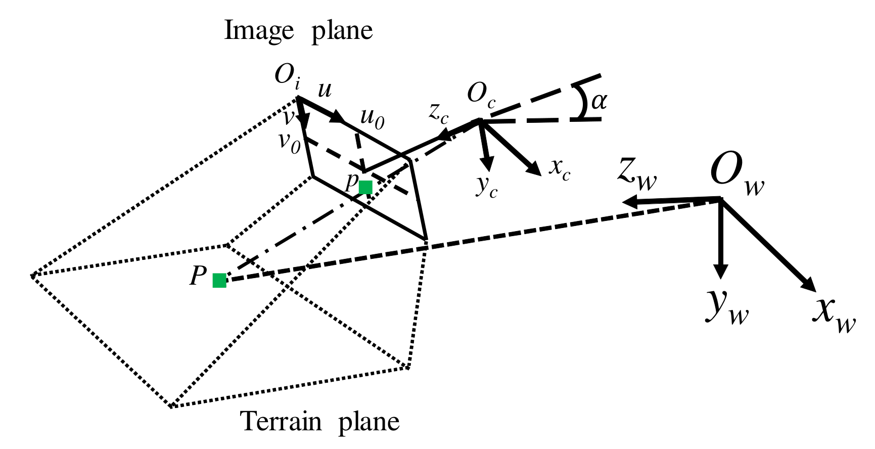
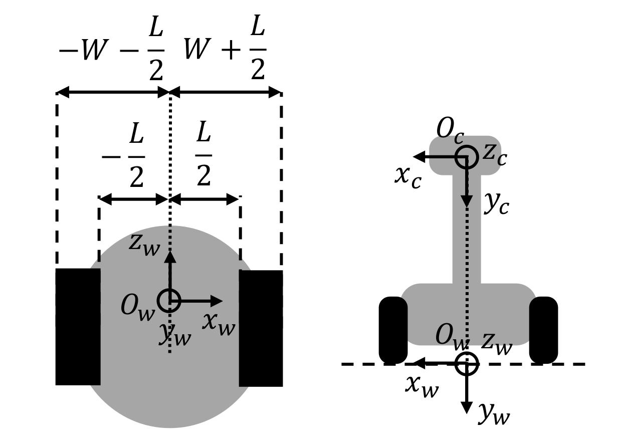
2. Problem Definition

Terrains considered in this study are not always uniform due to irregular obstacles, such as large stones and roots of trees, and are assumed to be traversable even at a higher cost than homogeneous terrains. Typical obstacle size varies between 40 to 80mm in height, which is a significant mobility challenge for the mobile robot as the wheels radius is 105mm. Terrains are assumed to be rigid. Deformable terrains [11] that can lead the mobile robot to lose balance, or cause slippage/sinkage [26], are not covered in this paper. In addition, untraversable terrains are also beyond the scope of this paper. Samples of the terrains investigated in this paper are introduced in Figure 1 and Figure 2.

This study was conducted with a widely used mobile platform (Pioneer 3AT) for navigation and traversability projects in outdoor environments [27,28,29,30]. The platform is driven by four wheels and is capable of traversing bumps up to 100mm, gaps up to 150mm, and slopes up to 19∘. The mobile platform is equipped with a vision sensor and an acceleration sensor, as shown in Figure 3. The camera gathers terrain images, and the IMU registers the acceleration signal generated during a sequence of a run. The goal is to estimate vibrations as a measure of traversability only from terrain images. The predicted traversability cost will be used to anticipate the motion nature of subsequent terrains and is expected to enable a safe run. The focus is not on which robot offers the best handling of terrain unevenness but on enabling any type of robot, regardless of its construction/configuration, to traverse non-uniform terrains.

In the bird’s-eye view given by Figure 4, the gray circle represents the mobile robot and the black rectangles are the wheels. The wheel base and the wheels radius are denoted by L and r respectively. The system accepts as input $v_{\mathrm{l}}$ and $v_{\mathrm{r}}$ as input, respectively, which are the angular velocities of the left and right wheels. The mobile robot motion is described as follows:

$$\left\{\begin{array}{c}z\left(t\right)=\frac{r}{2}\times (v_{\mathrm{l}}\left(t\right)+v_{\mathrm{r}}\left(t\right))\times t\times cos\left(\varphi \left(t\right)\right),\hfill \\ x\left(t\right)=\frac{r}{2}\times (v_{\mathrm{l}}\left(t\right)+v_{\mathrm{r}}\left(t\right))\times t\times sin\left(\varphi \left(t\right)\right),\hfill \\ \varphi \left(t\right)=\frac{r}{L}(v_{\mathrm{l}}\left(t\right)-v_{\mathrm{r}}\left(t\right)),\hfill \end{array}\right.$$

(1)

where x and z are the robot position and $\varphi$ is the orientation of the platform. The angular velocities for both the left and right wheels are similar; therefore, the robot will run straight according to the world $Z_w$-axis. Moreover, the effects of steering and acceleration/deceleration are nonexistent. The mobile robot has no suspension system, that is, it is a rigid body. Hence, effects of interaction of the mobile platform on the right and left wheels will appear on the sensor values. Operating in outdoor environments comes with a very important lightning conditions challenge. To simplify the problem setting, experiments were conducted under fair light conditions with neither shadows nor strong backlight.

3. Traversability Cost Prediction

3.1. Algorithm Architecture–Overview

Using data received from sensors, the mobile robot will build a model of the environment to predict terrain vibrations necessary to enable safe autonomous navigation. The overall system architecture is given in Figure 5. The architecture consists of the sensors available on the robot, which are a mono-vision system, an acceleration sensor, and odometers. The camera is responsible for gathering images of subsequent terrains. The inertial unit measures acceleration signals generated while traversing. The wheel odometer tracks the position of the mobile platform over time. The proposed method follows offline and online processes to achieve traversability cost prediction.

In the offline process, sensor information required for generating the traversability cost predictor is collected. Multiscale analysis measures a low-level image feature that is contrast distance feature to localize irregularities in terrain images. In terrain non-uniformity detection (TNUD), the resulting feature map from the multiscale analysis, is tested to determine whether the terrain nature is homogeneous or non-homogeneous. Region of Interest (ROI) localization extracts image regions traversed by the mobile robot based on its physical features and the camera model. The texture analysis calculates the texture features using the fractal dimension. Using the acceleration signal, the vibration analysis calculates the motion feature. Based on the output of TNUD, image and motion features are used to approximate either the function for uniform or non-uniform terrains.

In the online process, the same steps accomplished in the above mentioned offline process are executed to obtain the terrain image properties, that is, the terrain image properties, texture feature and terrain category. Based on the terrain category class, the vibrations of the subsequent terrain are inferred using texture information and the learned function.

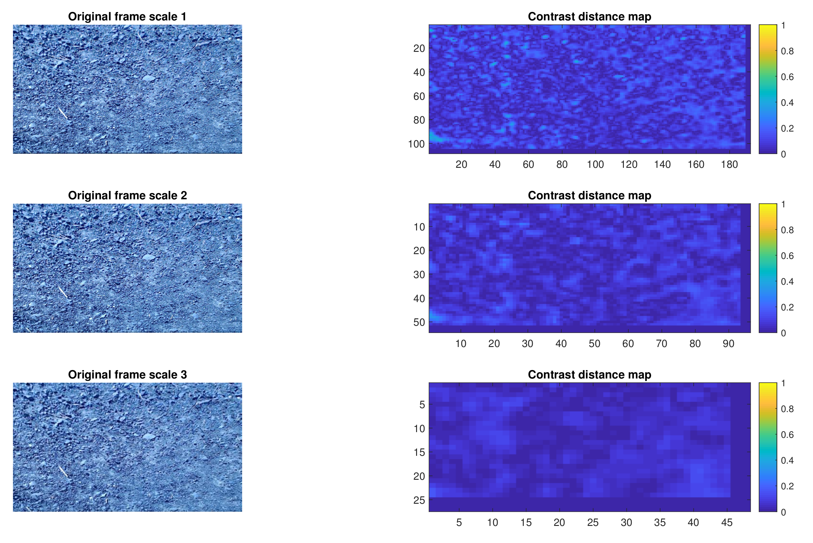
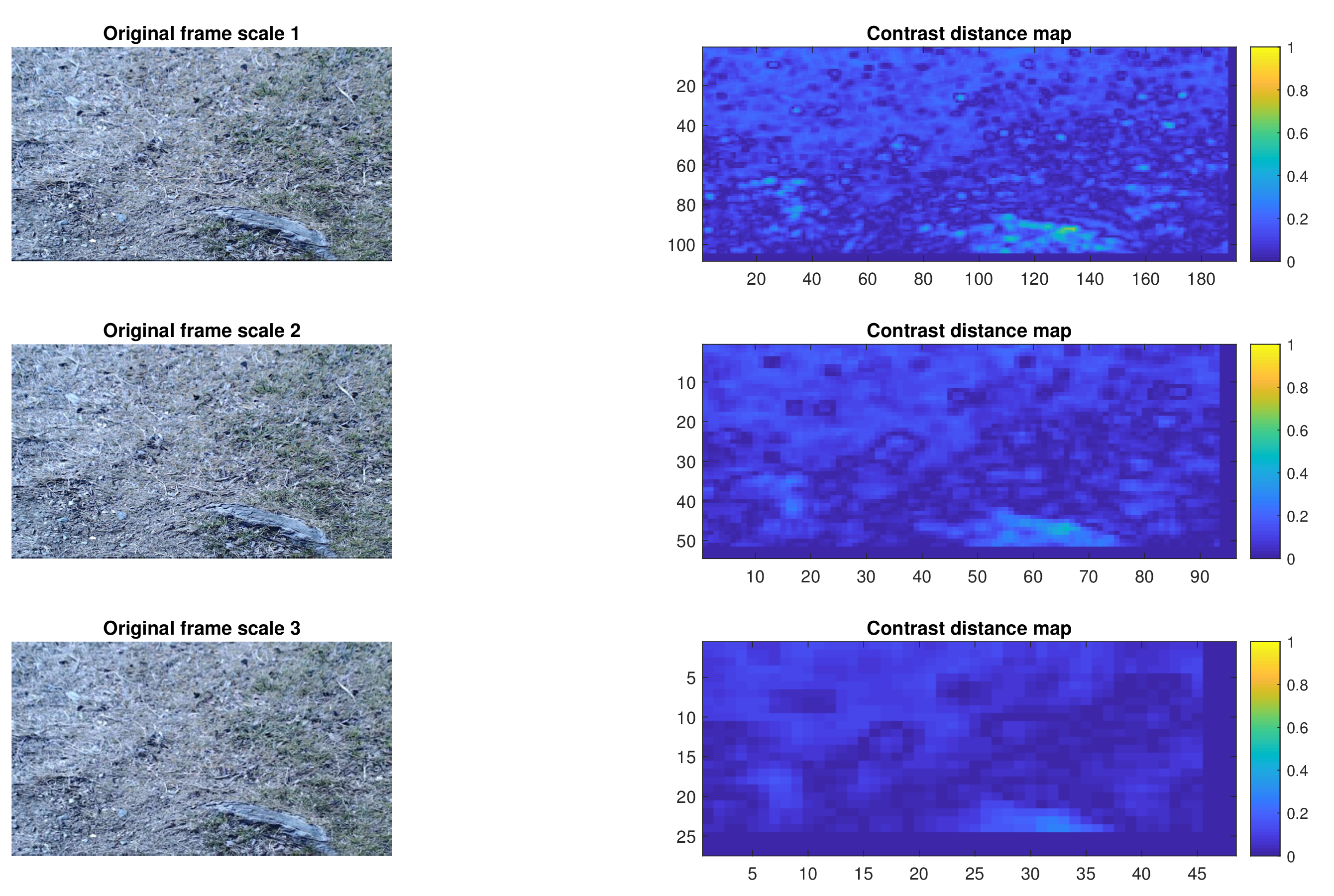
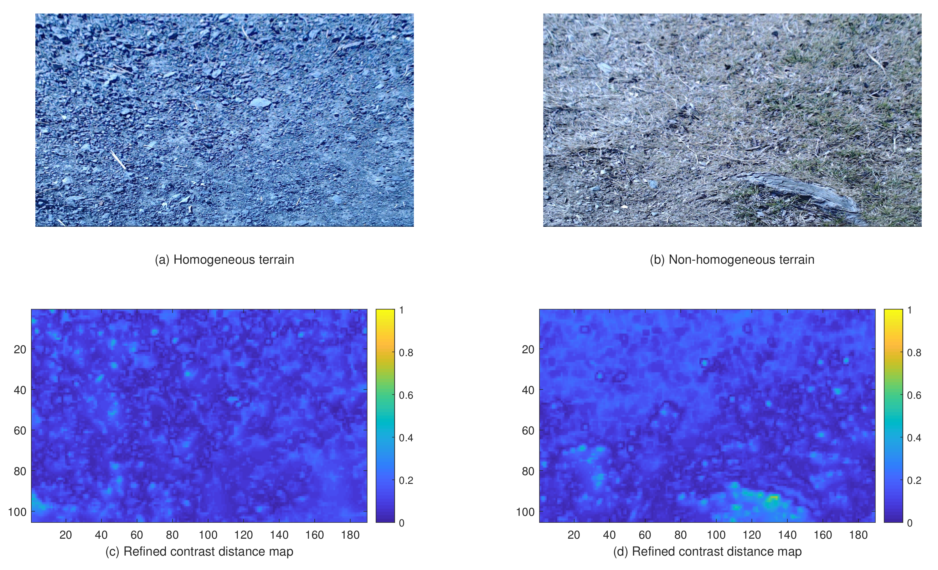
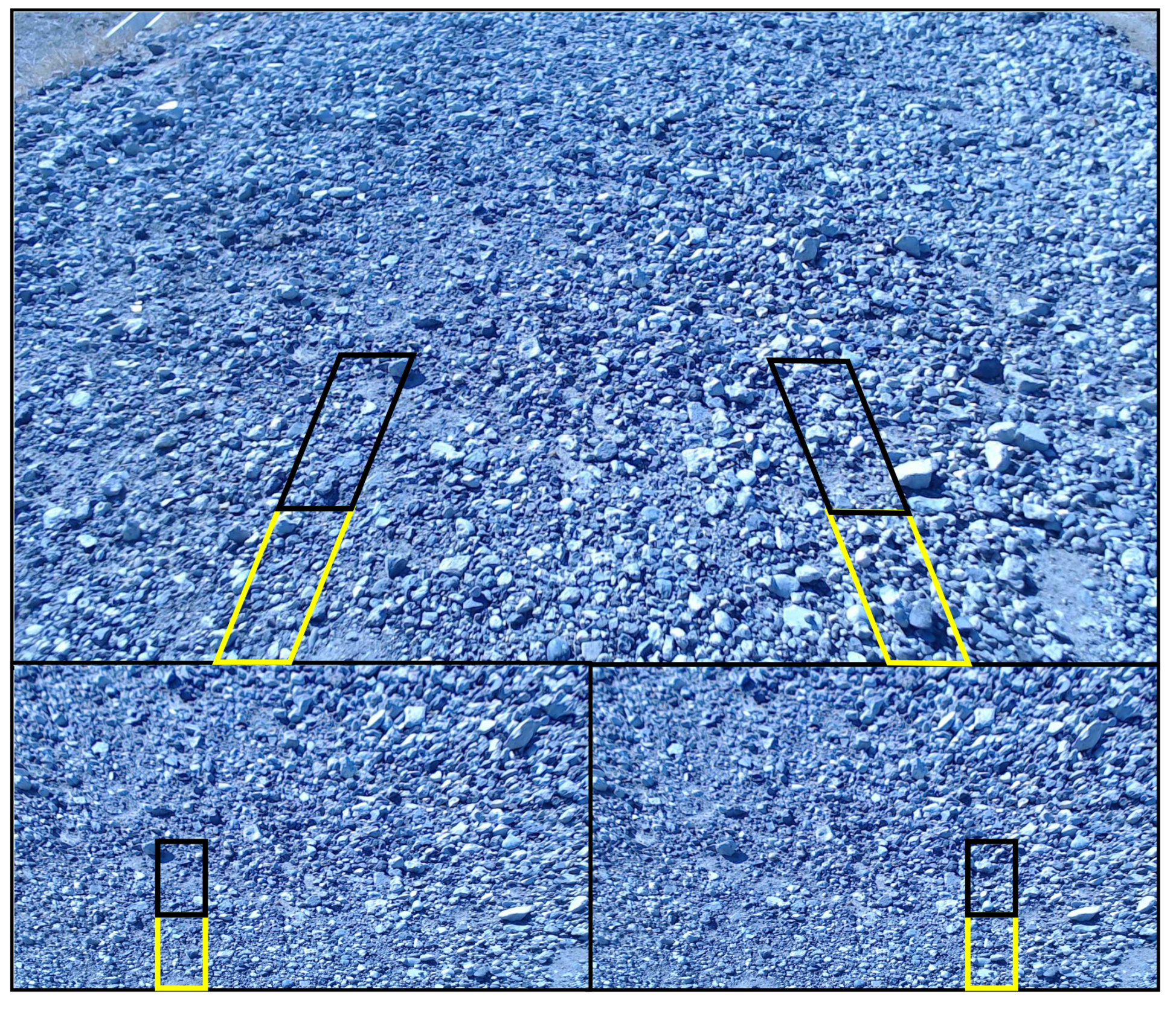
3.2. Terrain Non Uniformity Detection-Region Extraction

Terrain non-uniformity detection aims at identifying whether ahead of the unmanned ground vehicle is a uniformly distributed terrain or contains spiky material. TNUD can be treated as a low-level image processing problem. A bump in a terrain image, as an example of spiky terrain, can be different from the background in terms of contrast. Thus, to detect bumps, we evaluate the lightness contrast distance for each block in the terrain image. Let $\mathbf{I}$ denote the input terrain image. $\mathbf{I}$ is divided into overlapping blocks of size $w\times w$ pixels. Bumps tend to have a higher contrast value than their surrounding regions. Therefore, we measure the distance contrast between the local and global contrast values of the blocks and input image $\mathbf{I}$, respectively. For this purpose, two additional scale images are produced by resizing the original image to half and a quarter by bicubic interpolation. Then, R, G, B values are converted to L*, a*, b* measured in the Commission Internationale de l’ Eclairage (CIE 1976) (L*, a*, b*) color space (CIELAB) as described in [31]. Using the lightness channel, the global lightness contrast of the image is measured by:

$$C\left(\mathbf{I}\right)=STD\left(\mathbf{I}\right)/max\left(MEAN\right(\mathbf{I}),1),$$

(2)

where $STD\left(\mathbf{I}\right)$ and $MEAN\left(\mathbf{I}\right)$ denote the standard deviation and mean values of the input image $\mathbf{I}$, respectively. Let x denote a block in the input image $\mathbf{I}$, and let $C\left(\mathbf{x}\right)$ denote the lightness contrast measured for x. $C\left(\mathbf{x}\right)$ is given as:

$$C\left(\mathbf{x}\right)=STD\left(\mathbf{x}\right)/max\left(MEAN\right(\mathbf{x}),1),$$

(3)

where $STD\left(\mathbf{x}\right)$ and $MEAN\left(\mathbf{x}\right)$ denote the standard deviation and mean values of the block x. The contrast distance is calculated using the results of Equations (2) and (3) as follows:

$$CD\left(\mathbf{x}\right)=∥C\left(\mathbf{I}\right)-C\left(\mathbf{x}\right)∥,$$

(4)

where $CD\left(\mathbf{x}\right)$ denotes the lightness contrast distance value of the block x. Sample results are given in Figure 6 and Figure 7.

To detect non-uniformity in terrain image, all scale maps are combined together to compute a refined contrast distance map using a maximum operator. As shown in Figure 8, non-uniform image regions tend to have a higher contrast distance value than the surrounding uniform areas.

From the terrain images, regions traversed by the mobile robot are considered for texture extraction. For this purpose, the camera model in [32] is employed to define ROIs. As shown in Figure 9, the camera is defined by the camera frame {Oc,xc,yc,zc} where $O_c$ is the center. The following equation projects a point from the world reference frame given by $P\in {\mathbb{R}}^4$ to $p\in {\mathbb{R}}^3$ (both containing one as the last element) onto the image plane:

$$p=\mathbf{K}\left[\mathbf{R}\right|t]P,$$

(5)

where $\left[\mathbf{R}\right|t]\in {\mathbb{R}}^{4\times 4}$ is the extrinsic parameter matrix, and $\mathbf{K}\in {\mathbb{R}}^{4\times 3}$ is the camera parameter matrix obtained through a calibration process.

The above-mentioned model will be combined with the physical characteristics of the UGV, that is, the UGV’s wheels base L and width W to determine the image regions traversed by the mobile robot. As shown in Figure 10, both camera and world reference frames are centered on the platform. The world reference frame is given by {Ow,xw,yw,zw} with $O_w$ as the origin. The objective is to map points to identify the inner and outer bounds of the terrain region crossed by the vehicle. All points belong to the same line; hence, only the depth components with respect to the $w_z$-axis will change. For both the left and right sides, the coordinates of these points are expressed as follows:

$$\left\{\begin{array}{c}{P}_{ro}=[\frac{L}{2}+W,0,z_w]\hfill \\ P_{\mathrm{ri}}=[\frac{L}{2},0,z_w]\hfill \\ P_{\mathrm{lo}}=[-\frac{L}{2}-W,0,z_w]\hfill \\ P_{\mathrm{li}}=[-\frac{L}{2},0,z_w]\hfill \end{array}\right.,$$

(6)

where $P_{\mathrm{ro}}$ and $P_{\mathrm{ri}}$ denote the points laying on the right outer and inner bounds, respectively, and $P_{\mathrm{lo}}$ and $P_{\mathrm{li}}$ denote the left outer and inner bounds. The results of this operation are shown in Figure 11. To increase the number of terrain samples, two terrain patches will be extracted from a single image. The warp perspective transformation is performed to remove the trapezoidal shape introduced when taking a picture.

3.3. Texture and Vibration Features Extraction/Association

In this paper, texture features are obtained using of segmentation-based fractal texture analysis (SFTA) [33]. The SFTA method operates in two steps. In the first step, the input grayscale image is split into binary images using the two-threshold binary decomposition (TTBD) [33]. In the second step, binary images are used to compute the fractal dimension from its region boundaries. TTBD returns a set of thresholds T calculated by the multilevel algorithm [34]. After obtaining the targeted threshold number $n_{\mathrm{t}}$, pairs of contiguous thresholds $T\cup \left\{n_{\mathrm{l}}\right\}$ with $n_{\mathrm{l}}$ being the highest value in the input gray scale image, in combination with pairs of thresholds $\{t,n_{\mathrm{t}}\}$ with $t\in T$, are employed to obtain the binary images as follows

$$I_{x,y}^b=\left\{\begin{array}{cc}1,\hfill & \mathrm{if}{t}_{\mathrm{l}}<I(x,y)\le t_{\mathrm{u}}\hfill \\ 0,\hfill & \mathrm{otherwise}\hfill \end{array}\right.,$$

(7)

where $I_{x,y}^b$ denotes the binary value of image pixel $(x,y)$, $t_{\mathrm{l}}$ and $t_{\mathrm{u}}$ denote the lower and the upper threshold values, respectively. Therefore, $2n_{\mathrm{t}}$ binary images will be obtained. In this paper, the SFTA feature vector includes only the fractal dimension of the boundaries. Let $\Delta (x,y)$ denote the border image of the binary image $I_{x,y}^b$, and which is obtained by the following equation:

$$\Delta (x,y)=\left\{\begin{array}{cc}1,\hfill & \mathrm{if}\exists (x^{\prime },y^{\prime })\in N_{x,y}\hfill \\ \hfill & \mathit{s}.\mathit{t}.I_{x^{\prime },y^{\prime }}^b=0\wedge I_{x,y}^b=1\hfill \\ 0,\hfill & \mathrm{otherwise}\hfill \end{array}\right.,$$

(8)

where $N_{x,y}$ is the 8-connexity of a pixel $(x,y)$. $\Delta (x,y)$ takes on a value of if the pixel at location ($x,y$) in the related binary image $I_{x,y}^b$ has a value of one and has a minimum one neighbor pixel with a value of zero. The border image serves to compute the fractal dimension $D\in \mathbb{R}$ by the box counting method as follows

$$D_0(x,y)=\underset{\epsilon \to 0}{lim}\frac{logN\left(\epsilon \right)}{log\left({\epsilon }^{-1}\right)},$$

(9)

where $N\left(\epsilon \right)$ is the number of hyper-cubes of length $\epsilon$ that fill the object. In this paper, the obtained SFTA feature vector is referred to as $\mathit{x}\in {\mathbb{R}}^{2n_{\mathrm{t}}}$.

Let $a_k,k=1,\cdots ,K$ be the vertical acceleration signal representing vibrations generated from the interaction of the wheels with the terrain when traversing a short range distance, where k is the time step and K is the total time steps. The amplitude distance is retained to describe the behavior of the mobile platform, and is measured by

$$a_{k_{\mathrm{d}}}=\underset{k=1,\cdots ,K}{max}{a}_k-\underset{k=1,\cdots ,K}{min}{a}_k.$$

(10)

According to [35], all motion features (amplitude distance, root mean square, kurtosis, skewness, and crest factor) have a similar level of correlation with the SFTA feature. The amplitude distance feature was chosen as it is easy to implement and to understand. The acceleration signal does not undergo any noise filtering operation, and it is clear whether any filtering is performed at the sensor level. To measure the noise contribution to the measurements, signal-to-noise ratio (SNR) of the acceleration signal at rest was computed as follows:

$$SNR=\frac{\mu }{\sigma },$$

(11)

where $\mu$ and $\sigma$ are the mean and standard deviation of the acceleration signal, respectively. Results of SNR calculation for four signals are given in

Table 1. Signal to noise ratio (SNR) of acceleration signal at rest.

Mean	Standard Deviation	SNR
1.0346	0.0101	102.6474
1.0339	0.0102	101.5350
1.0250	0.0096	106.7354
1.0335	0.0099	104.2580

. SNR values are high which means that the noise does not impact severely our intended purpose.

Two subsequent terrain segments serve for image feature extraction. Appropriately, the relevant acceleration segment for motion feature calculation is paired to the image features by means of the coordinate transformation and odometry. As shown in Figure 12, at time $t=0$, the robot is located at the origin of the world reference frame. The position used to take a new terrain image, denoted here by $Z_{I_i(x,y)}$, is expressed as

$$Z_{I_i(x,y)}=i{d}_s,i=1,\cdots ,N_{\mathrm{image}},$$

(12)

where $d_s$ denotes the sampling distance, and $N_{\mathrm{image}}$ is the total number of terrain images acquired during a run. Due to the camera tilt angle $\alpha$, terrains will be covered from a certain position, expressed as

$$Z_{I_i(x,y)}+Z_{\mathrm{BZ}},i=1,\cdots ,N_{\mathrm{image}},$$

(13)

where $Z_{\mathrm{BZ}}$ is the blind spot. The motive behind focusing on a short distance range l covered by the images for texture feature extraction is that pixels further from the camera focus point are subject to more noise. Thus, visual information may fail to faithfully represent the environment. The acceleration signal sequence generated when traversing a distance l is used for motion feature extraction, and is limited according to the ROI as follows

$$A_i=[Z_{I_i(x,y)}+Z_{\mathrm{BZ}},Z_{I_i(x,y)}+Z_{\mathrm{BZ}}+l],$$

(14)

where $A_i$ denotes the ROI.

3.4. Traversability Cost Regression using Gaussian Process (GP)

The Gaussian process [25] is used for regression analysis. Let $\mathcal{D}=\left\{({\mathit{x}}_j,y_j),j=1,\cdots ,n\right\}$ denote a set of training samples with pairs of SFTA feature vector inputs ${\mathit{x}}_j$ and motion feature outputs $y_j\in \mathbb{R}$, and n denotes the total number of training samples. The goal is to evaluate the predictive distribution for the function $f_{*}$ for test input samples ${\mathit{x}}_{*}$. The noise is additive and independent and following a normal distribution. The relationship between the function $f\left(\mathit{x}\right)$ and the observed noisy targets y is given by

$$y_j=f\left({\mathit{x}}_j\right)+{\epsilon }_j,$$

(15)

where ${\epsilon }_j$ is noise with distribution $\mathcal{N}(0,{\sigma }_{\mathrm{noise}}^2)$, in which ${\sigma }_{\mathrm{noise}}^2$ denotes the variance of the noise. The notation $\mathcal{N}(\mathbf{a},A)$ is retained for the normal distribution with mean a and covariance A. The Gaussian process regression is a Bayesian algorithm that assumes that a priori the function values respond as

$$p\left(\mathbf{f}\right|{\mathit{x}}_1,{\mathit{x}}_2,\cdots ,{\mathit{x}}_n)=\mathcal{N}(0,K),$$

(16)

where $\mathbf{f}={[f_1,f_2,\cdots ,f_n]}^{\top }$ contains the latent function values, $f_j=f\left({\mathbf{x}}_j\right)$ and K is a covariance matrix of which inputs are provided by the covariance function defined as $K_{ij}=k({\mathbf{x}}_i,{\mathbf{x}}_j)$. A widely employed covariance function is the squared exponential given by

$$K_{ij}=k({\mathit{x}}_i,{\mathit{x}}_j)={\sigma }^{2}exp\left(-\frac{{\left({\mathit{x}}_i-{\mathit{x}}_j\right)}^{\top }\left({\mathit{x}}_i-{\mathit{x}}_j\right)}{2{\lambda }^2}\right),$$

(17)

where ${\sigma }^2$ controls the variance, and $\lambda$ is the isotropic length scale parameter describing the smoothness of a function. We compute the covariance function among all possible combinations of data points using the following equations:

$$K=\left[\begin{array}{cccc}k({\mathit{x}}_1,{\mathit{x}}_1)& k({\mathit{x}}_1,{\mathit{x}}_2)& \cdots & k({\mathit{x}}_1,{\mathit{x}}_n)\\ k({\mathit{x}}_2,{\mathit{x}}_1)& k({\mathit{x}}_2,{\mathit{x}}_2)& \cdots & k({\mathit{x}}_2,{\mathit{x}}_n)\\ ⋮& ⋮& \ddots & ⋮\\ k({\mathit{x}}_n,{\mathit{x}}_1)& k({\mathit{x}}_n,{\mathit{x}}_2)& \cdots & k({\mathit{x}}_n,{\mathit{x}}_n)\end{array}\right]$$

(18)

$$K_{*}=\left[\begin{array}{cccc}k({\mathit{x}}_{*},{\mathit{x}}_1)& k({\mathit{x}}_{*},{\mathit{x}}_2)& \cdots & k({\mathit{x}}_{*},{\mathit{x}}_n)\end{array}\right]$$

(19)

$$K_{**}=k({\mathit{x}}_{*},{\mathit{x}}_{*}).$$

(20)

The joint prior distribution of the training outputs, $\mathbf{y}$, and the test outputs $y_{*}$ according to the prior is

$$\left[\begin{array}{c}y\\ y_{*}\end{array}\right]\sim \mathcal{N}\left(0,\left[\begin{array}{cc}K& K_{*}^T\\ K_{*}& K_{**}\end{array}\right]\right).$$

(21)

The predictive distribution of the latent function for Gaussian Process Regression, $y_{*}$, is given by $y_{*}\sim \mathcal{N}({\overline{y}}_{*},{\sigma }_{y_{*}}^2)$ where:

$${\overline{y}}_{*}=K_{*}{K}^{-1}\mathbf{y}$$

(22)

$${\sigma }_{y_{*}}^2=K_{**}-K_{*}{K}^{-1}{K}_{*}^T.$$

(23)

4. Experiment and Results

4.1. Experimental Settings

The goal of the experiment is to verify the ability of the proposed approach to model terrain information. We validate the effectiveness of introducing TNUD to the traversability cost prediction by comparing it with the framework introduced in [24], where the Gaussian process was directly applied to cost prediction without non-uniformity detection. For this purpose, we compute the root-mean-squared prediction error (RMSE), which is defined by

$$RMSE=\sqrt{{\displaystyle \frac{1}{N}}{\sum }_{i=1}^N{(f\left({\mathit{x}}_i\right)-{\mu }_i)}^2},$$

(24)

where N is the number of test samples, ${\mu }_i$ denotes the predicted mean vibration of the input image texture ${\mathit{x}}_i$ and $f\left({\mathit{x}}_i\right)$ is the corresponding ground truth vibration. The experiment was conducted at Sanaru Lake in Hamamatsu, Japan, in a wide portfolio of terrains, where a full database, including terrain images and acceleration signals, was recorded and later randomly divided into training and test sets. The total number of samples is 2582, from which 90% of samples are allocated for training, and the remaining 10% of samples are used for testing. The resulting refined maps from multiscale analysis were weighted against a lightness contrast distance threshold $contrastDistanc{e}_{threshold}=0.5$. The remaining experimental settings are given in [24]. All experiments were performed on an Intel Core i7-3770 3.4 GHz CPU with 8GB of RAM.

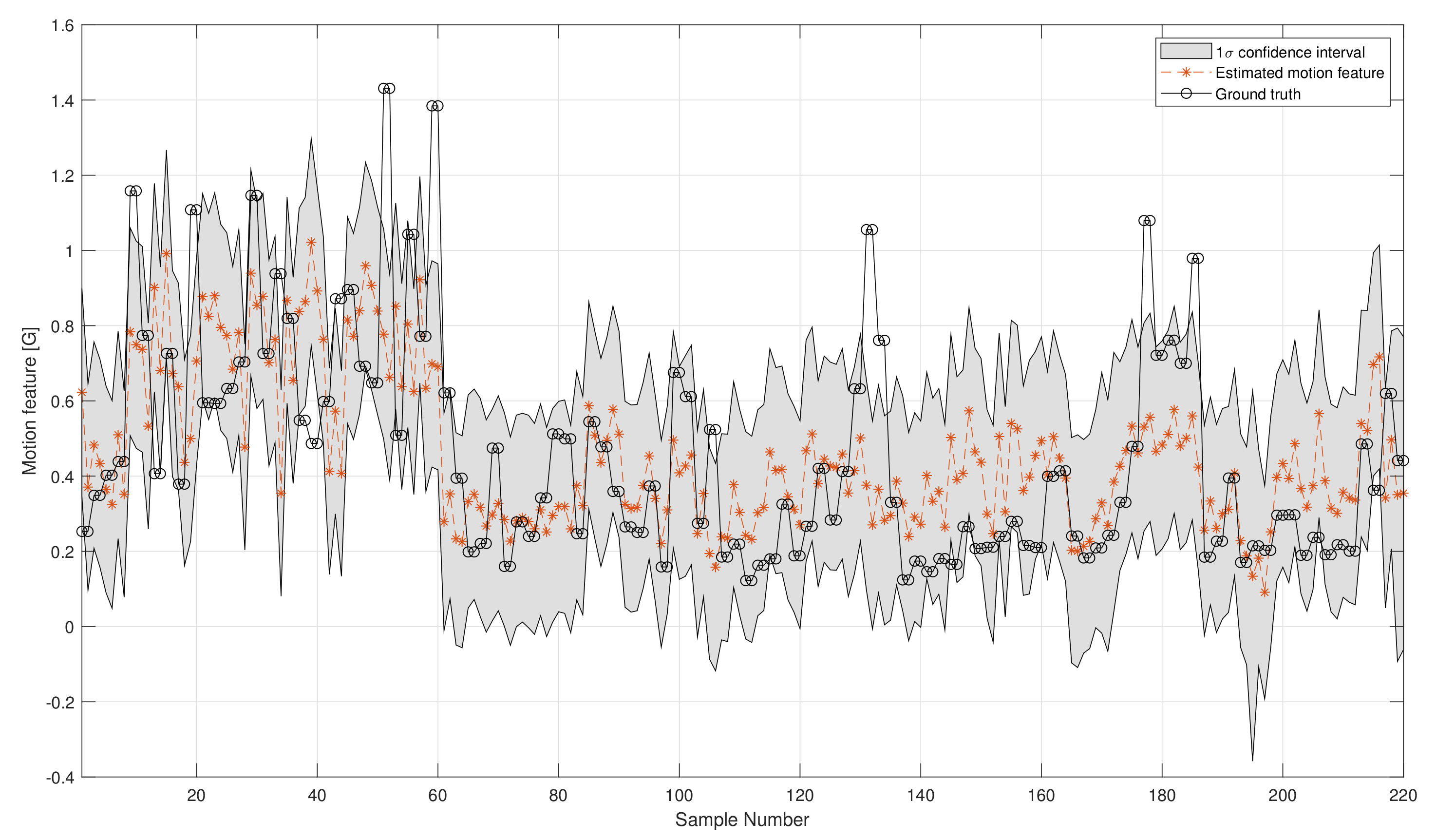
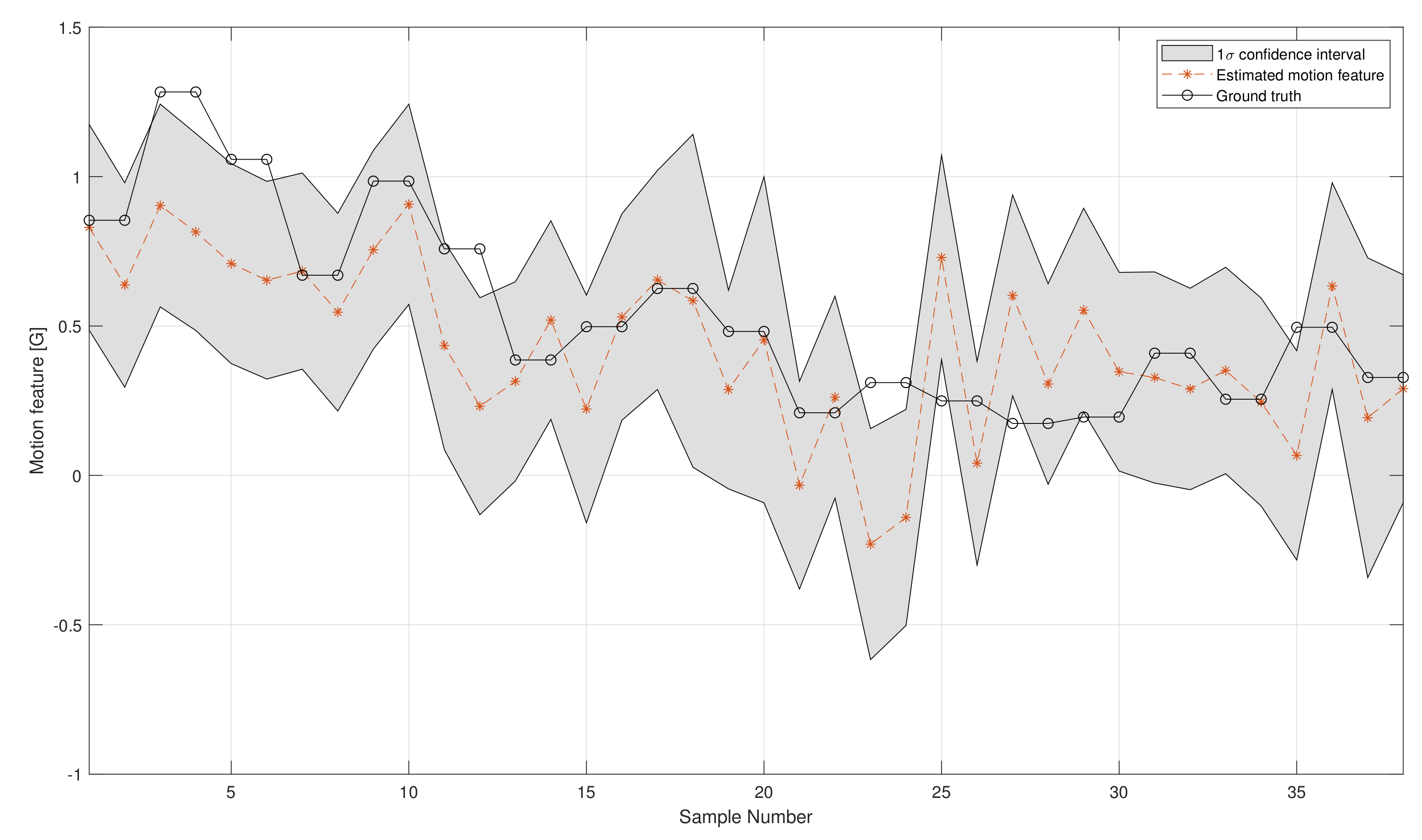
4.2. Results and Discussion

As a result of TNUD discrimination, training process for homogeneous and non-homogeneous terrains was achieved using 1956 and 368 observations, respectively. The predictions of the motion information for homogeneous and non-homogeneous terrains were generated using 220 and 38 image texture samples, respectively. To facilitate the interpretation of the regression results, we summarize the results in

Table 2. Prediction error.

Application of TNUD	Uniform terrains	0.2373
	Non-uniform terrains	0.268
Non-application of TNUD	-	0.3567

and plot the results of the predicted vibrations for both homogeneous and non-homogeneous terrains in Figure 13 and Figure 14. The error of the prediction for both homogeneous and non-homogeneous terrains is far lower than the prediction error of the regressor proposed in [24]. Moreover, the failed prediction error is also lower than the method proposed in [24]. The results are shown in

Table 3. Prediction error for failed cases.

Application of TNUD	Uniform terrains	0.4640
	Non-uniform terrains	0.4419
Non-application of TNUD	-	0.6048

.

The current framework sometimes fails to predict the vibrations in the terrain samples judged by the multiscale analysis to be either uniform or non-uniform. In the case of non-uniform terrains, as shown in Figure 14, the Gaussian process outputs negative predictions for vibration since we are not imposing any restrictions in this regard. Such negative vibration prediction is not consistent with the nature of the feature used in this study, which is always positive, as described by Equation (10). The only computations that are performed on the image are the global contrast measurement and contrast distance maps for scales 1, 2, and 3. The purpose of doing so was to understand and evaluate the behavior of the contrast distance feature toward non-uniformity. Multiscale analysis for scales 1, 2, and 3 suffers a slightly high computation time, as shown in

Table 4. Computation time.

Process	Computation Time
Multiscale analysis–contrast distance scale 1	880 ms
Multiscale analysis–contrast distance scale 2	200 ms
Multiscale analysis–contrast distance scale 3	47 ms
Multiscale analysis–fusion (refined contrast distance map)	2.2 ms
Texture extraction	67 ms
Motion feature	47 μs
Prediction for non-uniform terrains	100 ms
Predictor for uniform terrains	22 ms

. A scale 1 contrast distance map was generated with an image of size 1080 × 1920, a scale 2 contrast distance map was generated with an image of size 540 × 960, and a scale 3 contrast distance map was generated with an image of size 270 × 480. Since we could confirm that non-uniform regions have a higher contrast distance feature value than uniform regions, we propose in future work to accelerate this process by focusing only on the ROI and not the whole image. The ROI is approximately 10% of the whole image; thus, the computational time will decrease drastically.

Compared with [36], where motion prediction with varying speed based on the 3D reconstruction problem setting was investigated, our platform run at a constant speed of 0.2 m/s. We propose to study the effect of speed variations on the prediction of vibrations in future works.

5. Conclusions

In this paper, a traversability cost prediction was presented based on terrain non-uniformity detection for uneven outdoor terrain environments. The traversability cost was represented by the max-min difference of vertical acceleration of the mobile robot as a motion feature. Based on multiscale analysis of contrast distance feature maps, the non-uniformity of textures in an image is detected. Based on the discrimination of uniform/non-uniform terrains, the GP-based predictor is applied independently to learn the traversability cost. In the experiment, it was verified that the proposed non-uniformity detection helps to improve the prediction performance.

It was also observed in the experiment that it is naturally difficult to predict large accelerations on non-uniform terrains in certain cases. As future work, instead of applying the same framework of texture-based prediction to both uniform and non-uniform terrains, we can investigate a more suitable approach for the cost prediction of non-uniform terrains. In the case of complex mobile robot architectures, we expect that the same methodology can be applied by collecting motion data on various terrains and extending the framework to consider the mechanical properties as well as the correlation between speed of motion and traversability cost.

References

1. Sancho-Pradel, D.; Gao, Y. A survey on terrain assessment techniques for autonomous operation of planetary robots. J. Br. Interplanet. Soc. 2010, 63, 206–217. [Google Scholar]
2. Savkin, A.V.; Huang, H. Proactive Deployment of Aerial Drones for Coverage over Very Uneven Terrains: A Version of the 3D Art Gallery Problem. Sensors 2019, 19, 1438. [Google Scholar] [CrossRef] [PubMed] [Green Version]
3. Nagatani, K. Recent Trends and Issues of Volcanic Disaster Response with Mobile Robots. J. Robot. Mechatron. 2014, 26, 436–441. [Google Scholar] [CrossRef]
4. Zhou, F.; Arvidson, R.E.; Bennett, K.; Trease, B.; Lindemann, R.; Bellutta, P.; Iagnemma, K.; Senatore, C. Simulations of Mars Rover Traverses. J. Field. Robot. 2014, 31, 141–160. [Google Scholar] [CrossRef]
5. Mazhar, H.; Heyn, T.; Pazouki, A.; Melanz, D.; Seidl, A.; Bartholomew, A.; Tasora, A.; Negrut, D. CHRONO: A parallel multi-physics library for rigid-body, flexible-body, and fluid dynamics. Mech. Sci. 2013, 4, 49–64. [Google Scholar] [CrossRef] [Green Version]
6. Cunningham, C.; Ono, M.; Nesnas, I.; Yen, J.; Whittaker, W.L. Locally-adaptive slip prediction for planetary rovers using Gaussian processes. In Proceedings of the 2017 IEEE International Conference on Robotics and Automation (ICRA), Singapore, 29 May–3 June 2017; pp. 5487–5494. [Google Scholar]
7. Hong, T.; Chang, T.; Rasmussen, C.; Shneier, M. Road detection and tracking for autonomous mobile robots. In Proceedings of the SPIE Aeroscience Conference 2002, Orlando, FL, USA, 1–5 April 2002. [Google Scholar]
8. Manduchi, R.; Castano, A.; Talukder, A.; Matthies, L. Obstacle detection and terrain classification for autonomous off-road navigation. Auton. Robot. 2003, 18, 81–102. [Google Scholar] [CrossRef] [Green Version]
9. Suger, B.; Steder, B.; Burgard, W. Traversability analysis for mobile robots in outdoor environments: A semi-supervised learning approach based on 3D-lidar data. In Proceedings of the 2015 IEEE International Conference on Robotics and Automation (ICRA), Seattle, WA, USA, 26–30 May 2015; pp. 3941–3946. [Google Scholar]
10. Stavens, D.; Thrun, S. A self-supervised terrain roughness estimator for off-road autonomous driving. In Proceedings of the UAI’06, the Twenty-Second Conference on Uncertainty in Artificial Intelligence, Cambridge, MA, USA, 13–16 July 2006; pp. 469–476. [Google Scholar]
11. Ho, K. A Near-to-Far Non-Parametric Learning Approach for Estimating Traversability in Deformable Terrain. In Proceedings of the IEEE International Conference on Intelligent Robots and Systems, Tokyo, Japan, 3–7 November 2013; pp. 2827–2833. [Google Scholar]
12. Krebs, A.; Pradalier, C.; Siegwart, R. Adaptive rover behavior based on online empirical evaluation: Rover-terrain interaction and near-to-far learning. J. Field. Robot. 2010, 27, 158–180. [Google Scholar] [CrossRef]
13. Castelnovi, M.; Arkin, R.; Collins, T. Reactive speed control system based on terrain roughness detection. In Proceedings of the International Conference on Robotics and Automation, Barcelona, Spain, 18–22 April 2005; pp. 891–896. [Google Scholar]
14. Papadakis, P. Terrain traversability analysis methods for unmanned ground vehicles: A survey. Eng. Appl. Artif. Intel. 2013, 26, 1373–1385. [Google Scholar] [CrossRef] [Green Version]
15. Chilian, A.; Hirschmuller, H. Stereo camera based navigation of mobile robots on rough terrain. In Proceedings of the IEEE/RSJ International Conference on Intelligent Robots and Systems, St. Louis, MO, USA, 10–15 October 2009; pp. 4571–4576. [Google Scholar]
16. Hadsell, R.; Sermanet, P.; Ben, J.; Erkan, A.; Scoffier, M.; Kavukcuoglu, K.; Muller, U.; LeCun, Y. Learning long-range vision for autonomous off-road driving. J. Field Robot. 2009, 26, 120–144. [Google Scholar] [CrossRef] [Green Version]
17. Labayrade, R.; Gruyer, D.; Royere, C.; Perrollaz, M.; Aubert, D. Obstacle Detection Based on Fusion Between Stereovision and 2D Laser Scanner. Mob. Robot. Percept. Navig. 2007. [Google Scholar] [CrossRef]
18. Lalonde, J.-F.; Vandapel, N.; Huber, D.F.; Hebert, M. Natural terrain classification using three-dimensional ladar data for ground robot mobility. J. Field. Robot. 2006, 23, 839–861. [Google Scholar] [CrossRef]
19. Bellutta, P.; Manduchi, R.; Matthies, L.; Owens, K.; Rankin, A. Terrain perception for DEMO III. In Proceedings of the IEEE Intelligent Vehicles Symposium 2000 (Cat. No.00TH8511), Dearborn, MI, USA, 5 October 2000; pp. 326–331. [Google Scholar]
20. Brooks, C.A.; Iagnemma, K.D. Self-Supervised Classification for Planetary Rover Terrain Sensing. In Proceedings of the 2007 IEEE Aerospace Conference, Big Sky, MT, USA, 3–10 March 2007; pp. 1–9. [Google Scholar]
21. Brooks, C.; Iagnemma, K.; Dubowsky, S. Vibration-based Terrain Analysis for Mobile Robots. In Proceedings of the IEEE International Conference on Robotics and Automation, Barcelona, Spain, 18–22 April 2005; pp. 3415–3420. [Google Scholar]
22. Otsu, K.; Ono, M.; Fuchs, T.J.; Baldwin, I.; Kubota, T. Autonomous Terrain Classification With Co- and Self-Training Approach. IEEE Robot. Autom. Lett. 2016, 1, 814–819. [Google Scholar] [CrossRef]
23. Ho, K.; Peynot, T.; Sukkarieh, S. Nonparametric Traversability Estimation in Partially Occluded and Deformable Terrain. J. Field Robot. 2016, 33, 1131–1158. [Google Scholar] [CrossRef] [Green Version]
24. Bekhti, M.A.; Kobayashi, Y. Prediction of Vibrations as a Measure of Terrain Traversability in Outdoor Structured and Natural Environments. In Proceedings of the PSIVT 2015 Image and Video Technology, Auckland, New Zealand, 23–27 November 2015; pp. 282–294. [Google Scholar]
25. Rasmussen, C.E.; Williams, C.K.I. Gaussian Processes for Machine Learning (Adaptive Computation and Machine Learning); MIT Press: Cambridge, UK, 2006. [Google Scholar]
26. Howard, A.; Turmon, M.; Matthies, L.; Tang, B.; Angelova, A.; Mjolsness, E. Towards learned traversability for robot navigation: From underfoot to the far field. Field Robot. 2006, 23, 1005–1017. [Google Scholar] [CrossRef]
27. Chavez-Garcia, R.O.; Guzzi, J.; Gambardella, L.M.; Giusti, A. Learning Ground Traversability From Simulations. IEEE RA-L 2018, 3, 1695–1702. [Google Scholar] [CrossRef] [Green Version]
28. Metka, B.; Franzius, M.; Bauer-Wersing, U. Outdoor Self-Localization of a Mobile Robot Using Slow Feature Analysis. In Proceedings of the ICONIP 2013 International Conference on Neural Information Processing, Daegu, Korea, 3–7 November 2013; pp. 249–256. [Google Scholar]
29. Ordonez, C.; Collins, E.G. Rut Detection for Mobile Robots. In Proceedings of the SSST 2008 40th Southeastern Symposium on System Theory, New Orleans, LA, USA, 16–18 March 2008; pp. 334–337. [Google Scholar]
30. Collier, J.; Ramirez-Serrano, A. Environment Classification for Indoor/Outdoor Robotic Mapping. In Proceedings of the CRV 2009 Canadian Conference on Computer and Robot Vision, Kelowna, BC, Canada, 25–27 May 2009; pp. 276–283. [Google Scholar]
31. Chandler, D.M.; Vu, C.T. Main subject detection via adaptive feature refinement. J. Electron. Imaging 2011, 20, 013011. [Google Scholar]
32. Hartley, R.; Zisserman, A. Multiple View Geometry in Computer Vision, 2nd ed.; Cambridge University Press: Cambridge, UK, 2004. [Google Scholar]
33. Costa, A.F.; Humpire-Mamani, G.; Traina, A.J.M. An efficient algorithm for fractal analysis of textures. In Proceedings of the 25th SIBGRAPI Conference on Graphics, Patterns and Images, Ouro Preto, Brazil, 22–25 August 2012; pp. 39–46. [Google Scholar]
34. Liao, P.; Chen, T.; Chung, P. A fast algorithm for multilevel thresholding. J. Inf. Sci. Eng. 2001, 17, 713–727. [Google Scholar]
35. Bekhti, M.A.; Kobayashi, Y.; Matsumura, K. Terrain traversability analysis using multi-sensor data correlation by a mobile robot. In Proceedings of the 2014 IEEE/SICE International Symposium on System Integration, Tokyo, Japan, 13–15 December 2014; pp. 615–620. [Google Scholar]
36. Matsumura, K.; Bekhti, M.A.; Kobayashi, Y. Prediction of motion over traversable obstacles for autonomous mobile robot based on 3D reconstruction and running information. In Proceedings of the ICAM 2015 International Conference on Advanced Mechatronics, Tokyo, Japan, 5–8 December 2015. [Google Scholar]
Figure 1. Natural terrains. (a) Gravel; (b) Stones; (c) Non-uniform; (d) Grass; (e) Woodchip; (f) Non-uniform.
Applsci 10 01195 g001
Figure 2. Artificial terrains. (a) Slick asphalt; (b) Granulated asphalt; (c) Tiles; (d) Wood.
Applsci 10 01195 g002
Figure 3. Pioneer 3AT hardware configuration.
Applsci 10 01195 g003
Figure 4. Differential drive mobile robot.
Applsci 10 01195 g004
Figure 5. Overview of the proposed traversability cost prediction.
Applsci 10 01195 g005
Figure 6. Multiscale analysis for a homogeneous terrain.
Applsci 10 01195 g006
Figure 7. Multiscale analysis for a non homogeneous terrain.
Applsci 10 01195 g007
Figure 8. Refined contrast feature maps.
Applsci 10 01195 g008
Figure 9. Camera frame for mapping 3D point mapping onto the image plane.
Applsci 10 01195 g009
Figure 10. Mobile robot carrying a camera and layout of both world and camera reference frames.
Applsci 10 01195 g010
Figure 11. Identification of terrain patches for image feature extraction.
Applsci 10 01195 g011
Figure 12. Data acquisition.
Applsci 10 01195 g012
Figure 13. Prediction results for uniform terrains.
Applsci 10 01195 g013
Figure 14. Prediction results for non-uniform terrains.
Applsci 10 01195 g014