Abstract
As traditional automobiles develop towards new energy vehicles, the noise, vibration and harshness (NVH) performance of automobiles is facing new challenges. Without the cover of the traditional engine noise and inlet and exhaust noise, the high-speed wind noise becomes more prominent. Thus, research on the calculation method of vehicle interior noise in high-speed driving condition is needed. However, vehicle body structure is complex, and the external excitation components are complicated. In order to analyze the method of predicting the vehicle interior noise at high speed, an idealized side mirror model is taken as the research object in this paper and the radiated noise of a panel under the fluctuating surface pressure (FSP) due to the idealized side mirror is studied. The FSP of the panel is first studied by the numerical simulations of incompressible and compressible flow field. For the incompressible flow field, the Corcos turbulent boundary layer (TBL) model is established to simulate the convective component and the boundary element method (BEM) is used to extract the acoustic component. Subsequently, the Corcos model coupling BEM method, the random modal force coupling BEM method and the deterministic modal force coupling BEM method are used separately to calculate the noise of the panel under the FSP. For the compressible flow field, the convective and acoustic component in the fluctuating pressure are separated by the wavenumber-frequency spectrum (WFS) method. The radiated noise of the panel under the FSP is calculated again by using the WFS, the method of random modal force and the method of deterministic modal force, respectively. Then, the computational time of the six methods of incompressible and compressible calculation is compared. Finally, a fast and accurate method of calculating the panel radiated noise under FSP is obtained by comparing the computational accuracy with the experimental results and combining the computational time: the method of incompressible random modal force. This method can be used to quickly and accurately analyze the vehicle interior noise at high speed, and to optimize the exterior protrusions and the vehicle sound package for improving the vehicle NVH performance at high speed.
1. Introduction
The wind noise sources generated by turbulent flow play an important role to the interior noise sound pressure level (SPL) of the vehicle. Bremner et al. [1] first used the wavenumber-frequency spectrum (WFS) to analyze the excitation component of the external flow field. It was found that the acoustic component with the low wavenumber in the external flow field has a great influence on the sound transmission of the structure exposed in the flow field, but the low wavenumber component of turbulent boundary layer (TBL) cannot be defined. The wind tunnel test, the transient computational fluid dynamics (CFD) simulation and the WFS analysis are used to verify the existence of the acoustic component of the outflow field in [2,3,4]. In order to analyze the effect of the acoustic component on the interior noise SPL of the vehicle, the characteristics of the acoustic component were studied. The researches show: both the convective and acoustic component are equally important contributors for the noise transmission to the vehicle cabin although the TBL pressure is 25 to 35 dB higher in level than that of the corresponding acoustic component [1].
There are many kinds methods for calculating the response under the TBL excitation. One of the models for the TBL is presented by Corcos [5]. Then, Chase and Efimstov built models derived from Corcos expression, which can improve the predictions for the low-frequency range [4,6]. Birgersson et al. [7] used the Chase-like model and Corcos model to describe the wall pressure excitation of the TBL flow, and compared and analyzed the results of TBL calculated by the two models. Ichchou et al. [8] developed a “rain on the roof” excitation equivalent to acoustic and aerodynamic excitation. The model was equivalent in wavenumber space. The TBL excitation was verified based on the Corcos model, which proved the effectiveness of predicting the power spectral density (PSD) of the velocity. Chronopoulos D. et al. [9] used a second order moment matching method based on previous studies to achieve a fully coupled structural progression system that reduced the wide-band frequency range under actual aerodynamic distributed excitation. It also described the expression form of TBL equivalent correlation function when it was applied on a plate. Ciappi et al. [10] studied the response of composite plates under the TBL excitation and performed numerical and experimental studies. Marchetto et al. [11] developed a method to characterize the vibration response method of the plate to the diffuse acoustic field (DAF) excitation based on the DAF theoretical model and the sensitivity function of the plate.
Because the acoustic component can be easily coupled with the radiating modes of the panel [12], Smith et al. [13] designed an experiment to analyze the sound radiation of a car window under the flow-induced excitation, but no acoustic component was found due to the aliasing effect. Later, Bremner [14] and Mendonca et al. [15] demonstrated the existence of the acoustic source through the CFD compressible flow simulation with the wavenumber-frequency method. In order to capture the acoustic component, the CFD compressible turbulent flow data is necessary if the acoustic wind tunnel (AWT) is not available. Besides, there are many practical difficulties to separate out the acoustic component in the AWT test, such as the transducer size and locations, the background noise, etc. Moreover, the CFD compressible method is time-consuming and the grid size needs to be very small to capture the acoustic component. However, the CFD incompressible flow simulation costs less time and can be conducted easily. So, how to predict vehicle interior noise accurately based on the CFD incompressible flow data is a concern. Blanchet et al. [16] proposed several models to predict cabin interior noise based on the CFD compressible, incompressible simulation and experiment results, but no comparison between different models was acquired. Therefore, this paper focuses on finding out a proper method to predict the radiated noise of a panel under the fluctuating surface pressure (FSP) due to an idealized side mirror. The FSP of the idealized side mirror is firstly analyzed by the incompressible and compressible numerical simulations. Then, based on the FSP of the incompressible and compressible numerical simulations, the aerodynamic noise analysis of the panel is respectively performed by the six methods. By validating with the experimental data and comparing the computing time of all six methods, the method of random modal force coupling boundary element method (BEM) under the incompressible numerical simulation is proposed to predict the radiated noise of the panel under the aerodynamic load. This method can be used to predict the vehicle interior noise at high speed. At different stages of automobile development, an appropriate method can be selected for different purposes in terms of the accuracy of results and computing time.
2. Fluctuating Pressure Analysis of Idealized Side Mirror
2.1. 3D Model
An idealized side mirror model is used as the research object. It consists of a half cylinder and a quarter of a sphere. The diameter of the cylinder is and the height is , as shown in Figure 1a. In order to prevent the computational domain boundary from interfering with the flow field, it is required that the computational domain fully includes the eddy current region generated by the side mirror when lengthwise. Meanwhile, in order to minimize the inhomogeneity of the stagnation parameters, the inlet should be kept at a distance from the side mirror. The length, width and height of the computational domain are , and , and the distance between the inlet of the side mirror and computational domain is , as shown in Figure 1b.
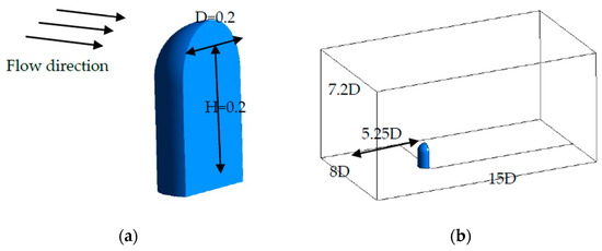
Figure 1.
(a) The model of an idealized side mirror. (b) The dimension of the computational domain and the distance between the inlet of the side mirror and computational domain.
A panel is separated behind the side mirror to simulate vehicle side window. The TBL generated on the panel is used to simulate the flow state of the air flow on the side window. A small panel behind the side mirror is used to simulate the size of the side window. The material of the panel is aluminum, and the specific parameters are shown in Table 1.

Table 1.
Panel parameter.
The panel is divided into finite element meshes and the mesh size is . Figure 2a shows the position relationship between the panel and the side mirror. The distance between the receiver point and the panel is , as shown in Figure 2b.
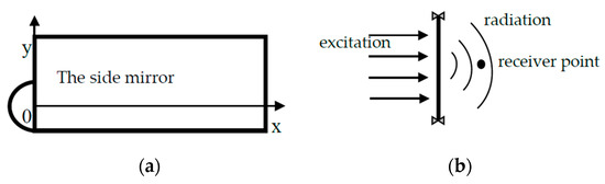
Figure 2.
(a) The position relationship between the panel and the side mirror (b) The distance between the receiver point and the panel.
2.2. Incompressible Numerical Simulation
The whole computational domain is divided into several regular regions by the block method in the integrated computer engineering and manufacturing (ICEM). The hexahedral mesh is used, and the boundary layer mesh is created on the surface of the side mirror. The final number of grid elements is about 7 million and the quality of the mesh is very good. Near-wall layer extrusions is built to resolve the boundary and adverse-pressure-gradient flow separation with fine mesh. The minimum mesh size is and meets the requirement of at least six elements per wavelength. Figure 3 shows the results of meshing in the computational domain.
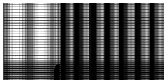
Figure 3.
Result of meshing in computational domain.
The fluctuating pressure distribution of airflow through the side mirror is calculated by using the software FLUENT. The airflow velocity is , and the inlet condition is velocity-inlet. Meanwhile, the turbulence length scale L and turbulence intensity I are set as and . and are the turbulent fluctuating velocity and the average velocity. is the Reynolds number calculated by characteristic dimension D(). is the air density at . is the current speed. is the aerodynamic viscosity at . For the set of the boundary conditions of the model, the outlet condition is pressure outlet at because the reference pressure is 1 atmospheric pressure. The turbulence length scale L and turbulence intensity I at the outlet are set to be the same as that at the inlet. The setting of boundary conditions is shown in Table 2.
Table 2.
Settings of boundary conditions.
The highest frequency of the calculation is , time step size , and the total time is .
The pressure distribution nephogram of the bottom panel of the side mirror is shown in Figure 4. We can see that the local pressure in front of the side mirror is high and forms a horseshoe vortex. The pressure on the left and right side and the back of the side mirror is relatively low. The pressure distribution on the back of the side mirror is uneven and there is vortex.
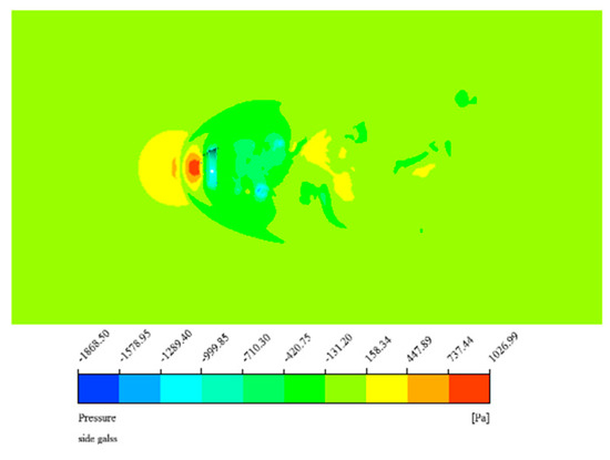
Figure 4.
Distribution of pressure at the bottom panel of the side mirror.
Figure 5 shows the velocity vector and local enlarged drawing of section. We can see that the presence of the side mirror results in a lower airflow velocity on the back of the mirror, and the air velocity around is higher. Because of the airflow velocity difference, the high-speed airflow flows continuously to the region of low-speed airflow and forms counter-current and vortices. The maximum velocity occurs on the top of the side mirror surface, about , which is 30%~50% higher than the velocity of the flow field. After the top, the airflow gradually separates from the side mirror. Instead of following the radian of the side mirror, it extends backward along the horizontal direction and results in a separation zone. The length of the separation zone is about two times the length of the side mirror. Then the airflow contacts the ground again and results in the re-attachment zone. Figure 5b clearly shows the velocity changes around the side mirror. The periodic vortex shedding phenomenon at the junction of the side mirror and the ground causes the fluctuating pressure of the surrounding air to change continuously with time.
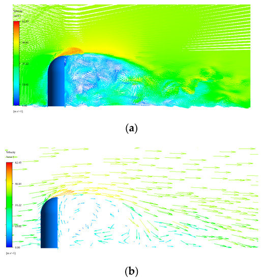
Figure 5.
(a) Velocity vector map of the side mirror. (b) Local magnification of the side mirror velocity vector map.
2.3. Compressible Numerical Simulation
In order to study the numerical calculation of the flow field of compressible fluid flowing around the side mirror, the size of the side mirror and the calculation domain are kept unchanged. Meanwhile, in order to capture the acoustic component, the mesh is partially refined. The block method is used in ICEM to divide the structural meshes into hexahedral meshes. The total number of meshes is about 19.28 million, and the minimum mesh size is . The boundary layer mesh is generated around the mirror surface to capture vortex characteristics. The side view of the entire computational domain grid is shown in Figure 6.
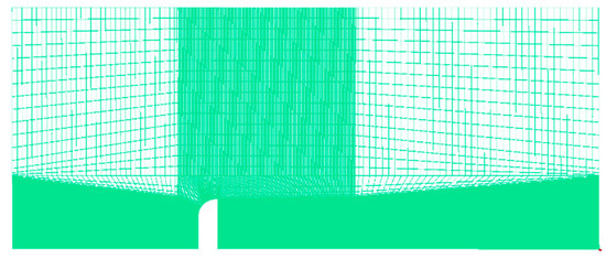
Figure 6.
Compressible computing mesh generation.
In the material setting, the gas is set to ideal-gas, and the compressibility of the gas is considered. Viscosity is set to the Sutherland formula with three coefficients. The setting of boundary conditions is also different from that of the incompressible computation. The inlet boundary condition is set to the far-field pressure inlet. Because the Mach number is 0.118 when the velocity is , the inlet boundary condition is set to 0.118 and the relative pressure is set to . The far field of pressure is also set on the left and right sides and on the top, so that the acoustic will not produce reflex, scattering and other erroneous acoustic results [17].
In calculation, two-equation turbulence model is used to calculate the quasi-steady solution of the flow field in 1000 steps, and then the large eddy simulation is used to calculate the unsteady flow field of the side mirror; for the sub-lattice model, the Smagorinsky-Lilly model [18] is used. The initial time step is set to , in a single time step there are 25 iterations. After 2000 steps’ calculating, the initial step is kept unchanged, and the time step is set to 5000 steps.
The pressure distribution of the panel is shown in Figure 7. For the back areas of the side mirror, the area of the length of the side mirror represents negative pressure and the other following areas show positive pressure. Horseshoe vortices are generated on the panel in front of the side mirror, where the positive pressure reaches the maximum.
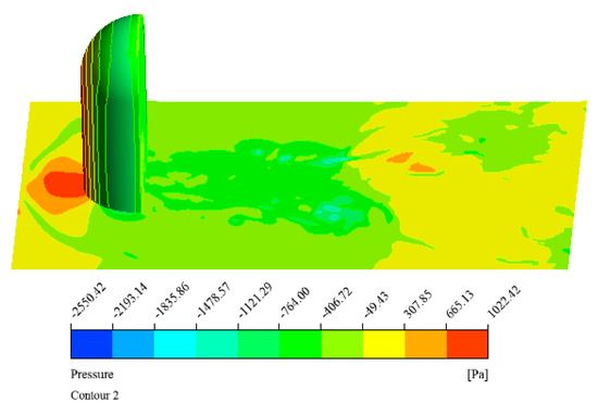
Figure 7.
Pressure distribution of the side mirror and the panel.
Figure 8 shows the velocity vector of the plane. Compared to the incompressible computation, the compressible computation captures smaller eddies and makes finer velocity vectors. The eddy current behind the side mirror can be clearly observed. The velocity behind the side mirror is the lowest, and the velocity at the top of the side mirror is the highest. Then the velocity gradually returns to the normal value.
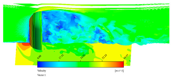
Figure 8.
Velocity vector diagram for plane.
The fluctuating pressure is generated on the side mirror and the panel and includes monopoles, dipoles and quadrupole sources simultaneously on the side mirror and the panel. Single and quadrupole sources are not considered here. The Curle dipole source is shown in Figure 9. The dipole source on the surface of the side mirror is the largest, and the sound source along both sides of the side mirror is also very large. The sound source on the panel presents a random distribution.
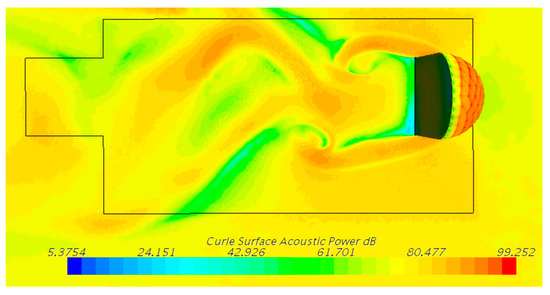
Figure 9.
Distribution of sound sources on the side mirror and Curle surface of the panel.
3. Aerodynamic Noise Analysis of the Panel
3.1. Incompressible Numerical Simulation
3.1.1. Convective Component of FSP
(a) Corcos Model
There are several empirical wavenumber-frequency surface pressure models that can be used to extract the convective component. The most commonly used and widely accepted model is the Corcos model [5]. The model supposes that the waves travelling streamwise are independent of the waves travelling across to the stream. So streamwise decay and cross stream decay can be gained separately. Another assumption is that the spatial correlation of fluctuating surface pressure is homogenous within a given flow zone and the WFS over that zone is approximately equal to the product of space-averaged pressure spectral density and the spatial correlation. The Corcos model can be expressed as follows
where, and represent the decay of surface pressure coherence in streamwise and cross flow direction. is the space-averaged pressure PSD. They are chosen to yield the best agreement with the experiment data. After the two-dimensional wavenumber transform of Equation (1), one finds [19]:
Firstly, the area calculated is divided into several small areas. For each area, the cross-spectrum between any two nodes in the direction of airflow and the direction of vertical airflow is obtained, and the cross-spectrum matrix is formed. Because the number of nodes is very large, the cross-spectral matrix of each small area is averaged to reduce the computational complexity. Then the cross-spectra of these small regions are averaged to obtain the spatial correlation function .
After obtaining the phase of the spatial correlation function, the wavenumber along the direction of the airflow is obtained using the following Equation (3). The attenuation coefficients along the airflow direction and across airflow direction are obtained by using the following Equations (4) and (5).
Four parameters of the Corcos model (convective velocity , attenuation coefficient along the airflow direction, attenuation coefficient in the vertical airflow direction, and spatial average pressure spectrum ) are obtained. Figure 10 shows the spatial average pressure obtained by means of the Corcos model. The wavenumber in the X direction is , . U is the airflow velocity. The dissipation coefficients in X and Y directions are 0.1 and 0.72.
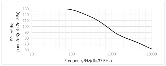
Figure 10.
Spatial average pressure obtained by means of the Corcos model.
In Figure 10, we can see that the SPL on the surface of the panel decreases rapidly from 0 to 1000 Hz, and gently above 1000 Hz. Most of the energy of the convective component is concentrated in the middle and low frequencies. When the Corcos model is used to extract the convective component, the panel is required to build a statistical energy analysis (SEA) model. LeVitte [20] proposed to calculate the local input power of the SEA model by using Equation (6)—concerning the properties and fluid parameters of the SEA structural subsystem.
is the input power of the calculation area. is the modal density. is the surface density. is the modal joint acceptance.
(b) Methods of Random Modal Force and Deterministic Modal Force
When the finite element analysis (FEA) panel is used as the research object, the time-domain fluctuating pressure of the CFD simulation results can be projected to the nodes of the panel. According to whether the grids of the panel coincide with the acoustic grids in CFD calculation, the corresponding projection mode can be deterministic. If it is consistent, it can be directly loaded to the nodes of the panel. If the acoustic grids are larger than the grids of the panel, the average value of the fluctuating pressure at the nodes of CFD grid is usually taken and then loaded to the nodes of acoustic grids. The fluctuating pressure excitation can be finally loaded to the FEA panel. Before loading the excitation, it is necessary to calculate the modes of the panel. Thus, the method of loading the excitation is called the method of modal force.
For the deterministic modal force, it is obtained in frequency-domain by using the Fourier transform of the whole time signal without pre-processing the data. Then, the deterministic modal force is projected to the nodes of the FEA panel. For the random modal force, the time domain modal force signal is divided into L segments and each segment of data allows the overlap. The self-PSD of each segment is calculated by using Fourier transform and is performed to smooth the spectrum with the appropriate window function. Then by averaging the data, the random modal force is obtained. The more segments the time-domain signal is divided into, the smaller the variance will be. The variance characteristics of the data can be improved, but the overlap of data will reduce the irrelevance between each segment of data and make the reduction in variance lower than the theoretical value. In this paper, the data is divided into eight segments, and the overlap rate between each segment is 50%.
3.1.2. Acoustic Component of FSP
Because the acoustic component cannot be extracted from the FSP obtained by the incompressible numerical simulation of the flow field outside the side mirror, Lighthill Curle acoustic analogy method combined with BEM is used to obtain the SPL radiated by the fluctuating pressure on the surface of the side mirror as the acoustic component of the FSP. Because the fast multipole boundary element method (FM-BEM) can save much more computing time and reduce the more memory requirements greatly than the conventional boundary element method (CBEM), the FM-BEM method is used to solve the acoustic component. The FM-BEM model of the side mirror and the panel is established in VA One [21], as shown in Figure 11. All surfaces of the side mirror are rigid boundaries and the panel is used as the data recovery surface. The FSP of time series is used as the excitation source. By using Lighthill Curle acoustic analogy method, the root mean square (RMS) value of the space average pressure on the surface of the side mirror is obtained as shown in Figure 12. At middle-low frequency, the FSP of the side mirror decreases quickly. Most of the energy of the FSP of the side mirror lies at lower frequency.
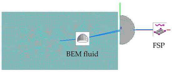
Figure 11.
The FM-BEM model of the side mirror and the panel.
Figure 12.
The RMS of the space average pressure on the side mirror surface.
Figure 13 shows the pressure RMS distributions of the panel for 315 Hz, 1000 Hz, 3150 Hz and the overall pressure under the FSP of the side mirror. We can see that the main energy of the acoustic component is concentrated near the side mirror, and the pressure RMS of the acoustic component increases gradually with the increase in frequency.
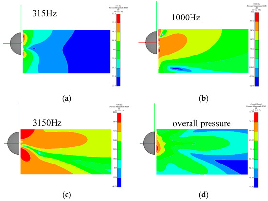
Figure 13.
The pressure RMS distributions of the panel for 315 Hz, 1000 Hz, 3150 Hz and the overall pressure under the FSP of the side mirror: (a) For 315 Hz; (b) For 1000 Hz; (c) For 3150 Hz; (d) For the overall pressure.
3.1.3. Aerodynamic Noise Analysis
(a) Mechanism of Radiated Sound under Aerodynamic Load
Compared with the aircraft TBL, the flow speed past a car is relatively small and—particularly—the vortex happens when it meets irregularly shaped bodies. The flow past a car is an aero-vibro-acoustic problem. Strumolo [22] had proposed the sound power radiated from the panel vibration as follows:
where, is air density. is air speed. is area of the panel. is radiation efficiency. is velocity spectral density.
The radiation efficiency in terms of the wavenumber and the velocity spectral density is given by [23]:
where, , is the shape function. is the excitation source. is the structural modal impedance. is the modal mass and is the modal admittance. is the WFS.
Later, Bremmer [14] separated the formula of the sound power into resonant and non-resonant contributions without considering stiffness-controlled modes. Then Equation (7) can be written as:
where, the modal joint acceptance is as follows:
where, is the surface area of the panel.
The (m, n)th simply supported mode shape is as follows:
where, and are the length and width of the panel, respectively. The amplitude of the shape function is given by:
The amplitude of the shape function reaches peak around the modal wavenumbers and . There are an infinite number of side lobes at each side of the peak, as shown in Figure 14. We can see that has peaks around the modal wavenumber . Meanwhile, the WFS of the boundary layer pressure achieves the maximum value when , ( is convective velocity). Therefore, the highest excitation occurs when the modal wavenumber () close to , , namely the hydrodynamic coincidence condition.
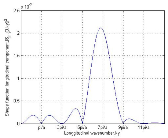
Figure 14.
Squared magnitude of the shape function with , .
The side window is usually approximated as a thin panel with thickness and density . The lateral displacement of the panel under a pressure loading described by Kirchhoff plate theory [24] is written as follows:
where, is the Laplacian operator. is the bending stiffness of the panel and is the product of Young’s Modulus and the moment of inertia .
where, is the Poisson’s ratio.
The acoustic wavenumber, convective wavenumber and panel wavenumber are three important wavenumbers to analyze the hydrodynamic coincidence and acoustic coincidence effect. The panel wavenumber is calculated as follows:
The acoustic wavenumber is simply the frequency divided by the speed of sound. The convective wavenumber is the frequency divided by the convective speed:
According to the physical parameters and Equation (15), the wavenumber curve of the panel with frequency can be calculated, and the wavenumber of the convective and acoustic components can also be calculated according to Equation (16). The results are shown in Figure 15. In this figure, we can see that there is an intersection point between the wavenumber of the panel and the wavenumber of the convective component and the wavenumber of the acoustic component at 400 Hz and 3150 Hz, corresponding to the aerodynamic coincidence effect and the vibro-acoustic coincidence effect. Under these two frequency points, the excitation of the convective component and the acoustic component reaches the maximum.
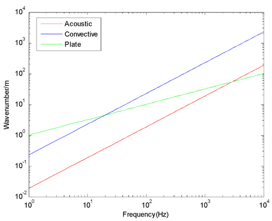
Figure 15.
The wavenumbers. (Red curve, blue curve and green curve represent the wavenumbers of the acoustic component, the convective component and the panel, respectively).
(b) Aerodynamic Noise Analysis Model
For the incompressible numerical simulation of the FSP, the convective component is obtained by the Corcos model, random modal force and deterministic modal force, and the acoustic component is obtained by the BEM method. Therefore, for the incompressible numerical simulation of the FSP, the Corcos model coupling BEM method, random modal force coupling BEM method and the deterministic modal force coupling BEM method are used to solve the aerodynamic noise of the panel. Firstly, the Corcos model in TBL is used to calculate the convective component and DAF is used to represent the acoustic component. The model of Corcos model and DAF is shown in Figure 16. The panel is a SEA panel, and a semi-infinite fluid (SIF) is used to obtain the SPL at the SIF location.
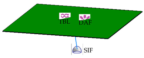
Figure 16.
The model of Corcos model and DAF.
For the convection component characterized by the random modal force or deterministic modal force, the loading object is required to be a FEA structure. Therefore, the panel should be meshed. The boundary conditions by simulating the real side window and the material properties of the panel should be set up, and then the modal of the panel should be solved. The modal results of the panel solved in Nastran are shown in Figure 17. The first natural frequency is 153.2 Hz and the second natural frequency is 398.49 Hz. The vibro-acoustic model established by the method of random modal force and deterministic modal force is shown in Figure 18. The two FSPs represent the convective component and the acoustic component. SIF is used to capture the SPL at the receiving point.
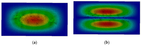
Figure 17.
Modes of the panel: (a) 153.2 Hz; (b) 398.49 Hz.
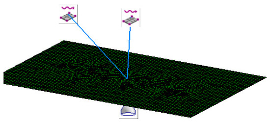
Figure 18.
Vibro-acoustic model of the random modal force and deterministic modal force.
(c) Result Analysis
The SPLs radiated from the position of 0.1 m away from the panel under the excitation of the Corcos model with and without the acoustic component are shown in Figure 19. In this figure, we can see that the radiated SPL of the panel with the excitation of the acoustic component is 2~5 dB higher than that of the panel without the excitation of the acoustic component at 2500 Hz. Thus, the excitation of the acoustic component has a great influence on the radiated SPL in high frequency band. In order to accurately predict the radiated noise of the panel under the FSP, the effect of the acoustic component cannot be neglected. Meanwhile, the radiated SPL has a peak at 3150 Hz, which shows the coincidence effect when the wavenumber of the panel is equal to the wavenumber of the acoustic component.
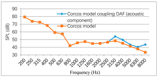
Figure 19.
Radiated SPLs of the panel under the Corcos model coupling DAF and only the Corcos model.
The results of the radiated SPLs of the panel calculated by the random modal force coupling BEM and the deterministic modal force coupling BEM are shown in Figure 20 and Figure 21. Likewise, we can see that the radiated SPL of the panel coupling the excitation of the acoustic component is higher than that of the panel without the excitation of the acoustic component. It is consistent with the calculation results of the Cocos Model coupling BEM model. In Figure 20, the peak value of the random modal force coupling the acoustic component occurs at 4000 Hz, and the radiated SPL is not only related to the magnitude of excitation, but also to the resonance of the panel. One of the resonance frequencies of the panel is 4006.7 Hz, so there is a large peak value of the radiated SPL by the panel at this frequency. Another peak at 400 Hz is due to the aerodynamic coincidence effect.
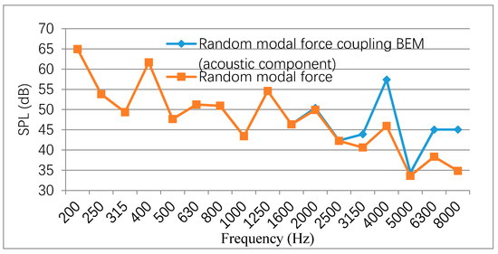
Figure 20.
Radiated SPLs of the panel under the random modal force with and without the acoustic component.
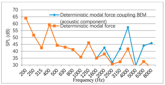
Figure 21.
Radiated SPLs of the panel under the deterministic modal force with and without acoustic component.
In Figure 21, it is possible to appreciate that the difference between the results of the deterministic modal force with and without the excitation of the acoustic component is greater than that of the random modal force method. That is because the signal averaging and smoothing are performed by using the method of random modal force to make the signal more stable than the method of deterministic modal force.
3.2. Compressible Numerical Simulation
3.2.1. WFS Analysis
(a) Layout of Receiver Points and Cross-PSD
A total of 1384 receiver points are arranged on the panel, as shown in Figure 22. The distance between each receiver point along the direction of airflow, i.e., x direction, is 0.001 m, and the distance between each receiver point in the longitudinal direction is 0.002 m. In Figure 22, P1 represents 571 receiver points along the airflow direction at the symmetrical line of the side mirror. P2 represents 571 receiver points at 1/2 of the side mirror diameter along the X axis. A total of 121 receiver points are arranged at T1 and T2 locations, which are 0.4 m and 0.6 m away from the coordinate origin. The cut-off frequency is related to the distance between monitoring points, which can be expressed by Equation (17). Since the minimum distance between the two receiver points is 0.001 m, by assuming the convective velocity , the cut-off frequency is 8800 Hz.
where, is the distance between the two receiver points along the direction of flow.
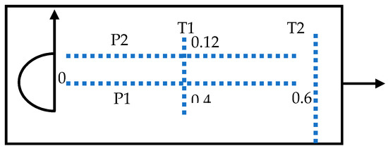
Figure 22.
The arrangement of the receiver points on the panel.
After obtaining the FSP of 1384 receiver points, the pressure of time series receiver points need to be transformed into the pressure in frequency-domain by the Fourier transform. is a random static ergodic signal in time and space domain. Its Fourier transform is as follows:
where, T is the time interval.
The cross-PSD is defined as:
where, is a mathematical expectation.
In uniform field, the cross-PSD is only a function of distance , i.e., . Its spatial Fourier transform is the expression of the cross-PSD in frequency-domain and wavenumber domain, which is usually called the WFS.
It can be seen that the key to solving the WFS is to solve the cross-PSD.
In this paper, the Welch method is used to estimate the average power spectrum:
where is a finite sequence of points, M is a sample point, L is a segment number, , , is a normalization factor, is a data window.
(b) WFS Analysis
The WFS analysis is used to calculate the FSP distribution of the panel in time and space domain. According to the SPL and space-time Fourier transform of the receiver points calculated by the compressible numerical method, the WFS of the panel can be calculated by Equation (21), as shown in Figure 23. The wavenumber in the positive direction of is along the airflow direction, and the velocity in the negative direction represents the opposite direction of the airflow. Similarly, the wavenumber in the positive direction of represents the positive direction of Y in the vertical flow direction, and the wavenumber in the negative direction of represents the negative direction of .
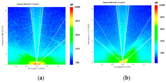
Figure 23.
WFS in the X and Y directions of the panel: (a) ; (b) .
In Figure 23, there are wavenumbers along the airflow direction and in the vertical airflow direction. The place where the energy is concentrated and the color is deepest represents the convective component, which is represented by using the white line to fit the direction of convective velocity. The slope of the fitted white line can calculate the convective velocity . The convective component shows directionality in the X direction and no directionality in the Y direction. In addition, no matter in the X direction or the Y direction, there is an obvious energy concentration around the positive and negative and , which is the acoustic component.
Figure 24 shows the wavenumber diagrams of the panel. In Figure 24, at , the convective component plays the major role, and the presence of the acoustic component cannot be observed in the white circle. With the increase in frequency, the color in the white circle deepens gradually. That means that the energy of the acoustic component increases gradually. At , it can be clearly seen that the energy of the acoustic component is very large. Therefore, the acoustic component can not be neglected when calculating the radiated noise of the panel under FSP, especially at high frequencies.
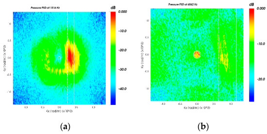
Figure 24.
Wavenumber diagrams at different frequencies: (a) 1516 Hz; (b) 4042 Hz.
3.2.2. Aerodynamic Noise Analysis
For the compressible numerical simulation of the FSP, the results of the WFS analysis show that the compressible numerical simulation of the FSP includes not only the convective component, but also the acoustic component. Therefore, for the compressible numerical simulation, the aerodynamic noise of the panel can be analyzed by using the convective and acoustic component obtained by the WFS analysis, random modal force and deterministic modal force.
The convective and acoustic component obtained by the WFS analysis are represented by the TBL and DAF model. The TBL coupling DAF model of the WFS analysis is consistent with the model of Corcos model coupling BEM method of the incompressible numerical simulation. Figure 25 shows the results of the radiated SPL of the compressible numerical simulation comparing that of the incompressible numerical simulation. We can see that there is a peak value of the radiated SPL of the panel in the compressible numerical calculation at , which is consistent with the results of the incompressible numerical simulation. However, the results of the compressible numerical simulation are smaller at high frequencies. That is because the acoustic component calculated by the BEM method is indirectly calculated by using the dipole source on the surface of the side mirror as the excitation, while in the compressible numerical simulation, the convective component and the acoustic component are calculated simultaneously. The size of the mesh and the size of the calculation domain will affect the extraction of the acoustic component and possibly conceal the acoustic component. However, from the compressible calculation results, it can be seen that the method can generally predict the trend of radiated SPL under the FSP, and can accurately reflect the influence of the acoustic component.
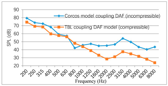
Figure 25.
Comparison of the results of Corcos model coupling DAF under the incompressible numerical simulation and TBL coupling DAF model of WFS under the compressible numerical simulation.
The FEA panel of the compressible model for deterministic modal force or random modal force is consistent with the incompressible numerical simulation model, as shown in Figure 26. Because the FSP obtained by the compressible numerical simulation includes the acoustic component, there is no need to extract the additional acoustic component. Only the FSP excitation is applied to the FEA panel. A SIF is used to calculate the radiated SPL at the receiving point.
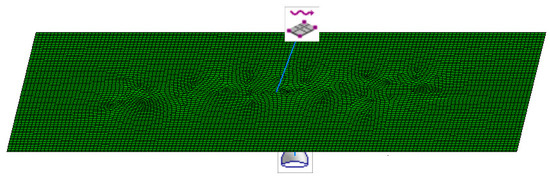
Figure 26.
Compressible model of the random modal force and deterministic modal force.
The data is also divided into eight segments using the calculation of the random modal force, and kept the overlap rate of each segment unchanged by 50%. For the method of deterministic modal force, the FSP is projected directly to the nodes of the panel, and the results are shown in Figure 27. In this figure, it can be seen that the calculated results of the compressible modal force are consistent with those of the incompressible random modal force, namely that the radiated SPL of the panel under the random modal force is larger than that under the deterministic modal force.
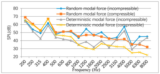
Figure 27.
Comparison of the results of the random modal force and deterministic modal force under the incompressible and compressible numerical simulations.
4. Validation and Comparison of Analytical Methods
4.1. Validation of Simulation Analysis
In order to compare the differences between the six methods more clearly, and to compare the accuracy of the calculation results of each method, the results are compared with the experimental results obtained by Bremner [14] in the Wind Tunnel Laboratory of Southampton University. The experimental setup was defined by the idealized side mirror model and the panel shown in Figure 1. The layout of surface pressure microphone arrays on the panel behind the idealized side mirror are shown in Figure 22. Therefore, the experimental data can be used to estimate the numerical results.
Figure 28 shows the comparison between the results of the three methods under the incompressible numerical simulation and the experimental data. In Figure 28, it can be seen that under the incompressible numerical simulation, the result of the method of random modal force coupling BEM method is closer to the experimental data than that of other methods.
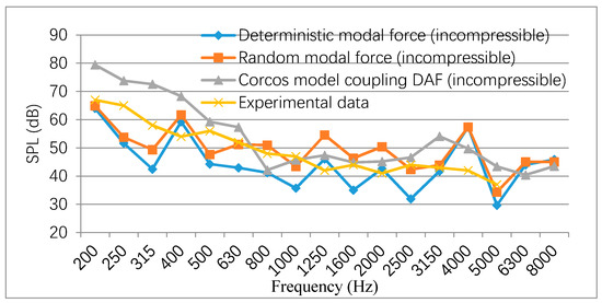
Figure 28.
Comparisons of the results of BEM coupling three methods of incompressible numerical simulation and experimental result.
Figure 29 shows the comparison between the results of the other three methods under the compressible numerical simulation and the experimental data. In Figure 29, the result of the method of random modal force by the WFS method is closer to the experimental data than that of other methods in the compressible numerical simulation. The difference between the experimental data and the result of the method of random modal force by the WFS method is approximately less than 3 dB. Therefore, the method of random modal force obtained by the WFS method is proposed to calculate the radiated SPL of the panel under the FSP without considering the calculation time.
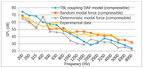
Figure 29.
Comparisons of the results of the WFS coupling three methods of the compressible numerical simulation and experimental result.
4.2. Comparison of Calculation Time
In order to compare the computational time of each method, the computational time of each step is listed in Table 3. The calculation process of each method is completed on a Windows 7 system, 64-bit, Intel (R) Xeon (R) 2x2.4 GHz, 32 GB memory workstation. Because the emphasis is on computing time, the modeling time is not included. The calculation process of each method can be roughly divided into the following five steps:
Table 3.
Computational time comparison of each method.
- Numerical solution of external flow field: including the compressible and incompressible steady-state and transient numerical calculation, obtaining the fluctuating pressure data of the side mirror (CGNS or CASE format). Because the discrete N-S equation needs to be solved and the mesh size is required, this process has the longest calculation period.
- Read the FSP data file and its Fourier transform.
- Extract the convective component.
- Extract the acoustic component.
- Calculate the radiated SPL.
In Table 3, for the simulation of incompressible flow field, the BEM method is often used to extract the acoustic component, so the time of extracting the acoustic component is the same. For the simulation of compressible flow field, the FSP contains the acoustic component, so it is not necessary to extract the acoustic component.
In Table 3, it can be seen that the simulation time of the compressible flow field is 16 days, which is three times longer than that of the incompressible calculation. The object of this paper is the idealized side mirror model, which is simple. If the more complex surface of the automobile body is considered, the calculation time will be much longer. Although the method of obtaining the random modal force by the WFS method in the compressible numerical simulation is closer to the experimental result, its calculation time is much longer. However, the method of incompressible random modal force coupling BEM method is more balanced in calculation time and accuracy. Therefore, the method of incompressible random modal force coupling BEM method can be used to calculate the interior radiated noise SPL at high speed. At different stages of automobile development, an appropriate method can be selected for different purposes.
5. Conclusions
In this paper, the incompressible and compressible CFD methods are used to calculate the outflow field around the idealized side mirror when the air flow is 40 m/s, and a small panel behind the side mirror is selected to simulate the size of the side window and analyze the fluctuating pressure of the idealized side mirror. Based on the results of the incompressible numerical simulation, three methods (Corcos, random modal force and deterministic modal force) are used to extract the convection component. The Lighthill Curle coupling BEM method is used to calculate the acoustic component of the panel. It is found that the amplitude of the acoustic component first decreases and then increases with the frequency. Then, the corresponding vibro-acoustic model is established under three different methods (Corcos model coupling BEM, random modal force coupling BEM, deterministic modal force coupling BEM), and the radiation noise of the panel under the aerodynamic excitation is studied. Based on the numerical simulation of the compressible flow field, the convection component and acoustic component in the fluctuating pressure are separated by the WFS method, and then three different methods (TBL coupling DAF, random modal force, deterministic modal force) are used to calculate the radiated noise of the panel. Finally, the results of six methods with the experimental results are compared, and the calculation time of six methods, the compressible and incompressible, are analyzed. Considering the calculation time and the accuracy of the calculation results, it is considered that it is a fast and accurate method to obtain the FSP using the incompressible numerical simulation method and the random modal force coupling BEM method, which are more balanced in the calculation time and efficiency.
Author Contributions
Conceptualization, J.S. and X.W.; Data curation, J.S., J.Y., C.W. and G.D.; Formal analysis, J.S., C.W. and G.D.; Investigation, J.S. and J.Y.; Methodology, J.S. and X.W.; Project administration, J.S.; Resources, J.S. and X.W.; Supervision, X.W.; Validation, J.S., J.Y., C.W. and G.D.; Visualization, J.S.; Writing—original draft, J.S. and J.Y.; Writing—review and editing, J.Y. and J.S. All authors have read and agreed to the published version of the manuscript.
Funding
This research was funded by the Natural Science Foundation of China [grant number No. 51805372]; the Natural Science Foundation of Shanghai [grant number No. 18ZR1440900].
Conflicts of Interest
The authors declare no conflict of interest.
References
- Bremner, P.G.; Wilby, J.F. Aero-vibro-acoustics: Problem statement and methods for simulation-based design solution. In Proceedings of the 8th AIAA/CEAS Aeroacoustics Conference and Exhibit, Breckenridge, CO, USA, 17–19 June 2002. AIAA 2002-2551. [Google Scholar]
- Arguillat, B.; Ricot, D.; Robert, G.; Bailly, C. Measurements of the wavenumber-frequency spectrum of wall pressure fluctuations under turbulent flows. In Proceedings of the 11th AIAA/CEAS Aeroacoustics Conference, Monterey, CA, USA, 23–25 May 2005; pp. 722–739. [Google Scholar]
- Van, H.; Fran, O.; Bordji, M.; Baresch, D.; Lafon, P. Wavenumber-frequency analysis of the wall pressure fluctuations in the wake of a car side mirror. In Proceedings of the 17th AIAA/CEAS Aeroacoustics Conference, Portland, OR, USA, 5–8 June 2011. Paper AIAA-2011-2936. [Google Scholar]
- Chase, D.M. Modeling the wavevector-frequency spectrum of turbulent boundary layer wall pressure. J. Sound Vib. 1980, 70, 29–67. [Google Scholar] [CrossRef]
- Corcos, G.M. Resolution of pressure in turbulence. J. Acoust. Soc. Am. 1963, 35, 192–199. [Google Scholar] [CrossRef]
- Efimtsov, B.M. Characteristics of the field of turbulent wall pressure fluctuations at large Reynolds numbers. Sov. Phys. Acoust. 1982, 28, 289–292. [Google Scholar]
- Birgersson, F.; Finnveden, S. A spectral super element for modelling of plate vibration. Part 2: Turbulence excitation. J. Sound Vib. 2005, 287, 315–328. [Google Scholar] [CrossRef]
- Ichchou, M.; Hiverniau, B.; Troclet, B. Equivalent ‘rain on the roof’ loads for random spatially correlated excitations in the mid-high frequency range. J. Sound Vib. 2009, 322, 926–940. [Google Scholar] [CrossRef]
- Chronopoulos, D.; Ichchou, M.; Troclet, B.; Bareille, O. Predicting the broadband vibroacoustic response of systems subject to aeroacoustic loads by a Krylov subspace reduction. Appl. Acoust. 2013, 74, 1394–1405. [Google Scholar] [CrossRef]
- Ciappi, E.; De Rosa, S.; Franco, F.; Vitiello, P.; Miozzi, M. On the dynamic behavior of composite panels under turbulent boundary layer excitations. J. Sound Vib. 2016, 364, 77–109. [Google Scholar] [CrossRef]
- Marchetto, C.; Maxit, L.; Robin, O.; Berry, A. Vibroacoustic response of panels under diffuse acoustic field excitation from sensitivity functions and reciprocity principles. J. Acoust. Soc. Am. 2017, 141, 4508–4521. [Google Scholar] [CrossRef] [PubMed]
- Hekmati, A.; Ricot, D.; Druault, P. Vibroacoustic behavior of a plate excited by synthesized aeroacoustic pressure fields. In Proceedings of the 16th AIAA/CEAS Aeroacoustics Conference, Stockholm, Sweden, 7–9 June 2010; No. AIAA paper 2010-3950. pp. 3570–3580. [Google Scholar]
- Smith, M.; Iglesias, E.L.; Bremner, P.G.; Mendonca, F. Validation tests for flow induced excitation and noise radiation from a car window. In Proceedings of the 18th AIAA/CEAS Aeroacoustics Conference, Colorado Springs, CO, USA, 4–6 June 2012. No. AIAA paper 2012-2201. [Google Scholar]
- Bremner, P.G. Vibroacoustic source mechanisms under aeroacoustic loads. In Proceedings of the 18th AIAA/CEAS Aeroacoustics Conference, Colorado Springs, CO, USA, 4–6 June 2012. No. AIAA paper 2012-2206. [Google Scholar]
- Mendonca, F.G.; Shaw, T.; Mueller, A.; Bremner, P.; Clifton, S. CFD-Based Wave-Number Analysis of Side-View Mirror Aeroacoustics Towards Aero-Vibroacoustic Interior Noise Transmission; SAE Technical Papers; SAE: Warrendale, PA, USA, 2013. [Google Scholar]
- Blanchet, D.; Golota, A.; Zerbib, N.; Mebarek, L. Wind Noise Source Characterization and How It Can Be Used to Predict Vehicle Interior Noise; SAE Technical Papers; SAE: Warrendale, PA, USA, 2014. [Google Scholar]
- Mendonca, F.G.; Connelly, T.; Bonthu, S.; Shorter, P. CAE-Based Prediction of Aero-Vibro-Acoustic Interior Noise Transmission for a Simple Test Vehicle; SAE Technical Papers; SAE: Warrendale, PA, USA, 2014. [Google Scholar]
- Smagorinsky, J. General circulation experiments with the primitive equations: I. the basic experiment. Mon. Weather Rev. 1963, 91, 99–164. [Google Scholar] [CrossRef]
- Graham, W.R. A comparison of models for the wavenumber-frequency spectrum of turbulent boundary layer pressures. J. Sound Vib. 1997, 206, 541–565. [Google Scholar] [CrossRef]
- LeVitte, E. Réponse D’une Plaque Couplée à une Cavite Acoustique par un Écoulement Turbulent. Master’s Thesis, Université de Sherbrooke, Sherbrooke, CA, USA, 1997. [Google Scholar]
- VA One. The ESI Group. 2015. Available online: http://www.esi-group.com (accessed on 17 December 2019).
- Strumolo, G.S. The Wind Modeller; SAE Paper 971921; SAE: Warrendale, PA, USA, 1997. [Google Scholar]
- Hwang, Y.F.; Maidanik, G. A wavenumber analysis of the coupling of a structural mode and flow turbulence. J. Sound Vib. 1990, 142, 135–152. [Google Scholar] [CrossRef]
- Bauchau, O.A.; Craig, J.I. Kirchhoff plate theory. In Structural Analysis; Solid mechanics and its applications; Springer: Dordrecht, The Netherlands; Heidelberg, Germany; New York, NY, USA; London, UK, 2009; Volume 163. [Google Scholar]
© 2020 by the authors. Licensee MDPI, Basel, Switzerland. This article is an open access article distributed under the terms and conditions of the Creative Commons Attribution (CC BY) license (http://creativecommons.org/licenses/by/4.0/).