A Comprehensive Framework for Coupled Nonlinear Aeroelasticity and Flight Dynamics of Highly Flexible Aircrafts

Abstract

A framework to model and analyze the coupled nonlinear aeroelasticity and flight dynamics of highly flexible aircrafts is presented. The methodology is based on the dynamics of 3D co-rotational beams. The coupling of axial, bending and torsional effects is added to the stiffness and mass matrices of Euler–Bernoulli beam to capture the most relevant characteristics of a real wing structure. The finite-state aerodynamic model is coupled with the structural model to simulate the unsteady aerodynamics. A scheme of mixed end-point and mid-point time-marching algorithms is proposed and applied into the implicit predictor–corrector integration, where the end-point algorithm is used in the predictor step for efficiency and mid-point algorithm in corrector step for accuracy. The ground, body and airflow axes for flight dynamics are re-defined by the global and elemental ones for structural dynamics, followed by the redefinitions of local Euler angles and airflow angles of each element. The framework can be used for quick analyses of flexible aircrafts in conceptual and preliminary design phases, including linear and nonlinear trim, aerodynamic load estimation, stability assessment, time-domain simulations and flight performance evaluations. The results show the payload mass and its distributions will significantly affect the trim state and longitudinal stability of highly flexible aircrafts.

1. Introduction

High-altitude long-endurance (HALE) aircrafts, which are being considered for aerial reconnaissance, long-time surveillance, environmental sensing and communication relays, have been the topic of modern flying vehicles [1]. Due to the energy and weight restrictions, HALE aircrafts, especially solar-powered aircrafts, notably feature very low wing-loading and ultra-light wing structure with high aspect-ratio. The long and slender wings inherently have relatively low structural stiffness, which gives rise to large geometrically nonlinear deformations during normal flights. The aerodynamics, inertia distributions and even the thrust locations and directions could be significantly affected, resulting in the changes of aeroelastic characteristics, trim conditions and the overall flight mechanics of the whole aircraft. The mishap of Helios Prototype in 2003 is a typical result brought by the complex interactions among multiple disciplines and the lack of adequate analysis tools [2].

Thus, a simple yet realistic model and analysis framework that can accurately assess the flight performances of a largely deformed highly flexible aircraft, and can fully account for the coupling between flight dynamics and both structural nonlinearity and unsteady aerodynamics, which play a key role in the vehicle’s static and dynamic characteristics, are of paramount importance in the analysis and design of these highly flexible aircrafts [3,4,5]. Such models are typically built using nonlinear beam representations of the structure [6,7,8], with either unsteady strip theory [9,10,11,12,13] or unsteady vortex lattice aerodynamics [14,15].

Patil [16] pointed out that many kinds of analyses with different models and complexities can be applied to investigate the aeroelastic characteristics of a flexible aircraft. Firstly, with the linear stiffness and mass matrices, an eigenvalue analysis can be conducted to know the structural natural mode shapes and frequencies of the unloaded aircraft, which are the basics of further dynamic studies. Secondly, the aircraft can be trimmed by a nonlinear static aeroelastic approach to get the deformed positions under given aerodynamic loads, thrusts and gravity. Then, the aeroelastic equations can be linearized and eigenvalue analysis be conducted about this equilibrium state, which will give a more reasonable estimation of the stability of the deformed flying vehicle. However, in many cases, especially when the wing-loading and structural stiffness of the aircraft are low enough, such a linear stability analysis based on the hypothesis of small disturbance cannot give a precise prediction to the nonlinear dynamic responses of a flying aircraft under large disturbances. Thus, the final option to analyze the responses of a flexible aircraft is the direct solution of the nonlinear aeroelastic equations via time-marching numerical integration. This kind of analysis will give responses of an aircraft as a function of time, which can be considered as the realistic indications of its dynamic behaviors.

To investigate the nonlinear aeroelastic responses, trim solutions and flight stability of a complete highly flexible aircraft, Patil and Hodges [17] developed an analysis package named NATASHA (Nonlinear Aeroelastic Trim and Stability of HALE Aircraft). In their framework, the 2D Peters’ finite state unsteady aerodynamic theory is used to calculate the aerodynamic loads. The geometrically exact fully intrinsic equations are used to model the highly flexible structure of the aircraft. With all the variables defined in the local reference system, the computational costs of coordinate transformation and assembly of global tangential stiffness matrix are reduced, with which the solution efficiency is improved. Their studies on a typical flexible flying-wing aircraft show that there are significant differences in flight dynamic characteristics between the deformed and undeformed aircraft.

A nonlinear aeroelastic simulation toolbox named UM/NAST (The University of Michigan’s Nonlinear Aeroelastic Simulation Toolbox) was developed by Cesnik [18] and perfected by Shearer [19,20] and Su [13], aimed at the investigations of dynamic aeroelastic responses coupled with flight dynamics of highly flexible aircrafts. Their analyses are based on the strain-based nonlinear beams and Peters’ 2D aerodynamic model. Two simplified models that can take the effects of skin wrinkling and aerodynamic stall into consideration are added into their framework.

A simulation framework called SHARP (Simulation of High-Aspect-Ratio Planes) was developed by Palacios and co-workers [21,22] to study the dynamic characteristics of highly flexible aircraft with large deformations. The displacement-based nonlinear dynamic formulations coupled with an unsteady vortex lattice aerodynamic model are employed to capture the large deformations and nonlinear responses of the flexible aircraft. With the computation of nonlinear static trim parameters and dynamic responses to maneuver and gust loads, this framework can be used to conduct stability analyses, dynamic response simulations, flutter suppressions, and gust load alleviations.

In addition, there are several more powerful nonlinear aeroelastic computer codes on the subject of computational aeroelasticity with high fidelity models and fluid structure interaction with reduced order models (ROMs) such as ARMA-ROM, Volterra-ROM, and POD-ROM. Many important works on this subject were done by Farhat et al. [23,24,25,26] at Stanford University (Mech and Aerospace Engr Dept). A linearized synchronous and staggered fluid–structure time-integration interaction algorithms [27,28,29] were introduced and applied to predict the transient aeroelastic response of a reduced-order model of a complete F-16 aircraft configuration at a given Mach number.

A rather comprehensive review, in which the up-to-date models, methodologies, applications, important observations and current challenges in the research of nonlinear aeroelasticity and flight dynamics of highly flexible aircraft are presented and discussed in detail, was recently carried out by Afonso et al. [30]. Readers are referred to this review for the state-of-the-art and further details on the design, analysis and performance predictions of this kind of highly flexible aircraft.

The geometrically exact intrinsic beam proposed by Hodges and strain-based nonlinear beam proposed by Cesnik are frequently used in the modeling of highly flexible wings. However, the displacement-based models, which are more intuitive and can be easily transported to the existing finite element programs, have rarely been utilized. As for the coupling between flight dynamics and aeroelasticity, many studies adopt the mean axes or its ramifications [31,32], which assume that the elastic deformations are small, and essentially still being the 6-DOF formulation. Even in those approaches in which large deformations are considered, the Euler angles and airflow angles are not defined locally, resulting in the costs of coordinate transformations of displacements and velocities between global and local frames.

The main contribution of this paper, which perfects the foundational work of forerunners, is to propose a new and more comprehensive framework to model and analyze the coupled nonlinear aeroelasticity and flight dynamics of highly flexible aircrafts, aimed at the requirements of time-domain simulations and performance evaluations in the preliminary design phase of HALE aircraft.

The starting point of this framework is the dynamics of 3D co-rotational nonlinear beam model, which is low-order and capable of capturing the nonlinear elastic deformations and rigid-body motions in a computationally effective formulation, targeted for the low computational costs and quick analyses in the preliminary design. The original equations of nodal inertial force vector of the element modified to enhance its versatility. The coupling between axial, bending and torsional effects that often arise in wings, especially when using composite materials, is added to the traditional Euler–Bernoulli beams in order to capture some of the most relevant characteristics of real wing structure.

The mixed time-marching algorithm is proposed and applied into the implicit predictor–corrector integration scheme for the first time, in which the end-point algorithm is used in the predictor step for efficiency and mid-point algorithm with numerical damping in corrector step for energy conserving and computation accuracy and stability. By this means, the time step of nonlinear numerical integration can be extended to as long as 0.1 s (note that this time step is not a universal reference and it depends on the frequencies of the structure and the external forces, and is a function of wing size, mass, stiffness, etc.) and the Newton–Raphson correction will converge in no more than five iterations with a tolerance of displacement of $1\times {10}^{-6}$.

To couple the flight dynamics with nonlinear aeroelasticity in a more intuitive and straightforward way, via the spatial locations and orientations of every element, the ground, body and airflow axes for flight dynamics are re-defined analogously to the global and elemental reference frames for structural dynamics at the local element level, followed by the redefinitions of local Euler angles (roll, pitch and yaw angles) and airflow angles (angles of attack and sideslip) of each element. With all the variables defined in local reference systems, the computational costs of coordinate transformations can be reduced, which improves the solution efficiency.

The Peters’ finite-state subsonic inflow model is coupled with the structural model to simulate the unsteady aerodynamics of the aircraft in flight, and it will be perfected by the ONERA dynamic stall model [33,34] in the following work.

As for the nonlinear trim of a complete flexible aircraft, the Newton–Raphson method is implemented with the forming of Jacobian matrix, which relates the resultant force and moment of the whole aircraft with the trim parameters.

The presented framework can be used for the quick analyses of a complete flexible aircraft in its conceptual and preliminary design phases, including linear and nonlinear trim, aerodynamic load estimation, stability assessment, as well as linear and nonlinear time-domain simulations and flight performance evaluations. With the proposed framework, numerical studies based on two representative benchmarks were conducted and carefully compared with published literature. With excellent agreements reached, the accuracy, stability, efficiency and reliability of the presented framework and its corresponding computing codes are validated.

2. Theoretical Modeling

2.1. Co-rotation Based Geometrically Nonlinear Structural Model

In the co-rotational formulation, beams are assumed to be linearly elastic, undergoing large translations and rotations but small strains. The rigid-body motions are separated from the strain-producing deformations at the local element level. It is assumed that the internal element behavior is linear, whereas nonlinearity is introduced via the co-rotational technique.

The kinematics and statics of 3D co-rotational beams were presented in the previous work of the authors [35,36], where the local and global degrees of freedom, nodal and elemental reference systems, tangential transformation matrix $\mathbf{T}$, material stiffness matrix, geometric stiffness matrix ${\mathbf{K}}_{t\sigma }$ and static tangent stiffness matrix ${\mathbf{K}}_{t,stat}$ are defined.

2.2. End-Point Algorithm

The discretized dynamic equilibrium equation at the end of $n+1$ time step is given by:

$${\mathbf{q}}_{i,n+1}+{\mathbf{q}}_{mas,n+1}-{\mathbf{q}}_{e,n+1}=\mathbf{0}$$

(1)

where ${\mathbf{q}}_{i,n+1}$, ${\mathbf{q}}_{mas,n+1}$ and ${\mathbf{q}}_{e,n+1}$ are, respectively, the nodal internal, inertial and external force vectors at time $n+1$.

According to Crisfield [37], ${\mathbf{q}}_{mas}$ can be expressed as:

$${\mathbf{q}}_{mas}={\mathbf{U}}_e^{\ast }{\mathbf{f}}_{iner}={\mathbf{U}}_e^{\ast }\left(\mathbf{M}\ddot{\mathbf{p}}+\frac{l}{12}\left[\begin{array}{c}{\mathbf{0}}_{3\times 1}\\ 3\mathbf{S}\left({\mathbf{w}}_1\right){\mathbf{I}}_{\rho }{\mathbf{w}}_1+\mathbf{S}\left({\mathbf{w}}_1\right){\mathbf{I}}_{\rho }{\mathbf{w}}_2+\mathbf{S}\left({\mathbf{w}}_2\right){\mathbf{I}}_{\rho }{\mathbf{w}}_1+\mathbf{S}\left({\mathbf{w}}_2\right){\mathbf{I}}_{\rho }{\mathbf{w}}_2\\ {\mathbf{0}}_{3\times 1}\\ \mathbf{S}\left({\mathbf{w}}_1\right){\mathbf{I}}_{\rho }{\mathbf{w}}_1+\mathbf{S}\left({\mathbf{w}}_1\right){\mathbf{I}}_{\rho }{\mathbf{w}}_2+\mathbf{S}\left({\mathbf{w}}_2\right){\mathbf{I}}_{\rho }{\mathbf{w}}_1+3\mathbf{S}\left({\mathbf{w}}_2\right){\mathbf{I}}_{\rho }{\mathbf{w}}_2\end{array}\right]\right)$$

(2)

where l is the length of element; $\mathbf{M}$ is the consistent mass matrix; ${\mathbf{I}}_{\rho }$ is the tensor of mass moment of inertia; ${\mathbf{w}}_i$ is the vector of angular velocity at node i in the body-attached elemental frame ${\mathbf{U}}_e$; and $\mathbf{S}(·)$ is the $3\times 3$ skew-symmetric matrix. $\ddot{\mathbf{p}}$ is the vector of nodal accelerations, whose translational components are defined in global reference system ${\mathbf{U}}_g$ and rotational ones are given in the body-attached frame ${\mathbf{U}}_e$. Furthermore,

$${\mathbf{U}}_e^{\ast }=diag({\mathbf{I}}_{3\times 3},{\mathbf{U}}_e,{\mathbf{I}}_{3\times 3},{\mathbf{U}}_e).$$

(3)

is the diagonal matrix composed of ${\mathbf{U}}_e$ and ${\mathbf{I}}_{3\times 3}$, where ${\mathbf{I}}_{3\times 3}$ is the $3\times 3$ identity matrix. The superscript (${}^{\ast }$) is used only to distinguish the $3\times 3$ elemental frame ${\mathbf{U}}_e$ and the $12\times 12$ diagonal matrix.

Equation (2) implies that the initial elemental reference frame ${\mathbf{U}}_0$ should be in the same direction as the global one. It is no longer applicable when the two frames point in different directions. Thus, to make it more generic and adaptive, the inertial force vector ${\mathbf{q}}_{mas}$ in the present framework is modified as:

$${\mathbf{q}}_{mas}={\mathbf{U}}_e^{\ast }{\mathbf{f}}_{iner}={\mathbf{U}}_e^{\ast }(\mathbf{M}{\mathbf{U}}_0^{\ast }\ddot{\mathbf{p}}+\frac{l}{12}\tilde{\mathbf{f}})$$

(4)

and ${\mathbf{U}}_e^{\ast }$ is modified as:

$${\mathbf{U}}_e^{\ast }=diag({\mathbf{U}}_0,{\mathbf{U}}_e,{\mathbf{U}}_0,{\mathbf{U}}_e)$$

(5)

where

$${\mathbf{U}}_0^{\ast }=diag({\mathbf{U}}_0^T,{\mathbf{I}}_{3\times 3},{\mathbf{U}}_0^T,{\mathbf{I}}_{3\times 3})$$

(6)

and ${\mathbf{U}}_0$ is the initial elemental reference frame expressed in the global reference system.

To solve such a system of algebraic non-linear equations with the Newton–Raphson method, it is necessary to compute the variations of vectors ${\mathbf{q}}_{i,n+1}$ and ${\mathbf{q}}_{mas,n+1}$ to take into account the contributions of internal and inertial forces to the generalized tangent stiffness matrix (details on the derivation of $\delta {\mathbf{q}}_{i,n+1}$, which leads to the static tangent stiffness matrix ${\mathbf{K}}_{t,stat}$, are given in Refs. [38,39]).

The variation of ${\mathbf{q}}_{mas,n+1}$ can be expressed as:

$$\delta {\mathbf{q}}_{mas,n+1}={\mathbf{K}}_{t,mas}\delta \mathbf{p}=({\mathbf{K}}_{mas1}+{\mathbf{K}}_{mas2}+{\mathbf{K}}_{mas3})\delta \mathbf{p}$$

(7)

where $\delta \mathbf{p}$ is the variation of the global generalized displacement $\mathbf{p}$. The full expressions of the matrices ${\mathbf{K}}_{mas1}$, ${\mathbf{K}}_{mas2}$ and ${\mathbf{K}}_{mas3}$ are given as:

$${\mathbf{K}}_{mas1}=\left[\begin{array}{c}{\mathbf{0}}_{4\times 12}\\ {\mathbf{f}}_{iner,4}[-\mathbf{A},{\mathbf{0}}_{3\times 3},\mathbf{A},{\mathbf{0}}_{3\times 3}]+{\mathbf{f}}_{iner,5}{\left[\mathbf{L}\left({\mathbf{r}}_2\right)\right]}^T+{\mathbf{f}}_{iner,6}{\left[\mathbf{L}\left({\mathbf{r}}_3\right)\right]}^T\\ {\mathbf{0}}_{4\times 12}\\ {\mathbf{f}}_{iner,10}[-\mathbf{A},{\mathbf{0}}_{3\times 3},\mathbf{A},{\mathbf{0}}_{3\times 3}]+{\mathbf{f}}_{iner,11}{\left[\mathbf{L}\left({\mathbf{r}}_2\right)\right]}^T+{\mathbf{f}}_{iner,12}{\left[\mathbf{L}\left({\mathbf{r}}_3\right)\right]}^T\end{array}\right]$$

(8)

$${\mathbf{K}}_{mas2}=\frac{1}{\beta \Delta t^2}{\mathbf{U}}_e^{\ast }\mathbf{M}\mathbf{D}$$

(9)

$${\mathbf{K}}_{mas3}=\frac{\gamma l{\mathbf{U}}_e^{\ast }}{12\beta \Delta t}\left[\begin{array}{cccc}\mathbf{0}& \mathbf{0}& \mathbf{0}& \mathbf{0}\\ \mathbf{0}& 3{\mathbf{K}}_1+{\mathbf{K}}_2& \mathbf{0}& {\mathbf{K}}_1+{\mathbf{K}}_2\\ \mathbf{0}& \mathbf{0}& \mathbf{0}& \mathbf{0}\\ \mathbf{0}& {\mathbf{K}}_1+{\mathbf{K}}_2& \mathbf{0}& {\mathbf{K}}_1+3{\mathbf{K}}_2\end{array}\right]\mathbf{D}$$

(10)

where $\beta$, $\gamma$ and $\Delta t$ are, respectively, the time integration parameters of the Newmark method [40] and time step, which are given in Section 2.4.1.

$$\mathbf{D}=diag\left({\mathbf{U}}_0^T,{\mathbf{U}}_{1,n}^T{\mathbf{H}}^{-1}(\Delta {\mathbf{\psi }}_1),{\mathbf{U}}_0^T,{\mathbf{U}}_{2,n}^T{\mathbf{H}}^{-1}(\Delta {\mathbf{\psi }}_2)\right){\mathbf{K}}_i=\mathbf{S}\left({\mathbf{w}}_i\right){\mathbf{I}}_{\rho }-\mathbf{S}\left({\mathbf{I}}_{\rho }{\mathbf{w}}_i\right),(i=1,2)$$

where ${\mathbf{U}}_{i,n}$ is the nodal reference frame of node i at time n. ${\mathbf{H}}^{-1}(·)$ is the matrix that relates the non-additive pseudo-vector changes to the additive ones $\Delta {\mathbf{\psi }}_i$. Matrices $\mathbf{A}$, $\mathbf{L}\left({\mathbf{r}}_2\right)$ and $\mathbf{L}\left({\mathbf{r}}_3\right)$ depend on the definition of the co-rotational element frame. They are all given in Refs. [38,39].

2.3. Mid-Point Algorithm

The dynamic equilibrium equation of the mid-point algorithm is given by:

$${\mathbf{g}}_m={\mathbf{q}}_{e,m}-{\mathbf{q}}_{i,m}-{\mathbf{q}}_{mas,m}=\mathbf{0}$$

(11)

where ${\mathbf{q}}_{e,m}$, ${\mathbf{q}}_{i,m}$ and ${\mathbf{q}}_{mas,m}$ are vectors of mid-point external, internal and inertial nodal forces, respectively.

The mid-point inertial force vector in present framework is defined as (note it is different from the one given in [37]):

$${\mathbf{q}}_{mas,m}=\frac{1}{\Delta t}({\mathbf{U}}_{e,n+1}^{\ast }\mathbf{M}{\mathbf{U}}_0^{\ast }{\dot{\mathbf{p}}}_{n+1}-{\mathbf{U}}_{e,n}^{\ast }\mathbf{M}{\mathbf{U}}_0^{\ast }{\dot{\mathbf{p}}}_n)$$

(12)

where ${\dot{\mathbf{p}}}_n$ and ${\dot{\mathbf{p}}}_{n+1}$ are, respectively, the vectors of nodal velocities at step n and $n+1$, whose translational components are defined in the global reference system ${\mathbf{U}}_g$ and the rotational ones in the body-attached frame ${\mathbf{U}}_e$.

The nodal external and internal forces acting during the time step are represented by their mid-point values:

$$\begin{array}{cc}\hfill {\mathbf{q}}_{e,m}& =\frac{{\mathbf{q}}_{e,n}+{\mathbf{q}}_{e,n+1}}{2}\hfill \end{array}$$

(13)

$$\begin{array}{cc}\hfill {\mathbf{q}}_{i,m}& ={(\frac{{\mathbf{T}}_n+{\mathbf{T}}_{n+1}}{2})}^T\frac{{\mathbf{q}}_{il,n}+{\mathbf{q}}_{il,n+1}}{2}\hfill \end{array}$$

(14)

where ${\mathbf{q}}_{il,n}$ and ${\mathbf{q}}_{il,n+1}$ are the local nodal internal forces at time n and $n+1$, respectively, and the matrices ${\mathbf{T}}_n$ and ${\mathbf{T}}_{n+1}$ are the corresponding tangential transformation matrices.

The inertial contribution to the effective stiffness matrix is obtained from the variation of Equation (12):

$$\delta {\mathbf{q}}_{mas,m}={\mathbf{K}}_{tmas,m}\delta \mathbf{p}=({\mathbf{K}}_{mas1,m}+{\mathbf{K}}_{mas2,m})\delta \mathbf{p}$$

(15)

The full expressions of the matrices ${\mathbf{K}}_{mas1,m}$ and ${\mathbf{K}}_{mas2,m}$ are given as:

$${\mathbf{K}}_{mas1,m}=\left[\begin{array}{cccc}\mathbf{0}& \mathbf{0}& \mathbf{0}& \mathbf{0}\\ \mathbf{0}& -\mathbf{S}\left({\mathbf{U}}_{1,n+1}{\mathbf{M}}_r(2{\mathbf{w}}_1+{\mathbf{w}}_2)\right)& \mathbf{0}& \mathbf{0}\\ \mathbf{0}& \mathbf{0}& \mathbf{0}& \mathbf{0}\\ \mathbf{0}& \mathbf{0}& \mathbf{0}& -\mathbf{S}\left({\mathbf{U}}_{2,n+1}{\mathbf{M}}_r({\mathbf{w}}_1+2{\mathbf{w}}_2)\right)\end{array}\right]$$

(16)

$${\mathbf{K}}_{mas2,m}=\frac{2}{\Delta t}{\mathbf{U}}_{e,n+1}^{\ast }\mathbf{M}\mathbf{D}$$

(17)

where ${\mathbf{M}}_r=\frac{l}{6}{\mathbf{I}}_{\rho }$.

The mid-point static tangential stiffness matrix ${\mathbf{K}}_{tstat,m}$ is given by:

$$\delta {\mathbf{q}}_{i,m}={\mathbf{K}}_{tstat,m}\delta \mathbf{p}=\frac{{({\mathbf{T}}_n+{\mathbf{T}}_{n+1})}^T}{2}\frac{{\mathbf{K}}_l}{2}{\mathbf{T}}_{n+1}\delta \mathbf{p}+\frac{1}{2}{\mathbf{K}}_{t\sigma }\left(\frac{{\mathbf{q}}_{il,n}+{\mathbf{q}}_{il,n+1}}{2}\right)\delta \mathbf{p}$$

(18)

which comes from the variation of Equation (14). ${\mathbf{K}}_l$ is the local linear stiffness matrix, and the geometric stiffness matrix ${\mathbf{K}}_{t\sigma }$ takes the identical form to that of the statics [36].

The effective tangential stiffness matrix of the mid-point algorithm is then expressed as the sum of the static term ${\mathbf{K}}_{tstat,m}$ and the dynamic term ${\mathbf{K}}_{tmas,m}$:

$${\mathbf{K}}_{t,m}={\mathbf{K}}_{tstat,m}+{\mathbf{K}}_{tmas,m}$$

(19)

In some cases, the approximate conservation of energy of the mid-point algorithm is not sufficient to ensure the numerical stability, which undergoes an uncontrolled growth of energy and finally is unable to reach convergence. A numerical damping correction is introduced as applied to the mid-point algorithm, in which, in place of Equation (14), the mid-point internal force ${\mathbf{q}}_{i,m}$ is redefined as:

$${\mathbf{q}}_{i,m}={(\frac{{\mathbf{T}}_n+{\mathbf{T}}_{n+1}}{2})}^T(\frac{{\mathbf{q}}_{il,n+1}+{\mathbf{q}}_{il,n}}{2}+\xi \frac{{\mathbf{q}}_{il,n+1}-{\mathbf{q}}_{il,n}}{2})$$

(20)

where positive parameter $\xi$ controls the numerical damping.

2.4. Mixed Time-Marching Integration Algorithm

The mixed time-marching algorithm is applied in the implicit predictor–corrector time integration scheme for the first time, in which the end-point algorithm is used in the predictor step for efficiency and mid-point algorithm with numerical damping in corrector step for energy conserving and computation accuracy and stability.

2.4.1. Predictor Step with End-Point Algorithm

Assuming all of the required information is available at step n, we can adopt the standard Newmark interpolation to get the vectors of velocity and acceleration at time $n+1$, and then the corresponding internal and inertial forces. Here, we use the HHT-$\alpha$ time integration scheme, thus the end-point dynamic equilibrium equation (Equation (1)) is now expressed as:

$$(1+\alpha )({\mathbf{q}}_{i,n+1}-{\mathbf{q}}_{e,n+1})-\alpha ({\mathbf{q}}_{i,n}-{\mathbf{q}}_{e,n})+{\mathbf{q}}_{mas,n+1}=\mathbf{0}$$

(21)

The values at time n and $n+1$ are then substituted into Equation (21), which finally leads to a set of equations of the form:

$$\Delta \overline{\mathbf{q}}={\overline{\mathbf{K}}}_{t,n}\Delta \mathbf{p}$$

(22)

where

$${\overline{\mathbf{K}}}_{t,n}=(1+\alpha ){\mathbf{K}}_{t,stat}+{\mathbf{K}}_{mas1}+\frac{1}{\beta \Delta t^2}{\mathbf{K}}_{mas2}+\frac{\gamma }{\beta \Delta t}{\mathbf{K}}_{mas3}$$

(23)

is the equivalent dynamic tangent stiffness matrix, which includes contributions from both the internal and inertial terms.

$$\Delta \overline{\mathbf{q}}=(1+\alpha ){\mathbf{q}}_{e,n+1}-\alpha {\mathbf{q}}_{e,n}-{\mathbf{q}}_{i,n}-{\mathbf{q}}_{mas,n}+{\mathbf{K}}_{mas2}\frac{1}{\beta \Delta t}({\dot{\mathbf{p}}}_n+\frac{\Delta t}{2}{\ddot{\mathbf{p}}}_n)+{\mathbf{K}}_{mas3}[\frac{\gamma }{\beta }{\dot{\mathbf{p}}}_n-\Delta t(1-\frac{\gamma }{2\beta }){\ddot{\mathbf{p}}}_n]$$

(24)

is the equivalent incremental loads, and $\Delta \mathbf{p}$ is the predicted incremental displacement from time step n to $n+1$.

2.4.2. Corrector Step with Mid-Point Algorithm

Having solved Equation (22) for $\Delta \mathbf{p}$, the vectors of displacement, velocity and acceleration at step $n+1$ can be obtained by the Newmark interpolation relations; the corresponding internal and inertial force vectors are to be obtained successively.

The values at the mid-point can be interpolated and then substituted into the mid-point dynamic equilibrium equation (Equation (11)), which will, in general, lead to a residual ${\mathbf{g}}_m$ that is not zero. Therefore, a standard process of Newton–Raphson (or modified Newton–Raphson or quasi-Newton) iteration is to be applied, which gives:

$${\mathbf{g}}_m={\overline{\mathbf{K}}}_{t,m}\delta \mathbf{p}$$

(25)

where

$${\overline{\mathbf{K}}}_{t,m}={\mathbf{K}}_{tstat,m}+\frac{1}{\Delta t}({\mathbf{K}}_{mas1,m}+{\mathbf{K}}_{mas2,m})$$

(26)

is the equivalent dynamic tangent stiffness matrix of mid-point algorithm. Note it takes a different form to that previously given for the predictor step.

By solving Equation (25), the improvement $\delta \mathbf{p}$ to ${\mathbf{p}}_{n+1}$ can be obtained, so that:

$${\mathbf{p}}_{n+1,new}={\mathbf{p}}_{n+1,old}+\delta \mathbf{p}$$

(27)

The more detailed descriptions of 3D formulations for a spatial beam and the numerical implementations of the rotational updates, as well as the overall solution strategy, can be found in the co-rotational nonlinear finite element literature [37,39,41,42,43].

2.5. Element Stiffness and Mass Matrices

Different from the traditional Euler–Bernoulli beams, the coupling among axial, bending and torsional effects is added into the element stiffness and mass matrices in the present framework. These effects are included by considering the flap-torsion (FT), lag-torsion (LT) and axial-torsion (AT) cross-stiffness properties in the stiffness matrix, and dynamic coupling terms between torsion and bending in the mass matrix.

As illustrated in Figure 1, there is a basic reference coordinate system $O_{xyz}$, whose origin is chosen arbitrarily on the cross-section. The x axis lies parallel to the beam axis, and the y and z axes correspond, respectively, to the lagwise movement direction (or flapwise bending axis) and the flapwise one (or lagwise bending axis), which in general will not be the principal bending directions.

The local reference system for the stiffness matrix $T_{xyz}$ is parallel to the basic one with origin at the tension center (T) of the cross-section, and the x axis will be the neutral axis of the beam. It can be noted that T is generally different from the shear center (C).

The local reference system for mass matrix $G_{x{y}^{\prime }{z}^{\prime }}$ is obtained by translating the basic system to the center of gravity (G) of the cross-section, and then rotating with an angle ${\alpha }_m$ to coincide with the principal axes of inertia $\{y^{\prime },z^{\prime }\}$.

The element stiffness matrix in the basic coordinate system is given as:

$${\mathbf{k}}_o={\mathbf{T}}_k^T{\mathbf{k}}_{el}{\mathbf{T}}_k$$

(28)

where

$${\mathbf{T}}_k=\left[\begin{array}{cc}{\mathbf{t}}_k& {\mathbf{0}}_{6\times 6}\\ {\mathbf{0}}_{6\times 6}& {\mathbf{t}}_k\end{array}\right]{\mathbf{t}}_k=\left[\begin{array}{cccccc}1& 0& 0& 0& z_t& -y_t\\ 0& 1& 0& -z_c& 0& 0\\ 0& 0& 1& y_c& 0& 0\\ 0& 0& 0& 1& 0& 0\\ 0& 0& 0& 0& 1& 0\\ 0& 0& 0& 0& 0& 1\end{array}\right]$$

The element stiffness matrix in local axes [44] can be expressed as:

$${\mathbf{k}}_{el}=\left[\begin{array}{cc}\mathbf{A}& {\mathbf{B}}^T\\ \mathbf{B}& \mathbf{C}\end{array}\right]$$

(29)

in which

$$\mathbf{A}=\left[\begin{array}{cccccc}\frac{EA}{l}& 0& 0& \frac{AT}{l}& 0& 0\\ 0& \frac{12E{I}_z}{l^3}& \frac{12E{I}_{yz}}{l^3}& 0& -\frac{6E{I}_{yz}}{l^2}& \frac{6E{I}_z}{l^2}\\ 0& \frac{12E{I}_{yz}}{l^3}& \frac{12E{I}_y}{l^3}& 0& -\frac{6E{I}_y}{l^2}& \frac{6E{I}_{yz}}{l^2}\\ \frac{AT}{l}& 0& 0& \frac{GJ}{l}& \frac{FT}{l}& -\frac{LT}{l}\\ 0& -\frac{6E{I}_{yz}}{l^2}& -\frac{6E{I}_y}{l^2}& \frac{FT}{l}& \frac{4E{I}_y}{l}& -\frac{4E{I}_{yz}}{l}\\ 0& \frac{6E{I}_z}{l^2}& \frac{6E{I}_{yz}}{l^2}& -\frac{LT}{l}& -\frac{4E{I}_{yz}}{l}& \frac{4E{I}_z}{l}\end{array}\right]$$

$$\mathbf{B}=\left[\begin{array}{cccccc}\frac{-EA}{l}& 0& 0& \frac{-AT}{l}& 0& 0\\ 0& \frac{-12E{I}_z}{l^3}& \frac{-12E{I}_{yz}}{l^3}& 0& \frac{6E{I}_{yz}}{l^2}& \frac{-6E{I}_z}{l^2}\\ 0& \frac{-12E{I}_{yz}}{l^3}& \frac{-12E{I}_y}{l^3}& 0& \frac{6E{I}_y}{l^2}& \frac{-6E{I}_{yz}}{l^2}\\ \frac{-AT}{l}& 0& 0& \frac{-GJ}{l}& \frac{-FT}{l}& \frac{LT}{l}\\ 0& \frac{-6E{I}_{yz}}{l^2}& \frac{-6E{I}_y}{l^2}& \frac{-FT}{l}& \frac{2E{I}_y}{l}& \frac{-2E{I}_{yz}}{l}\\ 0& \frac{6E{I}_z}{l^2}& \frac{6E{I}_{yz}}{l^2}& \frac{LT}{l}& \frac{-2E{I}_{yz}}{l}& \frac{2E{I}_z}{l}\end{array}\right]$$

$$\mathbf{C}=\left[\begin{array}{cccccc}\frac{EA}{l}& 0& 0& \frac{AT}{l}& 0& 0\\ 0& \frac{12E{I}_z}{l^3}& \frac{12E{I}_y}{l^3}& 0& \frac{6E{I}_{yz}}{l^2}& -\frac{6E{I}_z}{l^2}\\ 0& \frac{12E{I}_y}{l^3}& \frac{12E{I}_y}{l^3}& 0& \frac{6E{I}_y}{l^2}& -\frac{6E{I}_{yz}}{l^2}\\ \frac{AT}{l}& 0& 0& \frac{GJ}{l}& \frac{FT}{l}& -\frac{LT}{l}\\ 0& \frac{6E{I}_{yz}}{l^2}& \frac{6E{I}_y}{l^2}& \frac{FT}{l}& \frac{4E{I}_y}{l}& -\frac{4E{I}_{yz}}{l}\\ 0& -\frac{6E{I}_z}{l^2}& -\frac{6E{I}_{yz}}{l^2}& -\frac{LT}{l}& -\frac{4E{I}_{yz}}{l}& \frac{4E{I}_z}{l}\end{array}\right]$$

Descriptions of the symbols in Equation (29) are given in

Table 1. Variables defining stiffness matrix.

Symbol	Description
$EA$	Axial stiffness
$E{I}_y$	Bending stiffness around y axis (flapwise)
$E{I}_z$	Bending stiffness around z axis (lagwise)
$E{I}_{yz}$	Flap-lag bending stiffness around y and z axes
$GJ$	Torsional stiffness
$AT$	Coupled axial-torsional stiffness
$FT$	Coupled flap-torsional stiffness
$LT$	Coupled lag-torsional stiffness
l	Length of element

.

The element mass matrix in the basic coordinate system is:

$${\mathbf{m}}_o={\mathbf{T}}_m^T{\mathbf{Q}}_m^T{\mathbf{m}}_{el}{\mathbf{Q}}_m{\mathbf{T}}_m$$

(30)

where

$${\mathbf{T}}_m=\left[\begin{array}{cc}{\mathbf{t}}_m& {\mathbf{0}}_{6\times 6}\\ {\mathbf{0}}_{6\times 6}& {\mathbf{t}}_m\end{array}\right]{\mathbf{t}}_m=\left[\begin{array}{cccccc}1& 0& 0& 0& z_g& -y_g\\ 0& 1& 0& -z_c^{\prime }& 0& 0\\ 0& 0& 1& y_c^{\prime }& 0& 0\\ 0& 0& 0& 1& 0& 0\\ 0& 0& 0& 0& 1& 0\\ 0& 0& 0& 0& 0& 1\end{array}\right]$$

$${\mathbf{Q}}_m=\left[\begin{array}{cc}{\mathbf{q}}_m& {\mathbf{0}}_{6\times 6}\\ {\mathbf{0}}_{6\times 6}& {\mathbf{q}}_m\end{array}\right]{\mathbf{q}}_m=\left[\begin{array}{cccccc}1& 0& 0& 0& 0& 0\\ 0& c\left({\alpha }_m\right)& s\left({\alpha }_m\right)& 0& 0& 0\\ 0& -s\left({\alpha }_m\right)& c\left({\alpha }_m\right)& 0& 0& 0\\ 0& 0& 0& 1& 0& 0\\ 0& 0& 0& 0& c\left({\alpha }_m\right)& s\left({\alpha }_m\right)\\ 0& 0& 0& 0& -s\left({\alpha }_m\right)& c\left({\alpha }_m\right)\end{array}\right]$$

where $c\left({\alpha }_m\right)=cos\left({\alpha }_m\right)$, $s\left({\alpha }_m\right)sin\left({\alpha }_m\right)$, and $(y_c^{\prime },z_c^{\prime })$ is the coordinates of shear center (C) in the local reference system for the mass matrix $G_{x{y}^{\prime }{z}^{\prime }}$. The element mass matrix in local axes can be expressed as:

$${\mathbf{m}}_{el}=\left[\begin{array}{cc}\mathbf{A}& {\mathbf{B}}^T\\ \mathbf{B}& \mathbf{C}\end{array}\right]$$

(31)

in which

$$\mathbf{A}=\left[\begin{array}{cccccc}\frac{\rho Al}{3}& 0& 0& 0& 0& 0\\ 0& \frac{13\rho Al}{35}& 0& \frac{7z_c^{\prime }\rho Al}{20}& 0& \frac{11\rho A{l}^2}{210}\\ 0& 0& \frac{13\rho Al}{35}& -\frac{7y_c^{\prime }\rho Al}{20}& -\frac{11\rho A{l}^2}{210}& 0\\ 0& \frac{7z_c^{\prime }\rho Al}{20}& -\frac{7y_c^{\prime }\rho Al}{20}& \frac{{\rho }_{t}l}{3}& \frac{y_c^{\prime }\rho A{l}^2}{20}& \frac{z_c^{\prime }\rho A{l}^2}{20}\\ 0& 0& -\frac{11\rho A{l}^2}{210}& \frac{y_c^{\prime }\rho A{l}^2}{20}& \frac{\rho A{l}^3}{105}& 0\\ 0& \frac{11\rho A{l}^2}{210}& 0& \frac{z_c^{\prime }\rho A{l}^2}{20}& 0& \frac{\rho A{l}^3}{105}\end{array}\right]$$

$$\mathbf{B}=\left[\begin{array}{cccccc}\frac{\rho Al}{6}& 0& 0& 0& 0& 0\\ 0& \frac{9\rho Al}{70}& 0& \frac{3z_c^{\prime }\rho Al}{20}& 0& \frac{13\rho A{l}^2}{420}\\ 0& 0& \frac{9\rho Al}{70}& -\frac{3y_c^{\prime }\rho Al}{20}& -\frac{13\rho A{l}^2}{420}& 0\\ 0& \frac{3z_c^{\prime }\rho Al}{20}& -\frac{3y_c^{\prime }\rho Al}{20}& \frac{{\rho }_{t}l}{6}& \frac{y_c^{\prime }\rho A{l}^2}{30}& \frac{z_c^{\prime }\rho A{l}^2}{30}\\ 0& 0& \frac{13\rho A{l}^2}{420}& -\frac{y_c^{\prime }\rho A{l}^2}{30}& -\frac{\rho A{l}^3}{140}& 0\\ 0& -\frac{13\rho A{l}^2}{420}& 0& -\frac{z_c^{\prime }\rho A{l}^2}{30}& 0& -\frac{\rho A{l}^3}{140}\end{array}\right]$$

$$\mathbf{C}=\left[\begin{array}{cccccc}\frac{\rho Al}{3}& 0& 0& 0& 0& 0\\ 0& \frac{13\rho Al}{35}& 0& \frac{7z_c^{\prime }\rho Al}{20}& 0& \frac{-11\rho A{l}^2}{210}\\ 0& 0& \frac{13\rho Al}{35}& \frac{-7y_c^{\prime }\rho Al}{20}& \frac{11\rho A{l}^2}{210}& 0\\ 0& \frac{7z_c^{\prime }\rho Al}{20}& \frac{-7y_c^{\prime }\rho Al}{20}& \frac{{\rho }_{t}l}{3}& \frac{-y_c^{\prime }\rho A{l}^2}{20}& \frac{-z_c^{\prime }\rho A{l}^2}{20}\\ 0& 0& \frac{11\rho A{l}^2}{210}& \frac{-y_c^{\prime }\rho A{l}^2}{20}& \frac{\rho A{l}^3}{105}& 0\\ 0& \frac{-11\rho A{l}^2}{210}& 0& \frac{-z_c^{\prime }\rho A{l}^2}{20}& 0& \frac{\rho A{l}^3}{105}\end{array}\right]$$

Descriptions of the symbols in Equation (31) are given in

Table 2. Variables defining mass matrix.

Symbol	Description
$\rho A$	Sectional mass per unit length
${\rho }_y^{\prime }$	Bending inertia about principal axis $y^{\prime }$ at G
${\rho }_z^{\prime }$	Bending inertia about principal axis $z^{\prime }$ at G
$(y_c^{\prime },z_c^{\prime })$	Position of C referred to $G_{x{y}^{\prime }{z}^{\prime }}$
${\rho }_t$	${\rho }_y^{\prime }+{\rho }_z^{\prime }+(y_c^{\prime 2}+z_c^{\prime 2})\rho A$

.

Given the element stiffness and mass matrices for all the elements, the assembling of the global stiffness and mass matrices can be done in the usual way:

$$\mathbf{K}=\sum _{i=1}^N{\mathbf{T}}_i{\mathbf{k}}_{o,i}{\mathbf{T}}_i^T;\mathbf{M}=\sum _{i=1}^N{\mathbf{T}}_i{\mathbf{m}}_{o,i}{\mathbf{T}}_i^T$$

(32)

where

$${\mathbf{T}}_i=diag({\mathbf{U}}_{ei},{\mathbf{U}}_{ei},{\mathbf{U}}_{ei},{\mathbf{U}}_{ei})$$

(33)

and ${\mathbf{U}}_{ei}$ is the elemental coordinate system of the ith element expressed in the global reference system.

2.6. Coupling of Aeroelasticity and Flight Dynamics

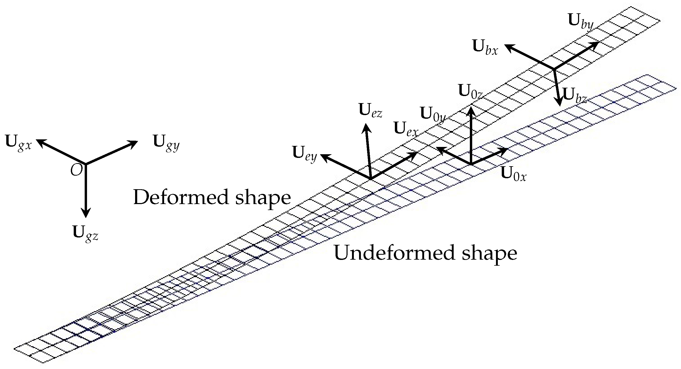
In the traditional flight dynamics, the aircraft is modeled as a rigid body with six degrees-of-freedom. However, due to the different velocities and orientation angles at different locations of the flexible aircraft, it is no longer proper to represent the aircraft as a rigid body. The Euler angles (roll, pitch and yaw angles) and airflow angles (angles of attack and sideslip) for a flexible aircraft should be redefined at the local element level.

In the present framework, given the spatial locations and orientations of every element, the ground, body and airflow axes for flight dynamics are re-defined analogously to the global and elemental reference frames for structural dynamics at the local element level.

As illustrated in Figure 2, the ground axes ${\mathbf{U}}_g$ for flight dynamics is defined to be identical to the global reference frame for aeroelasticity. For each element, there is a body-attached element frame ${\mathbf{U}}_e$, which translates and rotates continuously with the varying generalized displacements of the element. The element frame ${\mathbf{U}}_e$ in aeroelasticity is then taken as the body axes ${\mathbf{U}}_b$ for flight dynamics. Note that, according to the most usual practice in flight dynamics, the x axis of ${\mathbf{U}}_b$ is directed to “forward”, y axis to “rightward”, and z axis to “downward”, while, in aeroelasticity, the x axis of the element frame is preferred to lie along the axial line of the beam, and y and z axes along the principal axes of inertia. Thus, the body axes ${\mathbf{U}}_b$ of a wing element is defined as:

$${\mathbf{U}}_b=[{\mathbf{U}}_{ey},{\mathbf{U}}_{ex},-{\mathbf{U}}_{ez}]$$

(34)

where ${\mathbf{U}}_{ex}$, ${\mathbf{U}}_{ey}$ and ${\mathbf{U}}_{ez}$ are the base vectors of ${\mathbf{U}}_e$.

With ground axes ${\mathbf{U}}_g$ and elemental body axes ${\mathbf{U}}_b$ defined, the Euler angles (roll, pitch and yaw angles) of each element can be defined in the usual way. The translational velocity and acceleration of the element in body axes can be expressed as:

$${\mathbf{V}}_b={\mathbf{U}}_b^T{\mathbf{V}}_g;{\mathbf{a}}_b={\mathbf{U}}_b^T{\mathbf{a}}_g$$

(35)

where ${\mathbf{V}}_g$ and ${\mathbf{a}}_g$ are, respectively, the inertial velocity and acceleration vectors expressed in the ground or global axes.

The angular velocity and acceleration in body axes can be expressed as:

$$\mathbf{\omega }={[w_y,w_x,-w_z]}^T;\mathbf{\alpha }={[a_y,a_x,-a_z]}^T$$

(36)

where $w_x,w_y,w_z$ and $a_x,a_y,a_z$ are, respectively, the components of the elemental angular velocity and angular acceleration, which are defined in the element frame ${\mathbf{U}}_e$, in light of the co-rotational approach.

With the translational velocity in body axes, the angles of attack and sideslip of an element can be calculated as:

$$\alpha =arctan(V_{bz}/V_{bx});\beta =arcsin(V_{by}/V)$$

(37)

where $V_{bx}$, $V_{by}$ and $V_{bz}$ are the components of ${\mathbf{V}}_b$ and V is the norm of ${\mathbf{V}}_b$.

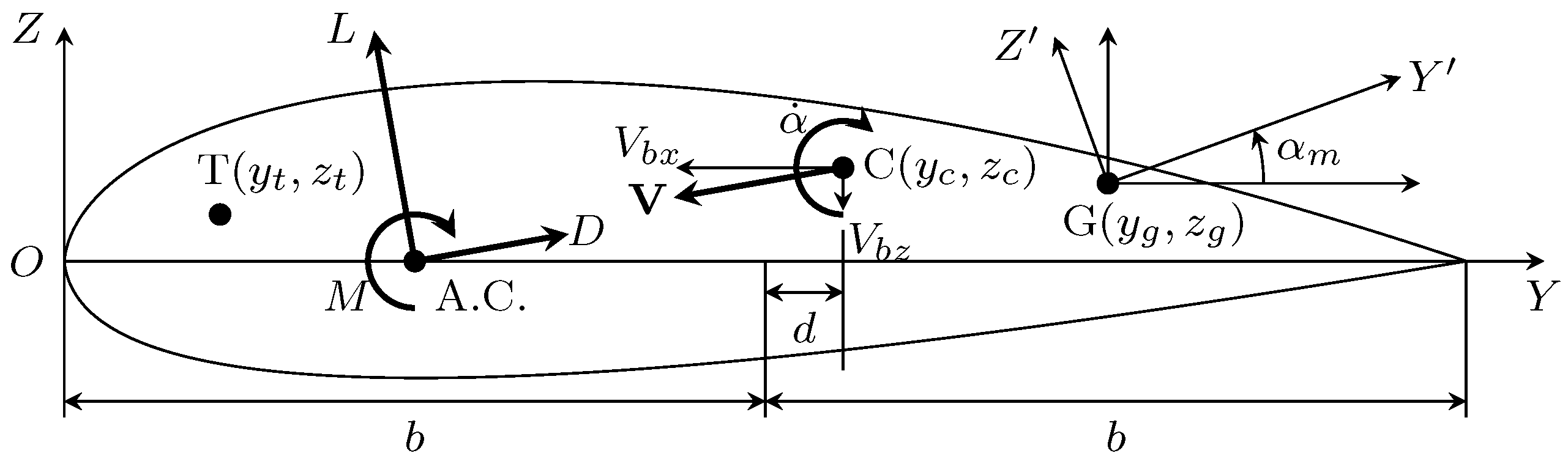
2.7. Peters’ Finite State Inflow Theory for Aerodynamic Modeling

The unsteady aerodynamic loads used in the current framework are based on the Peters’ 2D finite state inflow theory [45]. The model calculates aerodynamic loads on a thin airfoil section undergoing large motions in an incompressible flow. The aerodynamic loads per unit span calculated about the aerodynamic center (A.C.) are given as:

$$l_{ac}=\pi \rho b^2(\ddot{z}+\dot{y}\dot{\alpha }-d\ddot{\alpha })+c_{l\alpha }\rho b{\dot{y}}^2\left[\frac{\dot{z}}{\dot{y}}+(\frac{1}{2}b-d)\frac{\dot{\alpha }}{\dot{y}}-\frac{{\lambda }_0}{\dot{y}}\right]+\rho b{\dot{y}}^2(c_{l0}+c_{l\delta }\delta )$$

(38)

$$m_{ac}=-\pi \rho b^3\left[\frac{1}{2}\ddot{z}+\dot{y}\dot{\alpha }+(\frac{1}{8}b-\frac{1}{2}d)\ddot{\alpha }\right]+2\rho b^2{\dot{y}}^2(c_{m0}+c_{m\delta }\delta )$$

(39)

$$d_{ac}=\rho b{\dot{y}}^2{c}_{d0}$$

(40)

where $\rho$ is the air density, b is the semichord, d is the distance of the mid-chord in front of the reference axis (here, it is the shear center (C)), and $\delta$ is the trailing-edge flap deflection angle. $c_{l\alpha }$ is the lift curve slope and $c_{l\delta }$ and $c_{m\delta }$ are the lift and moment slopes due to flap deflection, respectively. $c_{l0}$, $c_{m0}$ and $c_{d0}$ are the lift, moment and drag coefficients for zero angle of attack (AOA), respectively. Furthermore, ${\lambda }_0$ is the inflow parameter, which accounts for induced flow due to free vorticity.

$${\lambda }_0=\frac{1}{2}{\mathbf{b}}^T\mathbf{\lambda }$$

(41)

where $\mathbf{\lambda }$ is the vector of inflow states [45], which is given by:

$$\mathbf{A}\dot{\mathbf{\lambda }}+\frac{\dot{y}}{b}\mathbf{\lambda }=\mathbf{c}[\ddot{z}+\dot{y}\dot{\alpha }+b(\frac{1}{2}-d)\ddot{\alpha }]$$

(42)

where $\mathbf{A}$, $\mathbf{b}$ and $\mathbf{c}$ are constants given as:

$$\begin{array}{cc}\hfill \mathbf{A}& =\mathbf{D}+\mathbf{d}{\mathbf{b}}^T+\mathbf{c}{\mathbf{d}}^T+\frac{1}{2}\mathbf{c}{\mathbf{b}}^T{b}_i={(-1)}^{i-1}\frac{(N+i)!}{(N-i)!}\frac{1}{{(i!)}^2}{c}_i=\frac{2}{i}\hfill \\ \hfill d_1& =0d_i=\frac{1}{2}(i\ne 1)D_{ij}=\frac{1}{2i}(i=j+1)D_{ij}=-\frac{1}{2i}(i=j-1);D_{ij}=0(i\ne j\pm 1)\hfill \end{array}$$

where N is the number of finite states.

To transfer the loads from A.C. to the wing reference axis (here, it is shear center (C)), one may use

$$l_{ra}=l_{ac};m_{ra}=m_{ac}+(\frac{1}{2}b+d)l_{ac};d_{ra}=d_{ac}$$

(43)

Furthermore, the aerodynamic loads are rotated to the body coordinate system, and then the global coordinate system, which yields:

$${\mathbf{F}}_a={\mathbf{U}}_e\left[\begin{array}{ccc}cos\left(\alpha \right)& 0& -sin\left(\alpha \right)\\ 0& 1& 0\\ sin\left(\alpha \right)& 0& cos\left(\alpha \right)\end{array}\right]\left[\begin{array}{ccc}cos\left(\beta \right)& sin\left(\beta \right)& 0\\ -sin\left(\beta \right)& cos\left(\beta \right)& 0\\ 0& 0& 1\end{array}\right]\left[\begin{array}{c}-d_{ra}\\ 0\\ -l_{ra}\end{array}\right]l$$

(44)

$${\mathbf{M}}_a={\mathbf{U}}_e\left[\begin{array}{ccc}cos\left(\alpha \right)& 0& -sin\left(\alpha \right)\\ 0& 1& 0\\ sin\left(\alpha \right)& 0& cos\left(\alpha \right)\end{array}\right]\left[\begin{array}{ccc}cos\left(\beta \right)& sin\left(\beta \right)& 0\\ -sin\left(\beta \right)& cos\left(\beta \right)& 0\\ 0& 0& 1\end{array}\right]\left[\begin{array}{c}0\\ m_{ra}\\ 0\end{array}\right]l$$

(45)

where l is the local span, which is here the length of the corresponding element.

Finally, the elemental force and moment are allocated equally to the two nodes of each element.

2.8. Nonlinear Trim of the Flexible Aircraft

The nonlinear trim of the flexible aircraft is performed for zero resultant force and moment of the whole aircraft. A cost function is defined as:

$$f={[{\mathbf{F}}_R^T,{\mathbf{M}}_R^T]}^T$$

(46)

where ${\mathbf{F}}_R$ and ${\mathbf{M}}_R$ are the resultant force and moment of the whole aircraft, which can be expressed as:

$${\mathbf{F}}_R=\sum _{i=1}^N{\mathbf{F}}_{ai}+\sum _{i=1}^N{\mathbf{F}}_{ti}+\sum _{i=1}^N{\mathbf{F}}_{gi}$$

(47)

$${\mathbf{M}}_R=\sum _{i=1}^N{\mathbf{M}}_{ai}+\sum _{i=1}^N{\mathbf{d}}_i\times ({\mathbf{F}}_{ai}+{\mathbf{F}}_{ti}+{\mathbf{F}}_{gi})$$

(48)

where ${\mathbf{F}}_{ai}$, ${\mathbf{M}}_{ai}$, ${\mathbf{F}}_{ti}$ and ${\mathbf{F}}_{gi}$ are, respectively, the aerodynamic force and moment, thrust and gravity acting on the ith node of the aircraft, and ${\mathbf{d}}_i$ is the distance vector from the moment reference point (e.g., center of gravity or the constraint point of the aircraft) to the ith node.

The cost function f is minimized over the solution space using the body angle of attack $\alpha$, elevator deflection angle $\delta$ and thrust T. Newton–Raphson iteration is employed to find the optimal trim parameter S, i.e.,

$$S_{k+1}=S_k-{\left[\frac{\partial f}{\partial S}\right]}_k^{-1}{f}_k$$

(49)

where $S={[\alpha ,\delta ,T]}^T$ and $\left[\frac{\partial f}{\partial S}\right]$ is the Jacobian matrix that relates the resultant force and moment of the whole aircraft with the trim parameters, which is computed numerically trough finite differences as:

$${\mathbf{J}}_{ij}\equiv \left[\frac{\partial f_i}{\partial S_j}\right]\simeq \frac{f_i(S+\Delta S_j)-f_i\left(S\right)}{\Delta S_j}$$

(50)

It is worth pointing out that, theoretically, Equation (49) is at risk of falling into a local minimum, but this situation is never seen to happen in practical applications.

3. Numerical Validation

Validations of the structural static solution under given loads and static aeroelastic responses with different flight conditions are presented in the previous work of the authors [35,36] and are not repeated here. To validate the implementation of the present framework and the corresponding computing codes, the dynamic responses of two representative numerical benchmarks, namely the cantilevered wing proposed by Goland [46] and the highly flexible flying wing proposed by Patil et al. [17], were analyzed and compared carefully to the results taken from Murua [22], Patil [17] and Su [13].

3.1. Cantilevered Goland Wing with Inertial Coupling

The cantilevered Goland wing was analyzed as a method-verification study for the present time-marching aeroelastic approach and the coupling of bending and torsional inertia. The properties of the Goland wing are given in

Table 3. Properties of Goland wing.

Property	Value	Property	Value
Span	6.096 m	Torsional stiffness	$9.87581\times {10}^5$ Nm${}^2$
Chord	1.8288 m	Bending stiffness	$9.77221\times {10}^6$ Nm${}^2$
Elastic axis	33% chord from L.E.	Chordwise bending stiffness	$9.77221\times {10}^6$ Nm${}^2$
Center of gravity	43% chord from L.E.	Mass per unit length	35.709121 kg/m
Air density	1.020 kg/m${}^3$	Mass moment of inertia about x axis	8.6405832 kgm

. With the effects of gravity neglected, the wing starts from rest with a very small AOA of 0.05 degree. The flutter speed was estimated in the time domain with different freestream velocities evaluated until the flutter onset was found.

Time histories of the wing-tip deflection and the corresponding torsional angle at three distinctive freestream velocities of 131.4, 136.4 and 141.4 m/s are plotted in Figure 3 and Figure 4, which, respectively, correspond to the damped, neutral and divergent states.

At the air speed of 131.4 m/s, the amplitude of oscillation decays and finally approaches to a steady state. As the air speed goes up to 136.4 m/s, a periodic motion with unchanged amplitude occurs, indicating the flutter speed is 136.4 m/s. The flutter frequency was calculated to be 69.2 rad/s, with a time-domain peak-finding technique. Above this speed, the wing oscillation tends to grow.

Table 4. Flutter speed and frequency of the Goland wing.

Author	Model	${\mathit{V}}_{\mathit{f}}$, m/s	${\mathit{\omega }}_{\mathit{f}}$, rad/s
Present	Co-rotational beam + strip theory	136.4	69.2
Goland [47]	Analytical	137.2	70.7
Patil et al. [48]	Intrinsic beam + strip theory	135.6	70.2
Murua [22]	Displacement beam + UVLM	165	69
Wang et al. [49]	Intrinsic beam + UVLM	163.8	-
Wang et al. [49]	ZAERO${}^{\copyright }$	174.3	-

compares the flutter speed and frequency obtained in the present framework to the results found in the literature. It can be seen that the flutter frequencies calculated with different models are almost the same, but the flutter speeds calculated with strip theory are approximately 18% lower than those with unsteady vortex lattice method (UVLM). This is because the two-dimensional strip theory cannot simulate the loss of lift near the tip of a wing with finite span, while the three-dimensional vortex lattice method can. Different from high aspect-ratio wings, the Goland wing has an aspect-ratio of only 3.33, in which the 3D effect cannot be neglected. Using the strip theory to calculate the flutter speed of 3D finite-span wings may result in underestimation.

To use 2D theory for a 3D wing, a spanwise distribution coefficient was applied to correct for the tip loss of lift:

$$C_{corr}=1-e^{-\tau s}(0\le s\le 1,\tau >1)$$

(51)

where $\tau$ is a user-defined parameter that controls the spanwise lift distribution and s is the distance between wingtip and the spanwise location of interest.

Despite the difference from 3D UVLM, excellent agreement with other models based on strip theory is reached, from which the sufficient accuracy of the established framework and its corresponding computing codes can be observed.

3.2. Flying Wing with Coupled Flight Dynamics and Aeroelasticity

To validate the implementation of the coupling of flight dynamics with nonlinear aeroelasticity and the corresponding computing codes, the trim and dynamic responses of a representative highly flexible flying-wing aircraft with a span of 72.8 m, a constant chord of 2.44 m and a payload varying from 0 to 227 kg on the central pod (note that the payload is not considered the entire mass at the point where the central pod locates; apart from the payload, there is also the structural mass of the central pod itself, which is 27.23 kg), as shown in Figure 5 and

Table 5. Properties of the flying wing (after [13]).

Strucutral Property	Value	Aerodynamic Property	Value
Cross-sectional elastic axis	25% chord from L.E.	$c_{l\alpha }$ for wings (25% chord)	2$\pi$
Cross-sectional center of gravity	25% chord from L.E.	$c_{l\delta }$ for wings (25% chord)	1
Torsional stiffness	$1.65301\times {10}^5$ Nm${}^2$	$c_{d0}$ for wings (25% chord)	0.01
Bending stiffness	$1.03313\times {10}^6$ Nm${}^2$	$c_{m0}$ for wings (25% chord)	0.025
Chordwise bending stiffness	$1.23976\times {10}^7$ Nm${}^2$	$c_{m\delta }$ for wings (25% chord)	−0.25
Mass per unit length	8.92898 kg/m	$c_{l\alpha }$ for pods (25% chord)	5
Torsional mass moment of inertia	4.14765 kgm	$c_{d0}$ for pods (25% chord)	0.02
Flatwise bending mass moment of inertia	0.691275 kgm
Chordwise bending mass moment of inertia	3.45637 kgm

, were analyzed and compared carefully to the results taken from Patil [17] and Su [13], respectively.

3.2.1. Trim Analysis

At the flight speed of 12.2 m/s at sea level, the highly flexible aircraft with the varying concentrated payload was trimmed for zero resultant force and moment. Figure 6 shows the variations of the trimmed AOA, flap deflection angle (assuming constant throughout the span) and thrust per motor with the varying payload. It can be seen that the trim AOA increases with the payload, as the heavier is the payload, the higher is the lift required, and thus the higher are the AOAs. When the concentrated payload increases, the aerodynamic loads get higher, which leads to large bending deformations in the highly flexible wings, and the aircraft turns into a “U” shape, as illustrated in Figure 7.

As the aircraft deforms to a “U” shape, the aerodynamic center moves backward, which brings about a pitch-down moment, and the flap deflection decreases to reduce the additional pitch-down moment of the flap. It can also be seen that the trimmed thrust does not change significantly with the payload. This phenomenon can be attributed to the simplicity of the drag model, in which the profile drag and frictional drag of the aircraft are constant and the induced drag that is proportional to the lift is not considered.

3.2.2. Effects of Structural Model and Mass Distribution on Trim

Figure 8 and Figure 9 show, respectively, the trimmed configurations, AOAs and flap deflection angles obtained with different structural models and different payload distributions. It can be seen that, for the concentrated payload located at the central pod, results from rigid, linear and nonlinear structural models are quite different. The rigid model keeps its initial shape, while the AOA increases and the flap deflection decreases linearly with the payload.

The difference in trimmed AOAs between linear and rigid structural models is brought by the aeroelastic deformation, especially the torsional deformations. Under the aerodynamic loads, the wings bend upward and twist positively, i.e., nose-up. With the positive torsion, a lower AOA is sufficient to provide the required lift, thus the linear model shows a lower AOA compared to the rigid one. On the other hand, as a follower force, the local lift is always perpendicular to the airfoil, with the directions changing continuously with the deformed configurations of the wing, so that it no longer acts in the vertical direction. Large bending deflections and the associated loss of vertical lift lead to the requirement of a higher AOA. This is the main reason the AOAs from the nonlinear model are higher than those from the rigid one when the payload exceeds 160 kg.

Furthermore, it can also be seen in Figure 7 that the bending deflection at wingtip of the nonlinear structural model is about 53% larger than that of the linear one, which indicates higher loss of lift, and results in a higher AOA, as illustrated in Figure 8.

The flap is mainly used to balance the pitch moment. Since there are no deformations, the flap deflection of rigid model decreases linearly with the payload as a result of the increasing pitch-down moment brought by the increasing AOA. The nonlinear structural model has larger deformations than the linear one, resulting in a larger back-shift of the aerodynamic center and larger pitch-down moment, and the flap deflections are much lower than those given by the linear structural model, as shown in Figure 9.

In Figure 7, we can see that, if the payload is concentrated on the central pod, the flexible aircraft will perform a highly deformed “U” shape configuration, leading to the dramatic changes in its trim and further in flight dynamic performances. If we now spread the payload equally to the three pods, there will be an almost evenly distributed mass that is balanced by the lift, and the deformations will be nearly negligible even with the heaviest payload. The variations of trim AOA and flap deflection angle of a highly flexible aircraft will behave almost as a rigid one, despite the slight differences that are mainly brought by the torsional deformations, as shown in Figure 8 and Figure 9.

Given the trim parameters and the deformed configurations, the aerodynamic characteristics, static and dynamic stabilities of the aircraft at each trimmed condition can be assessed accordingly, which are the topics of static aeroelasticity, and related studies were done in the previous works of the authors [35,36]. In addition, the comparison in Figure 6 shows excellent agreement with results from Patil [17] and Su [13], indicating the static aeroelastic characteristics of the flying wing calculated here are sufficiently accurate.

3.2.3. Stability Analysis

Time-domain simulations of the nonlinear dynamic responses of the highly flexible aircraft with three different payload masses (122, 152 and 227 kg) were performed. The aircraft was initially at its trimmed state, and perturbation was introduced by adding a pre-defined flap deflection change: the flap deflection angle was ramped linearly up to 5° between 1 and 2 s, then ramped linearly back to its trimmed angle between 2 and 3 s, and finally kept constant.

The simulation was conducted by the direct solution of the complete nonlinear dynamic equations by implicit predictor–corrector schemes with the mixed time-marching algorithms and a time step of up to 0.1 s. Figure 10, Figure 11 and Figure 12 show the variations of altitude, airspeed and AOA of the mid-span (the center) of the aircraft, respectively.

It can be seen in Figure 10 and Figure 11 that, with a payload of 122 kg at the central pod, the phugoid mode of the highly flexible aircraft is neutrally stable, as the altitude and airspeed of the vehicle after perturbation oscillate with equal amplitudes. When the payload increases to 152 or 227 kg, the phugoid mode becomes unstable with increasing amplitudes of oscillations: the heavier is the payload, the higher is the frequency and the larger is the amplitude of the oscillation. For the differences between the two results given by Patil [17] and Su [13], Su attributed them to the differences of damping of the models used, which the authors think was not explained precisely. In the opinion of the authors of the present paper, it is more likely to be the difference of payload masses that leads to the different results.

In Figure 10 and Figure 11, the exchange between potential energy and kinetic energy of the highly flexible aircraft can be seen clearly from the out-of-phase variations between the altitudes and airspeeds. Besides, the aircraft altitude loss indicates a loss of energy due to the unstable phugoid mode and constant thrust.

As shown in Figure 12, within several cycles of oscillations, the mid-span (also the whole aircraft) starts to experience very high AOAs in every cycle, which is the inevitable result of the excited unstable phugoid mode.

It is to be noted that, since stall is not yet included in the present framework, the results at high AOAs cannot be considered to be the real motion of the aircraft. Once the dynamic stall is included, one would see the different responses at the highest altitudes, where the lift will be insufficient to balance the weight and the aircraft drops with the increase in velocity, resulting in instantaneous higher AOAs.

In addition, it can be clearly seen that excellent agreements are made with the results supplied by Patil [17] for 227 kg payload mass and Su [13] for 152 kg payload mass, which demonstrates the validity and accuracy of the presented framework and its corresponding computing codes.

3.2.4. Effects of Mass Distribution on Longitudinal Stability

It is known from the results and analyses presented in Section 3.2.1 that the spanwise distribution of mass will affect the trimmed state of the aircraft, which will further influence the flight dynamic characteristics. It can be inferred that the mass distribution in spanwise will alter the longitudinal stability, changing the unstable phugoid mode into a stable one.

In this experiment, part of the 152 kg payload remained in the central pod, and the remaining mass was distributed equally to the left and right ones.

Figure 13 shows the variations of the altitude of the mid-span of the highly flexible aircraft with, respectively, 100%, 95%, 90% and 80% of the total payload mass on the central pod and the rest on the side ones.

It can be clearly seen that, in the case of the same total payload, with the reduction of the mass at central pod, the amplitude of oscillation decreases dramatically; the frequency also decreases to some extent. When the mass on the central pod reduces to 80% of the total payload, the amplitude of oscillation after perturbation even begins to decay.

With the varying distributions of payload mass, other parameters (the airspeeds and AOAs) have the same trend as the altitude of the aircraft, which are not explain in details here. Generally, for a rigid straight wing without sweep and dihedral, the effects of spanwise mass distributions on longitudinal stability and dynamic responses are negligible. However, it clearly tells that the longitudinal stability and dynamic responses of a flexible wing will be significantly affected by the spanwise mass distributions. With the same mass of payload, a span-loaded aircraft is more stable than a center-loaded one.

4. Concluding Remarks

A new and comprehensive analytical framework for the coupled flight dynamics and nonlinear aeroelasticity of highly flexible aircrafts is presented. The theoretical methodology is based on the statics and dynamics of a 3D co-rotational geometrically nonlinear beam model for elastic deformations and rigid-body motions, with the original equations for nodal inertial force vector of element modified to enhance its versatility. The coupling of axial, bending and torsional effects is considered by adding the coupling terms into the element stiffness and mass matrices of traditional Euler–Bernoulli beam in order to capture the most relevant characteristics of real wing structure. The Peters’ finite-state unsteady aerodynamic model is coupled with the structural model to simulate the unsteady aerodynamics in flight. The flight dynamics are coupled with nonlinear aeroelasticity in a more intuitive and straightforward way by re-defining the ground, body and airflow axes analogously to the global and elemental reference frames for structural dynamics at the local element level, followed by the definitions of local Euler angles and airflow angles of each element. The scheme of mixed end-point and mid-point time-marching algorithm is proposed and applied into the implicit predictor–corrector integration for the first time, by which the computation efficiency, accuracy and stability are improved.

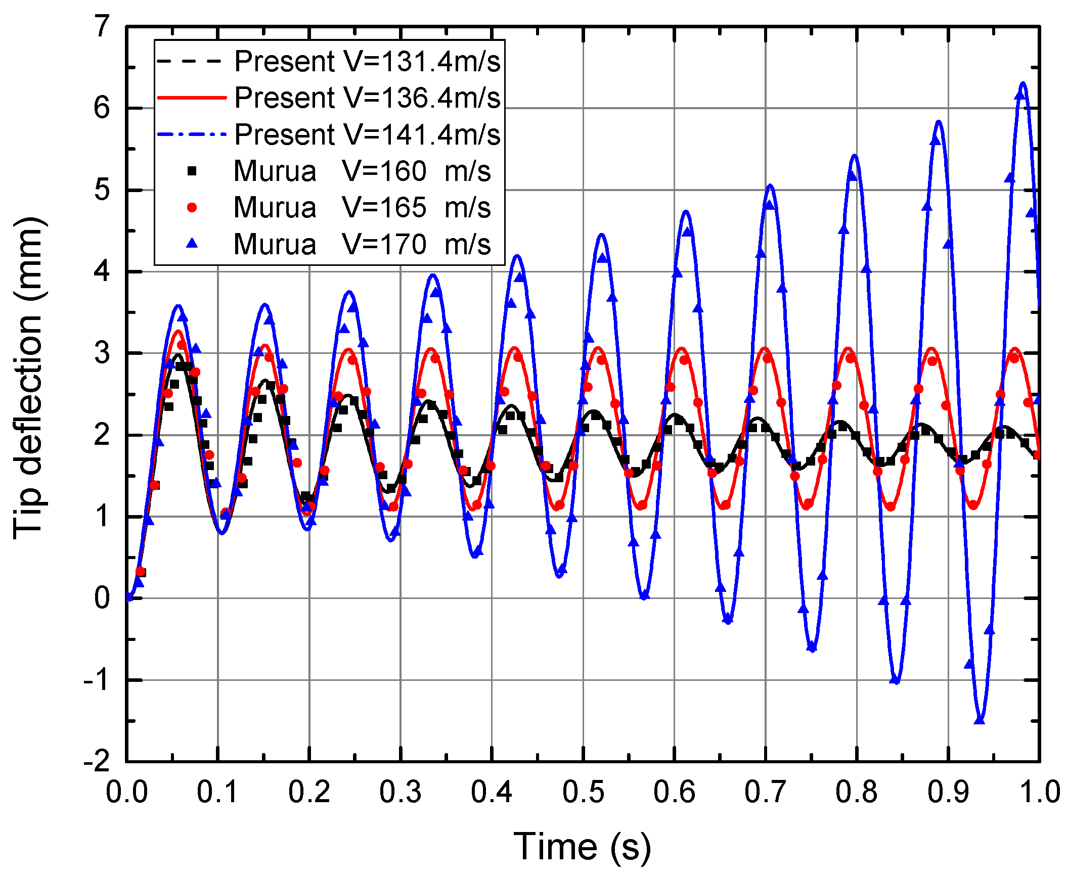
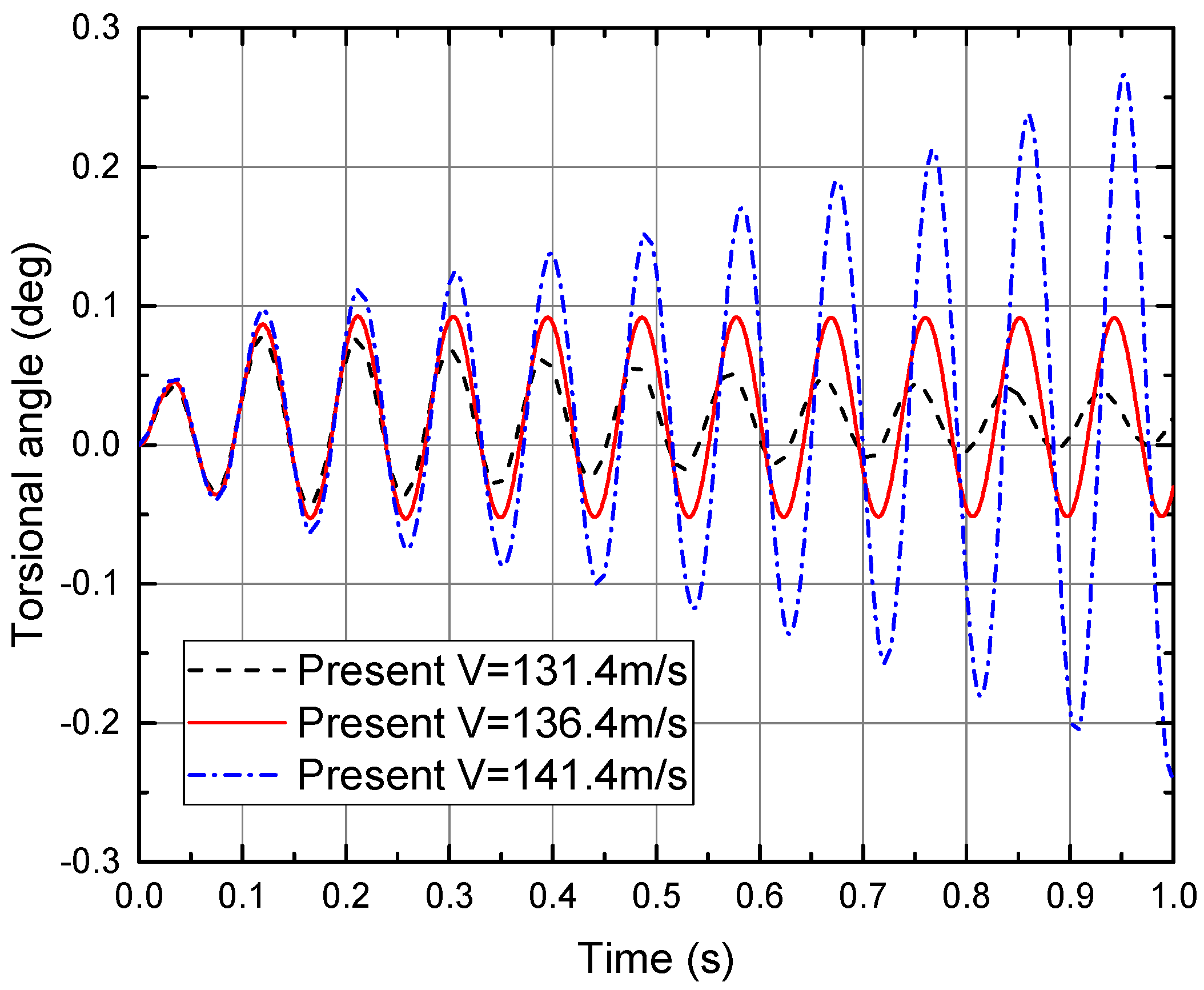
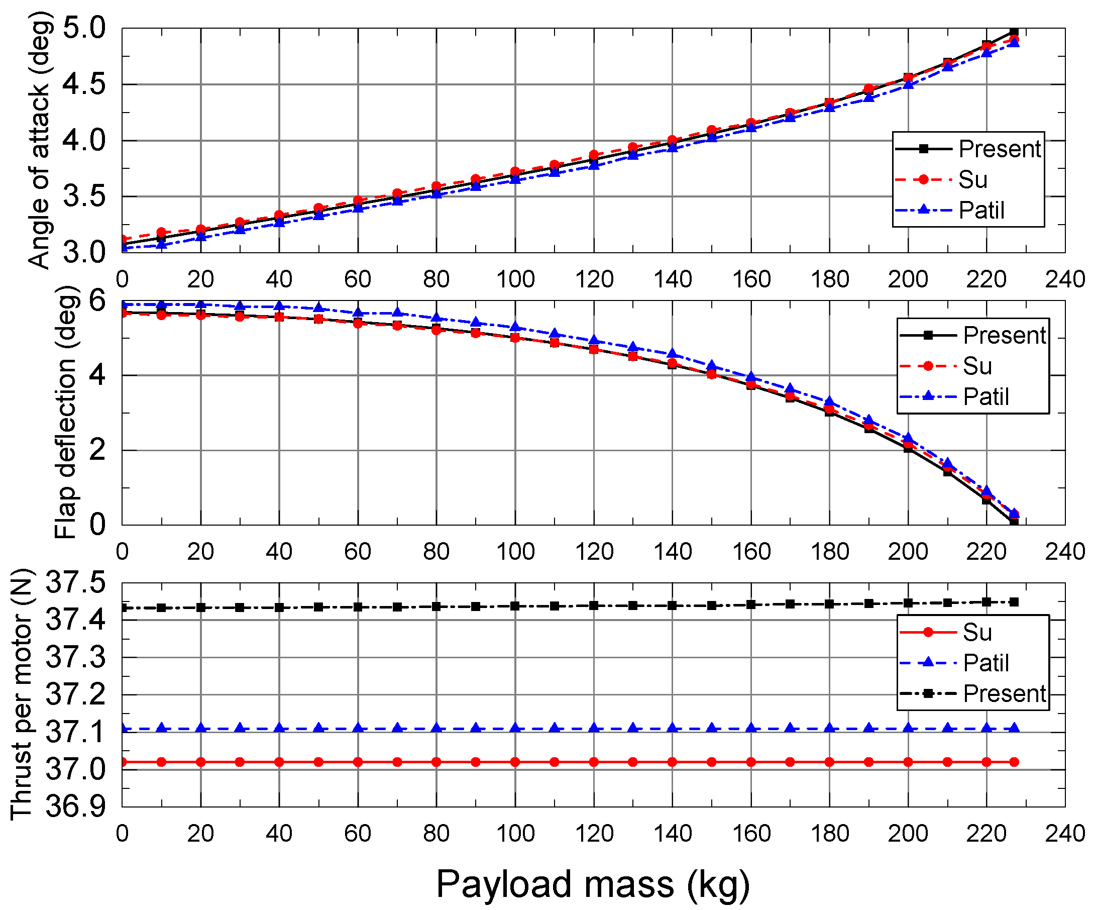
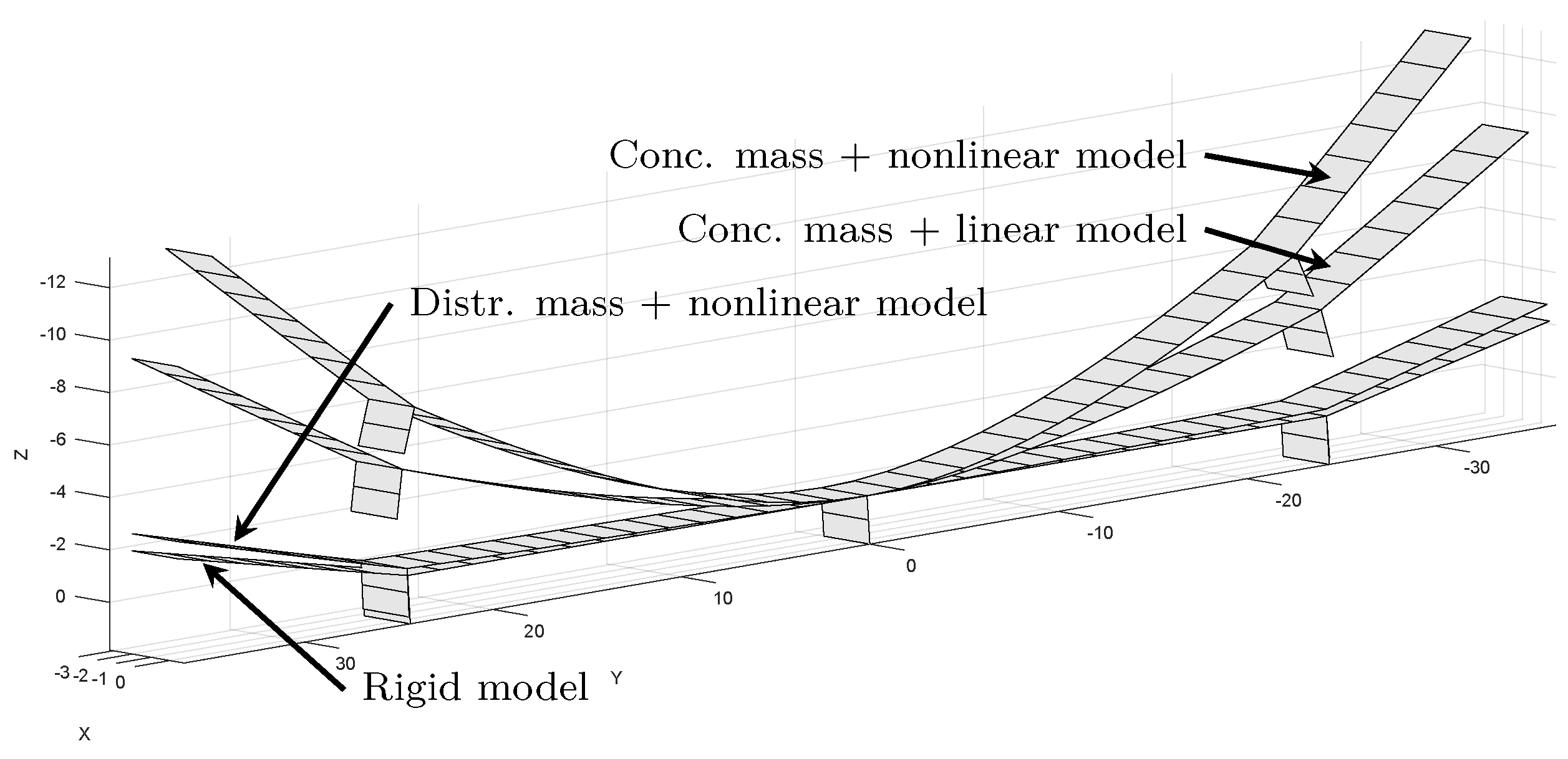
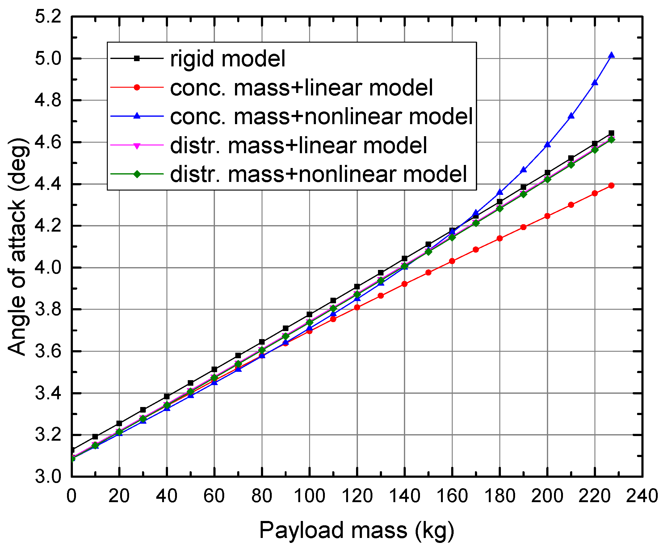
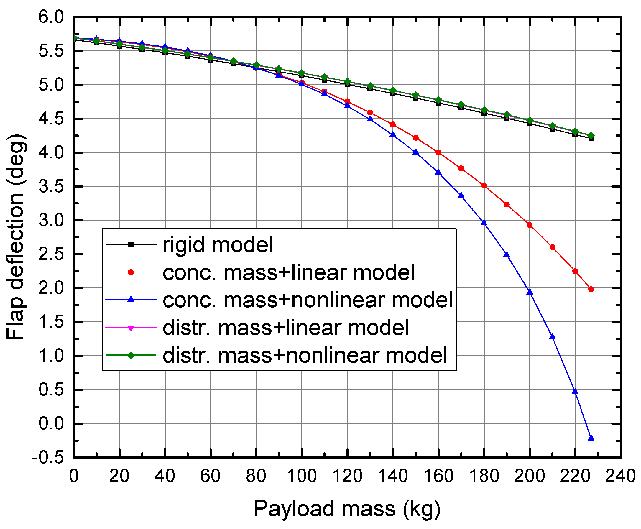
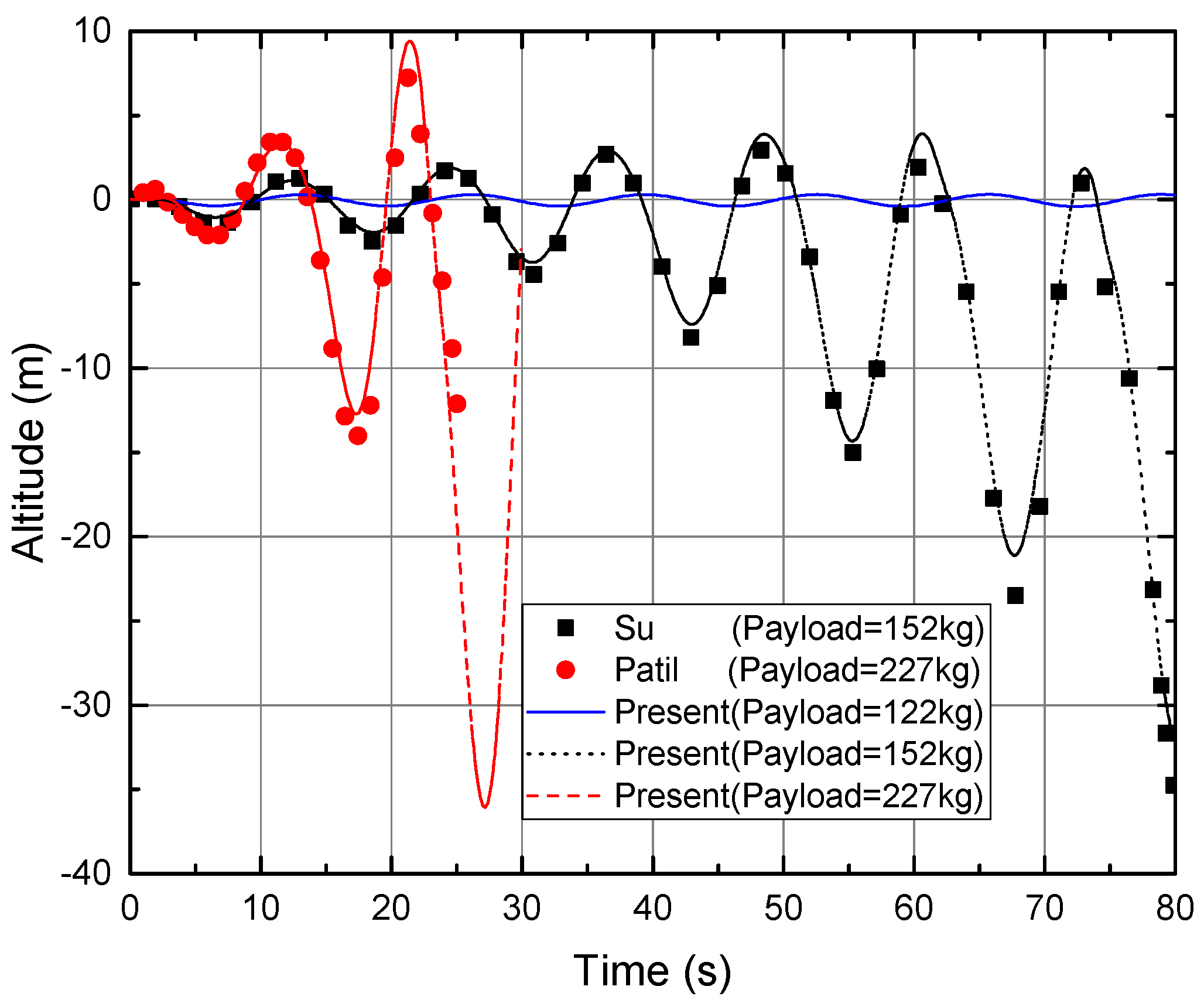
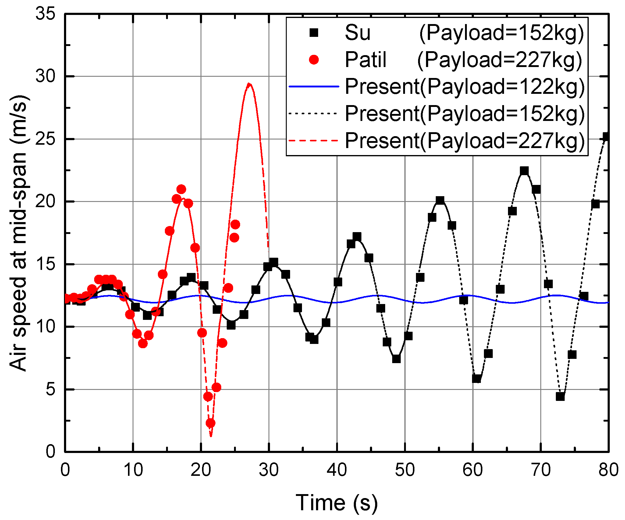
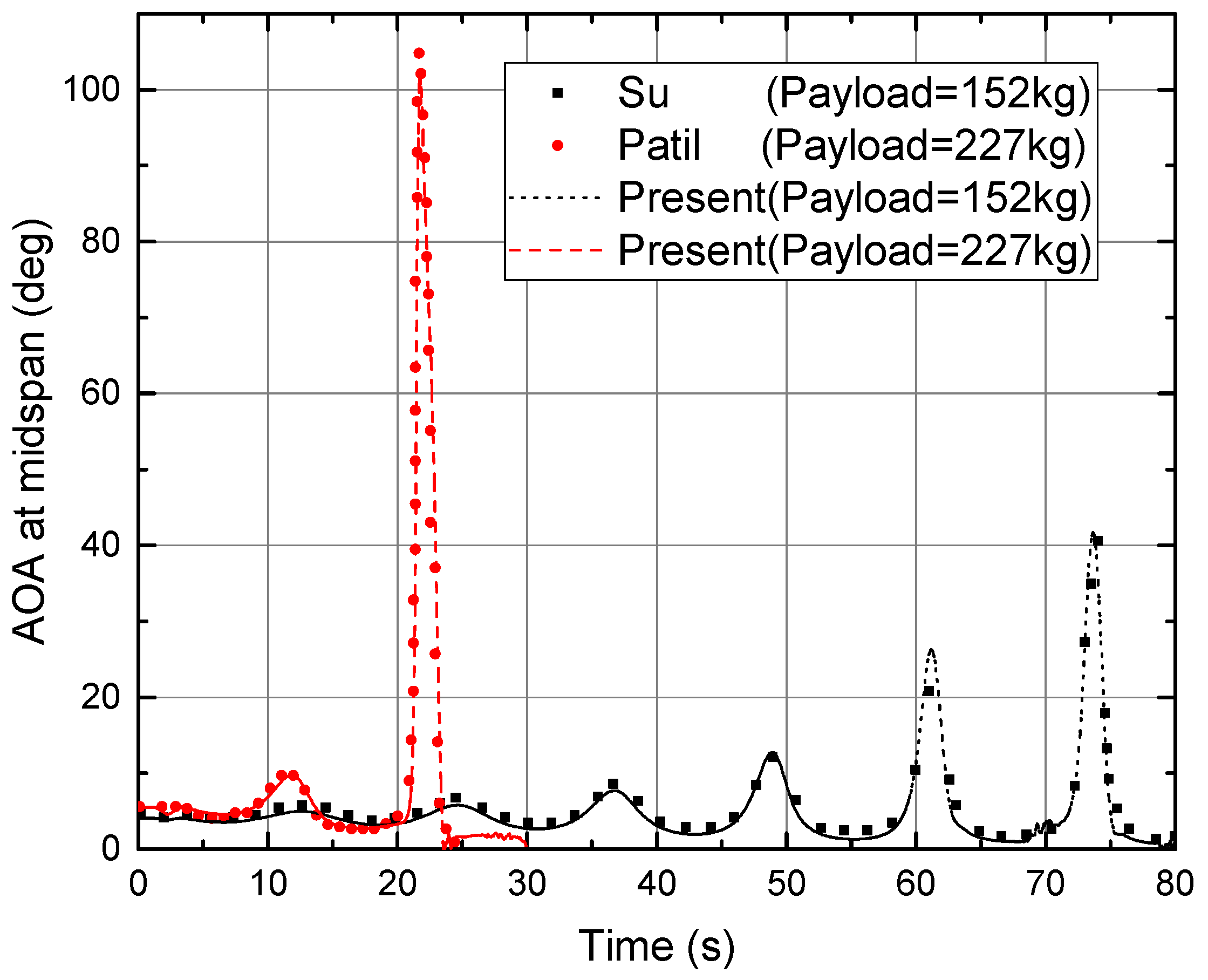
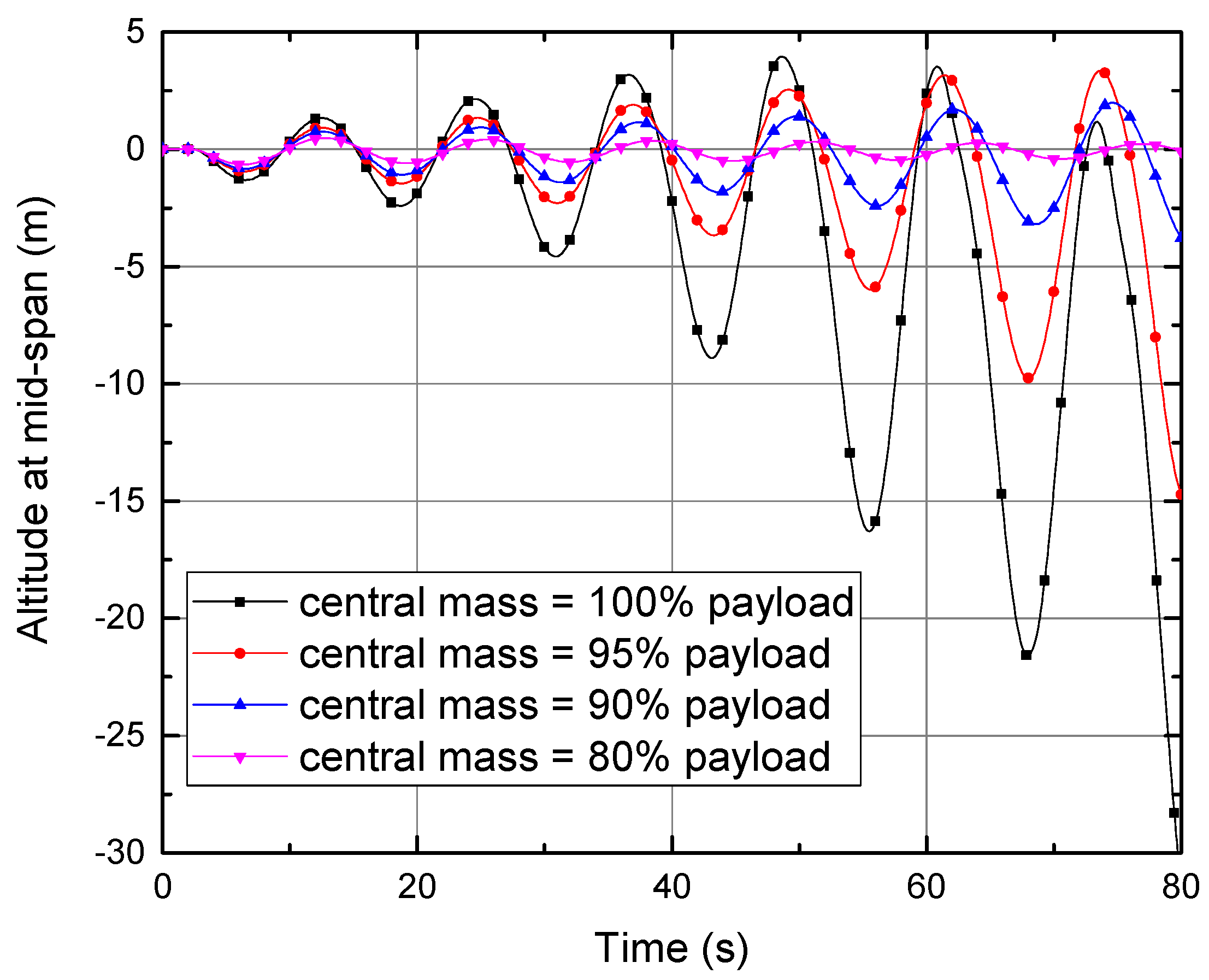
Two representative numerical benchmarks, especially a highly flexible flying-wing aircraft, are presented and analyzed with the trimmed states calculated and dynamic responses after flap perturbations computed numerically. The results show that with the increase of the concentrated payload, large deformations occur in the highly flexible wings, resulting in significant changes in trim state and the reduction in phugoid mode stability. The effects of spanwise mass distribution on trim and longitudinal stability are further studied, indicating that, for highly flexible aircrafts, the longitudinal performances will be affected by the spanwise mass distribution; span-loaded aircrafts with distributed payloads have much smaller deformations and higher longitudinal stabilities than the center-loaded ones with concentrated payloads.

The present framework accounts for realistic design elements including arbitrary structural shapes and properties, concentrated masses, multiple thrusts and control surfaces and unsteady aerodynamics. It is adaptive and easy to accommodate with other models, and can be used for complete aircraft analyses in the conceptual and preliminary design phases, including the quick linear and nonlinear trim, aerodynamic load estimation, stability assessment, as well as linear and nonlinear time-domain response simulations and further control evaluations. Comparisons with published literature show the validity and reliability of the present framework. The investigations on lateral and directional characteristics and symmetric and unsymmetrical gust responses with dynamic stall effects of large-scale flexible aircrafts based on the present framework will be the focus of the future work.

References

1. Gonzalo, J.; López, D.; Domínguez, D.; García, A.; Escapa, A. On the capabilities and limitations of high altitude pseudo-satellites. Prog. Aerosp. Sci. 2018, 98, 37–56. [Google Scholar] [CrossRef]
2. Noll, T.E.; Brown, J.M.; Perez-davis, M.E.; Ishmael, S.D.; Tiffany, G.C.; Gaier, M. Investigation of the Helios Prototype Aircraft Mishap; Technical Report January; NASA: Washington, DC, USA, 2004.
3. Modaress-Aval, A.H.; Bakhtiari-Nejad, F.; Dowell, E.H.; Peters, D.A.; Shahverdi, H. A comparative study of nonlinear aeroelastic models for high aspect ratio wings. J. Fluids Struct. 2019, 85, 249–274. [Google Scholar] [CrossRef]
4. Cesnik, C.E.; Palacios, R.; Reichenbach, E.Y. Reexamined structural design procedures for very flexible aircraft. J. Aircr. 2014, 51, 1580–1591. [Google Scholar] [CrossRef] [Green Version]
5. Wang, Y.; Wynn, A.; Palacios, R. Nonlinear Aeroelastic Control of Very Flexible Aircraft Using Model Updating. J. Aircr. 2018, 55, 1551–1563. [Google Scholar] [CrossRef]
6. Mardanpour, P.; Hodges, D.H.; Rezvani, R. Nonlinear aeroelasticity of high-aspect-ratio wings excited by time-dependent thrust. Nonlinear Dyn. 2014, 75, 475–500. [Google Scholar] [CrossRef]
7. Rezaei, M.M.; Behzad, M.; Haddadpour, H.; Moradi, H. Aeroelastic analysis of a rotating wind turbine blade using a geometrically exact formulation. Nonlinear Dyn. 2017, 89, 2367–2392. [Google Scholar] [CrossRef]
8. Shams, S.; Sadr, M.H.; Haddadpour, H. An efficient method for nonlinear aeroelasticy of slender wings. Nonlinear Dyn. 2012, 67, 659–681. [Google Scholar] [CrossRef]
9. Aliakbari, N.; Moeenfard, H. Analytical modeling of nonlinear vibrations in a 2-DOF airfoil device based on an unsteady flow model. Nonlinear Dyn. 2018, 91, 427–442. [Google Scholar] [CrossRef]
10. Chang, C.S.; Hodges, D.H.; Patil, M.J. Flight Dynamics of Highly Flexible Aircraft. J. Aircr. 2008, 45, 538–545. [Google Scholar] [CrossRef]
11. Nayfeh, A.H.; Ghommem, M.; Hajj, M.R. Normal form representation of the aeroelastic response of the Goland wing. Nonlinear Dyn. 2012, 67, 1847–1861. [Google Scholar] [CrossRef]
12. Shukla, H.; Patil, M.J. Nonlinear state feedback control design to eliminate subcritical limit cycle oscillations in aeroelastic systems. Nonlinear Dyn. 2017, 88, 1599–1614. [Google Scholar] [CrossRef]
13. Su, W..; Cesnik, C.E.S. Dynamic Response of Highly Flexible Flying Wings. AIAA J. 2011, 49, 324–339. [Google Scholar] [CrossRef]
14. Murua, J.; Palacios, R.; Graham, J.M.R. Applications of the unsteady vortex-lattice method in aircraft aeroelasticity and flight dynamics. Prog. Aerosp. Sci. 2012, 55, 46–72. [Google Scholar] [CrossRef] [Green Version]
15. Wang, Z.; Chen, P.C.; Liu, D.D.; Mook, D.T. Nonlinear-aerodynamics/nonlinear-structure interaction methodology for a high-altitude long-endurance wing. J. Aircr. 2010, 47, 556–566. [Google Scholar] [CrossRef] [Green Version]
16. Patil, M.; Hodges, D.; Cesnik, C. Limit-Cycle Oscillations in High-Aspect-Ratio Wings. J. Fluids Struct. 2001, 15, 107–132. [Google Scholar] [CrossRef]
17. Patil, M.J.; Hodges, D.H. Flight Dynamics of Highly Flexible Flying Wings. J. Aircr. 2006, 43, 1790–1799. [Google Scholar] [CrossRef] [Green Version]
18. Cesnik, C.E.; Su, W. Nonlinear aeroelastic modeling and analysis of fully flexible aircraft. In Collection of Technical Papers—AIAA/ASME/ASCE/AHS/ASC Structures, Structural Dynamics and Materials Conference; American Institute of Aeronautics and Astronautics: Reston, VA, USA, 2005; Volume 7, pp. 4472–4498. [Google Scholar]
19. Shearer, C.M.; Cesnik, C.E. Nonlinear flight dynamics of very flexible aircraft. J. Aircr. 2007, 44, 1528–1545. [Google Scholar] [CrossRef] [Green Version]
20. Shearer, C.M.; Cesnik, C.E. Trajectory control for very flexible aircraft. J. Guid. Control Dyn. 2008, 31, 340–357. [Google Scholar] [CrossRef] [Green Version]
21. Hesse, H.; Palacios, R. Reduced-order aeroelastic models for dynamics of maneuvering flexible aircraft. AIAA J. 2014, 52, 1717–1732. [Google Scholar] [CrossRef]
22. Murua, J.; Palacios, R.; Graham, J.M.R. Assessment of Wake-Tail Interference Effects on the Dynamics of Flexible Aircraft. AIAA J. 2012, 50, 1575–1585. [Google Scholar] [CrossRef] [Green Version]
23. Borker, R.; Huang, D.; Grimberg, S.; Farhat, C.; Avery, P.; Rabinovitch, J. Mesh adaptation framework for embedded boundary methods for computational fluid dynamics and fluid-structure interaction. Int. J. Numer. Methods Fluids 2019, 90, 389–424. [Google Scholar] [CrossRef]
24. Grimberg, S.; Farhat, C. Fast computation of the wall distance in unsteady Eulerian fluid-structure computations. Int. J. Numer. Methods Fluids 2019, 89, 143–161. [Google Scholar] [CrossRef]
25. Huang, D.Z.; De Santis, D.; Farhat, C. A family of position-and orientation-independent embedded boundary methods for viscous flow and fluid–structure interaction problems. J. Comput. Phys. 2018, 365, 74–104. [Google Scholar] [CrossRef]
26. Wang, K.; Lea, P.; Farhat, C. A computational framework for the simulation of high-speed multi-material fluid–structure interaction problems with dynamic fracture. Int. J. Numer. Methods Eng. 2015, 104, 585–623. [Google Scholar] [CrossRef]
27. Farhat, C.; Rallu, A.; Wang, K.; Belytschko, T. Robust and provably second-order explicit–explicit and implicit–explicit staggered time-integrators for highly non-linear compressible fluid–structure interaction problems. Int. J. Numer. Methods Eng. 2010, 84, 73–107. [Google Scholar] [CrossRef]
28. Amsallem, D.; Farhat, C. Interpolation method for adapting reduced-order models and application to aeroelasticity. AIAA J. 2008, 46, 1803–1813. [Google Scholar] [CrossRef] [Green Version]
29. Lieu, T.; Farhat, C.; Lesoinne, M. Reduced-order fluid/structure modeling of a complete aircraft configuration. Comput. Methods Appl. Mech. Eng. 2006, 195, 5730–5742. [Google Scholar] [CrossRef]
30. Afonso, F.; Vale, J.; Oliveira, É.; Lau, F.; Suleman, A. A review on non-linear aeroelasticity of high aspect-ratio wings. Prog. Aerosp. Sci. 2017, 89, 40–57. [Google Scholar] [CrossRef]
31. Waszak, M.R.; Schmidt, D.K. Flight dynamics of aeroelastic vehicles. J. Aircr. 1988, 25, 563–571. [Google Scholar] [CrossRef]
32. Wu, Z.G.; Yang, C. Flight Loads and Dynamics of Flexible Air Vehicles. Chin. J. Aeronaut. 2004, 17, 17–22. [Google Scholar] [CrossRef] [Green Version]
33. Tang, D.; Dowell, E. Experimental and theoretical study on aeroelastic response of high-aspect-ratio wings. AIAA J. 2001, 39, 1430–1441. [Google Scholar] [CrossRef]
34. Larsen, J.W.; Nielsen, S.R.K.; Krenk, S. Dynamic stall model for wind turbine airfoils. J. Fluids Struct. 2007, 23, 959–982. [Google Scholar] [CrossRef]
35. Zhang, C.; Zhou, Z.; Meng, P. Nonlinear Static Aeroelastic and Trim Analysis of Highly Flexible Aircraft. In Proceedings of the 31st Congress of the International Cuncil of the Aeronautical Sciences, Belo Horizonte, Brazil, 9–14 September 2018. [Google Scholar]
36. Zhang, C.; Zhou, Z.; Zhu, X.; Meng, P. Nonlinear Static Aeroelastic and Trim Analysis of Highly Flexible Joined-Wing Aircraft. AIAA J. 2018, 56, 4988–4999. [Google Scholar] [CrossRef]
37. Crisfield, M.A.; Galvanetto, U.; Jelenić, G. Dynamics of 3-D co-rotational beams. Comput. Mech. 1997, 20, 507–519. [Google Scholar] [CrossRef]
38. Crisfield, M. Non-Linear Finite Element Analysis of Solids and Structures Volume 2: Advanced Topics; John Wiley & Sons: Hoboken, NJ, USA, 1997. [Google Scholar]
39. Crisfield, M.A. A consistent co-rotational formulation for non-linear, three-dimensional, beam-elements. Comput. Methods Appl. Mech. Eng. 1990, 81, 131–150. [Google Scholar] [CrossRef]
40. Chung, J.; Hulbert, G. A Time Integration Algorithm for Structural Dynamics with Improved Numerical Dissipation—The Generalized-alpha Method. J. Appl. Mech.-Trans. ASME 1993, 60, 371–375. [Google Scholar] [CrossRef]
41. Bathe, K.J.; Bolourchi, S. Large displacement analysis of three-dimensional beam structures. Int. J. Numer. Methods Eng. 1979, 14, 961–986. [Google Scholar] [CrossRef]
42. Cardona, A.; Geradin, M. A beam finite element non-linear theory with finite rotations. Int. J. Numer. Methods Eng. 1988, 26, 2403–2438. [Google Scholar] [CrossRef]
43. Crisfield, M.A.; Shi, J. An energy conserving co-rotational procedure for non-linear dynamics with finite elements. Nonlinear Dyn. 1996, 9, 37–52. [Google Scholar] [CrossRef]
44. De Frias Lopez, R. A 3D Finite Beam Element for the Modelling of Composite wind Turbine Wings. Master’s Thesis, KTH, Stockholm, Sweden, 2013. [Google Scholar]
45. Peters, D.A.; Karunamoorthy, S.; Cao, W.M. Finite state induced flow models. Part I: Two-dimensional thin airfoil. J. Aircr. 1995, 32, 313–322. [Google Scholar] [CrossRef]
46. Goland, M. The Flutter of a Uniform Cantilever Wing. J. Appl. Mech. 1945, 12, A197–A208. [Google Scholar]
47. Goland, M.; Luke, Y.L. The Flutter of a Uniform Cantilever Wing with Tip Weights. J. Appl. Mech. 1948, 15, 13–20. [Google Scholar]
48. Patil, M.J.; Hodges, D.H.; Cesnik, C.E.S. Nonlinear Aeroelastic Analysis of Complete Aircraft in Subsonic Flow. J. Aircr. 2000, 37, 753–760. [Google Scholar] [CrossRef] [Green Version]
49. Wang, Z.; Chen, P.C.; Liu, D.D.; Mook, D.T.; Patil, M.J. Time domain nonlinear aeroelastic analysis for HALE wings. In Collection of Technical Papers—AIAA/ASME/ASCE/AHS/ASC Structures, Structural Dynamics and Materials Conference; American Institute of Aeronautics and Astronautics: Reston, VA, USA, 2006; pp. 488–506. [Google Scholar]
Figure 1. Beam reference coordinate system.
Applsci 10 00949 g001
Figure 2. Global (ground), elemental and body reference frames of the flexible wing.
Applsci 10 00949 g002
Figure 3. Time history of Goland wing-tip deflection at various freestream velocities.
Applsci 10 00949 g003
Figure 4. Time history of Goland wing-tip torsional angle at various freestream velocities.
Applsci 10 00949 g004
Figure 5. Geometry of the flying wing model.
Applsci 10 00949 g005
Figure 6. Trim results of the flying wing with varying payload mass.
Applsci 10 00949 g006
Figure 7. Trimmed configurations of different models with heavy payload.
Applsci 10 00949 g007
Figure 8. Trim AOA the flying wing with different models.
Applsci 10 00949 g008
Figure 9. Flap deflection of the flying wing with different models.
Applsci 10 00949 g009
Figure 10. Altitude of flight with different payload.
Applsci 10 00949 g010
Figure 11. Airspeed of flight with different payload.
Applsci 10 00949 g011
Figure 12. AOA at mid-span with different payload.
Applsci 10 00949 g012
Figure 13. Altitude at mid-span with the same weight but different payload distributions.
Applsci 10 00949 g013