Real-Time Haze Removal Using Normalised Pixel-Wise Dark-Channel Prior and Robust Atmospheric-Light Estimation

Abstract

This study proposes real-time haze removal from a single image using normalised pixel-wise dark-channel prior (DCP). DCP assumes that at least one RGB colour channel within most local patches in a haze-free image has a low-intensity value. Since the spatial resolution of the transmission map depends on the patch size and it loses the detailed structure with large patch sizes, original work refines the transmission map using an image-matting technique. However, it requires high computational cost and is not adequate for real-time application. To solve these problems, we use normalised pixel-wise haze estimation without losing the detailed structure of the transmission map. This study also proposes robust atmospheric-light estimation using a coarse-to-fine search strategy and down-sampled haze estimation for acceleration. Experiments with actual and simulated haze images showed that the proposed method achieves real-time results of visually and quantitatively acceptable quality compared with other conventional methods of haze removal.

1. Introduction

In recent years, self-driving vehicles, underwater robots, and remote sensing have attracted attention; such applications employ fast and robust image-recognition techniques. However, images of outdoor or underwater scenes have poor image quality because of haze (Figure 1a), thus affecting image recognition. To solve this problem, many haze removal techniques were proposed, and these techniques can be classified into non-learning-based and learning-based approaches.

Non-learning-based approaches use multiple haze images [1], depth information [2] and prior knowledge from a single haze image [3,4,5]. Methods employing prior knowledge maximise contrast within the local patch [3], assuming that surface shading and transmission are locally uncorrelated [4], and statistically observe that at least one RGB colour channel within most local patches in a haze-free image has a low-intensity value [5]. Median and guided-image filters [6,7] are used for accelerating haze removal; however, these methods could not achieve real-time processing (defined as 20 fps for our calculations herein). Learning-based approaches employ random forest [8], colour-attenuation and prior-based brightness-saturation relation [9] and deep learning [10,11]. These methods can achieve accurate and fast haze removal compared with conventional non-learning-based approaches. In deep-learning-based methods, large-scale pairs of haze images and corresponding haze-free images must be prepared and their relation must be trained. Image pairs of haze and haze-free images cannot be existed simultaneously in actual situation; therefore, haze images are generated from haze-free images by employing haze-observation model [10] and depth information from the corresponding haze-free images [11]. The haze-removal accuracy of deep-learning-based methods depends on the dataset and preparing large datasets is cumbersome. Deep-learning-based methods [10,11] are faster than conventional methods [5,6]; however, computational times of 1.5 s [10] and 0.61 s [11] are required for haze removal of a $640\times 480$ image using 3.4 GHz CPU without GPU acceleration; these methods also could not achieve real-time processing.

This study proposes a real-time haze-removal method using a normalised pixel-wise dark-channel prior (DCP) to enable real-time application (Figure 1b,c). This paper is an extended version of [12]. Contributions of the proposed method are as follows:

(a) 

Normalised pixel-wise DCP

Original patch-wise DCP method requires high computational cost to refine the transmission map using an image-matting technique. In this paper, we propose a normalised pixel-wise DCP method with no need for refinement of transmission map compared with the patch-wise method.

(b) 

Accelerating haze removal via down-sampling

We estimate the transmission map and atmospheric light using down-sampled haze image for acceleration. This idea is inspired by [13].

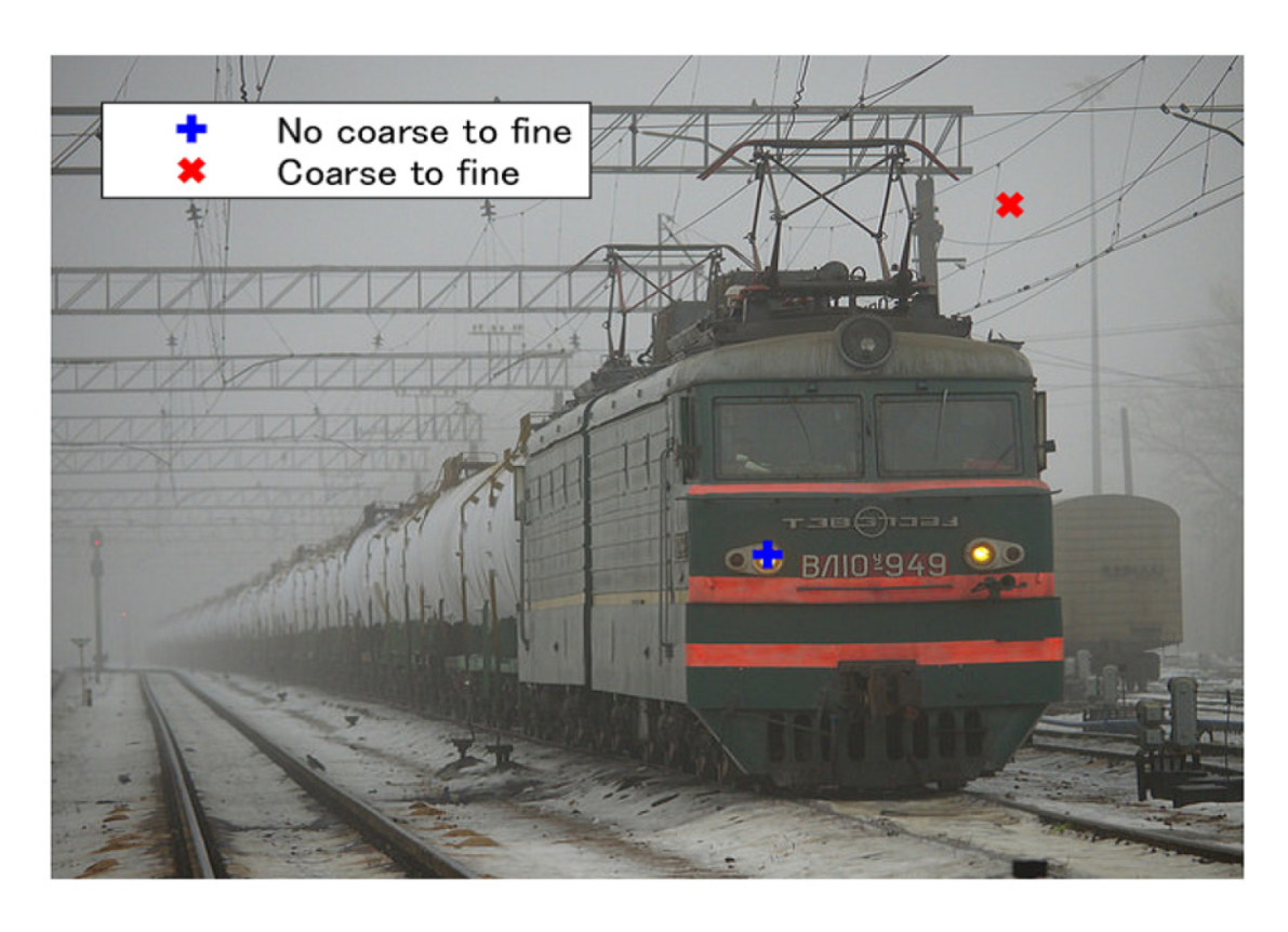
(c) 

Robust atmospheric-light estimation

To reduce the computational time and improve robustness, we propose a coarse-to-fine search strategy for atmospheric-light estimation.

The remainder of this paper is organized as follows. In Section 2, we introduces He et al.’s method [5] in detail because it forms the basis of the proposed method. Section 3 provides the description of proposed method. The experimental results and discussion are reported in Section 4, and conclusion is drawn in Section 5.

2. Traditional Dark Channel Prior

This section describes DCP [5], which is the basis of the proposed method. The haze-observation model [1,5] is represented by

$$\mathbf{I}\left(\mathbf{x}\right)=t\left(\mathbf{x}\right)\mathbf{J}\left(\mathbf{x}\right)+(1-t(\mathbf{x}\left)\right)\mathbf{A},$$

(1)

where $\mathbf{I}\left(\mathbf{x}\right)$ is the observed RGB colour vector of haze image at coordinate $\mathbf{x}$, $\mathbf{J}\left(\mathbf{x}\right)$ is the ideal haze-free image at coordinate $\mathbf{x}$, $\mathbf{A}$ is the atmospheric light, $t\left(\mathbf{x}\right)$ is the value of transmission map at coordinate $\mathbf{x}$. To solve the haze-removal problem, some prior knowledge such as DCP must be applied. The transmission map derivation (Section 2.1), atmospheric-light estimation (Section 2.2) and haze-removal image creation (Section 2.3) are explained as follows.

2.1. Estimation of Transmission Map

Medium transmission $t\left(\mathbf{x}\right)$ [1,5] is expressed by

$$t\left(\mathbf{x}\right)={\mathrm{e}}^{-\beta d\left(\mathbf{x}\right)},$$

(2)

where $\beta$ is the scattering coefficient of the atmosphere and $d\left(\mathbf{x}\right)$ is the depth at coordinate $\mathbf{x}$. He et al. [5] used DCP, indicating that at least one RGB colour channel within most local patch has a low-intensity value

$$DC\left(\mathbf{J}\left(\mathbf{x}\right)\right)=\underset{\mathbf{y}\in \mathsf{\Omega }\left(\mathbf{x}\right)}{min}\left(\underset{c\in \{r,g,b\}}{min}\left(J^c\left(\mathbf{y}\right)\right)\right),$$

(3)

where $J^c\left(\mathbf{y}\right)$ is a colour channel of haze-free image $\mathbf{J}\left(\mathbf{y}\right)$ at coordinate $\mathbf{y}$ and $DC$ is the dark-channel operator which extracts a mimimum RGB colour channel in a local patch $\mathsf{\Omega }\left(\mathbf{x}\right)$ centered at coordinate $\mathbf{x}$. From Equations (1) and (3) can be rewritten as

$$DC\left(\frac{\mathbf{I}\left(\mathbf{x}\right)}{\mathbf{A}}\right)=\tilde{t}\left(\mathbf{x}\right)DC\left(\frac{\mathbf{J}\left(\mathbf{x}\right)}{\mathbf{A}}\right)+\left(1-\tilde{t}\left(\mathbf{x}\right)\right),$$

(4)

where $\tilde{t}\left(\mathbf{x}\right)$ is the coarse transmission map based on patch and the argument $\mathbf{I}\left(\mathbf{x}\right)/\mathbf{A}$ and $\mathbf{J}\left(\mathbf{x}\right)/\mathbf{A}$ are to be element-wise division. If $\mathsf{\Omega }\left(\mathbf{x}\right)$ is set to large patch size (e.g., $15\times 15$), $DC\left(\mathbf{J}\right(\mathbf{x})/\mathbf{A})$ should tend to be zero. Finally, the transmission $\tilde{t}\left(\mathbf{x}\right)$ can be estimated by Equation (5).

$$\tilde{t}\left(\mathbf{x}\right)=1-\omega DC\left(\frac{\mathbf{I}\left(\mathbf{x}\right)}{\mathbf{A}}\right).$$

(5)

where $\omega$ is the haze removal rate which is considered to the human perception for depth scene (0.95 in the He et al. [5]). Since $\tilde{t}\left(\mathbf{x}\right)$ is calculated by each large patch to satisfy the DCP, $\tilde{t}\left(\mathbf{x}\right)$ is not smooth in edge region and the spatial resolution is lost. To solve the problem, He et al. [5] refined the transmission map $\tilde{t}\left(\mathbf{x}\right)$ using image-matting processing [14] as post-processing. However, such processing requires high computational cost and several tens of seconds to execute the haze-removal method.

2.2. Estimation of Atmospheric Light

Atmospheric light $\mathbf{A}$ comprises pixels of the observed image for which $t\left(\mathbf{x}\right)=0$ in Equation (1); there is no direct light and the distance is infinity in Equation (2). In the outdoor image, this generally represents the intensity of the sky region. To estimate atmospheric light $\mathbf{A}$, the highest luminance value is considered in the haze image $\mathbf{I}$ [3]. If an image contains a white object, the atmospheric light $\mathbf{A}$ is misestimated, and optimum atmospheric light $\mathbf{A}$ is estimated using dark-channel value [5]. Initially He et al. [5] determined the top 0.1% brightest pixels in the dark-channel image, and chose the highest intensity pixels from those same pixels in haze image $\mathbf{I}$. Although this approach is useful because it can estimate atmospheric light $\mathbf{A}$ by ignoring small white object, the size is limited below the patch size.

2.3. Estimation of Haze-Removal Image

Haze removal can be calculated by modifying Equation (1) as follows:

$$\mathbf{J}\left(\mathbf{x}\right)=\frac{\mathbf{I}\left(\mathbf{x}\right)-\mathbf{A}}{max\left(t\left(\mathbf{x}\right),t_0\right)}+\mathbf{A},$$

(6)

where $t\left(\mathbf{x}\right)$ is the refined transmission map from patch-based transmission map $\tilde{t}\left(\mathbf{x}\right)$, $\mathbf{A}$ is atmospheric light and $t_0$ is a parameter that is set to 0.1 to avoid division by a small value.

3. Proposed Method

Computer vision tasks, such as self-driving vehicles, under-water robots and remote sensing, employ real-time haze removal to realise fast and robust image recognition. In this section, a real-time and highly accurate haze-removal algorithm is proposed.

3.1. Normalized Pixel-Wise Dark Channel Prior

In the DCP, the spatial resolution of the transmission map $t\left(\mathbf{x}\right)$ worsens along object edges because of calculating spatial minimisation in a dark-channel image. Therefore, He et al. [5] refined the transmission map via image-matting processing [14]. However, image-matting processing requires a high computational cost and is not acceptable for real-time application. Therefore, they proposed a guided-image filter [7] as a fast image-matting technique. Other researchers also proposed a pixel-wise DCP [15,16,17] and a method combining original patch-wise DCP in a flat region and pixel-wise DCP around the edge region [18]. Although pixel-wise DCP can estimate the transmission map $t\left(\mathbf{x}\right)$ without selecting a minimum value spatially, the result tends to be darker than the haze image (Figure 2b). The histogram of medium transmission $t\left(\mathbf{x}\right)$ in Figure 3 shows that the pixel-wise DCP without normalisation shifts to the left side compared with the histogram of the original patch-wise DCP (He et al. [5]). This is why the $DC\left(\mathbf{J}\right(\mathbf{x})/\mathbf{A})$ of Equation (4) cannot be zero by setting the patch size to $1\times 1$ instead of $15\times 15$. Therefore, in the proposed method, the $DC\left(\mathbf{J}\right(\mathbf{x})/\mathbf{A})$ of Equation (4) has a small value; the value of ($D{C}_J\left(\mathbf{x}\right)$) is defined by multiplying normalised dark channel of haze image $\mathbf{I}$, which ranges from 0 to 1 and the ratio $\gamma$ in Equation (8).

$$D{C}_p\left({\displaystyle \frac{\mathbf{I}\left(\mathbf{x}\right)}{\mathbf{A}}}\right)=\underset{c\in \{r,g,b\}}{min}\left(\frac{I^c\left(\mathbf{x}\right)}{A^c}\right),$$

(7)

$$D{C}_J\left(\mathbf{x}\right)=\gamma \frac{{\displaystyle \underset{c\in \{r,g,b\}}{min}\left(\frac{I^c\left(\mathbf{x}\right)}{A^c}\right)-\underset{\mathbf{y}\in \mathsf{\Omega }}{min}\left({\displaystyle \underset{c\in \{r,g,b\}}{min}\left(\frac{I^c\left(\mathbf{y}\right)}{A^c}\right)}\right)}}{{\displaystyle \underset{\mathbf{y}\in \mathsf{\Omega }}{max}\left({\displaystyle \underset{c\in \{r,g,b\}}{min}\left(\frac{I^c\left(\mathbf{y}\right)}{A^c}\right)}\right)-\underset{\mathbf{y}\in \mathsf{\Omega }}{min}\left({\displaystyle \underset{c\in \{r,g,b\}}{min}\left(\frac{I^c\left(\mathbf{y}\right)}{A^c}\right)}\right)}},$$

(8)

where $D{C}_p$ is a pixel-wise dark channel operator, $\mathsf{\Omega }$ is the entire image. The transmission map $t\left(\mathbf{x}\right)$ of normalized pixel-wise DCP can be calculated by

$$t\left(\mathbf{x}\right)=\frac{1-\omega D{C}_p\left({\displaystyle \frac{\mathbf{I}\left(\mathbf{x}\right)}{\mathbf{A}}}\right)}{1-D{C}_J\left(\mathbf{x}\right)},$$

(9)

The histogram (Figure 3) of the transmission map $t\left(\mathbf{x}\right)$ derived by the proposed method shifts towards the right side compared with the histogram of transmission map without normalisation. As a result, the histogram of the proposed method gets close to the original patch-wise DCP. Here, if $\gamma$ is set to be 0, Equation (9) corresponds to the pixel-wise DCP without normalisation (Figure 2b). Furthermore, setting $\gamma$ to be a small value (e.g., 0.25) results in a dark image within the yellow dotted rectangle (Figure 2c), but if $\gamma$ is set to be a large value (e.g., 0.75), the haze-removal effect diminishes within the dashed red rectangle (Figure 2e).

3.2. Acceleration by Down-Sampling

In the haze-removal method, it is necessary to calculate the transmission map $t\left(\mathbf{x}\right)$ for each pixel. Therefore, the calculation time of haze removal depends on the image size, and thus larger image sizes have higher associated calculation costs. Fortunately, observation of the transmission map $t\left(\mathbf{x}\right)$ indicates that it is characterised by a relatively low frequency except edges between objects, particularly at different depths. Therefore, we reduced the computation time greatly by down-sampling the input image. It estimated the transmission map $t\left(\mathbf{x}\right)$ and atmospheric light $\mathbf{A}$ using down-sampled image, and then the haze-removal image $\mathbf{J}$ was estimated by the up-sampled transmission map $t\left(\mathbf{x}\right)$ using Equation (6). Figure 4 shows the haze-removal results with different down-sampling ratios. The down-sampling ratio set to 1/4 achieved visually acceptable results, but when it was set to 1/8 or 1/16, halo effects were generated along edges such as along the sides of trees and leaves within the dashed red rectangles (second row of Figure 4e,f). Also, significant aliasing occurred along edges of the bench within the yellow dotted rectangle (third row of Figure 4e,f), and uneven colour occurred in the enhancement results in second row of Figure 4e,f. We therefore set the down-sampling ratio to 1/4 in all further experiments. Also, we used box filtering in down-sampling and bicubic interpolation in up-sampling. Too, acceleration by the down-sampling approach helps with noise suppression by spatial smoothing.

3.3. Robust Atmospheric Light Estimation

He et al. [5] estimated atmospheric light $\mathbf{A}$ using the original patch-wise DCP, which is a robust method because it ignores small white objects by using a large patch size (e.g., $15\times 15$). In addition, Liu et al.’s method [19] segments the sky region and uses the average value of that region as atmospheric light $\mathbf{A}$. In our proposed method, because the dark-channel image is calculated for each pixel, white regions (represented by the blue ‘+’ mark in Figure 5) are misinterpreted as atmospheric light $\mathbf{A}$. On the basis of Figure 5, we found that our proposed method cannot use the He et al. [5] approach directly. In addition, their method requires extra computation time for sorting the top $0.1\%$ brightest pixels in the dark channel of haze image $\mathbf{I}$. To solve this problem, we propose a method that robustly estimates atmospheric light $\mathbf{A}$ by using a coarse-to-fine search strategy. Figure 6 shows the flow of the coarse-to-fine search strategy. In this strategy, initially the resolution of the dark-channel image is reduced step by step and the position of the largest dark-channel value is obtained at the lowest resolution; next it recalculates the position of the largest dark-channel value in the second-lowest resolution and continues to recalculate the position of the largest dark-channel value until the original image size is attained. In Figure 5, the red ‘×’ mark (coarse-to-fine search strategy) is the correctly estimated atmospheric light $\mathbf{A}$.

4. Results and Discussion

In this section, we compare our method with Tarel et al.’s method [6], He et al.’s method [5] and Cai et al.’s method [10] for qualitative visual evaluation and quantitative evaluation. Ref. [10] is used trained network provided by [20]. We used haze and haze-free images downloaded from the Flickr website [21] (all collected images are public domain or creative commons zero license) and MATLAB source codes [20,22,23].

Initially, we generated five uniform and nonuniform haze images (Figure 7b and Figure 8c) from the haze-free image (Figure 7a) by applying Equation (1). In order to do these simulations, we had to set the transmission map, for which we experimented with setting to uniform and nonuniform medium transmissions. In the uniform medium transmission t, it is set to 0.5 directly. On the other hand, in the nonuniform medium transmission $t\left(\mathbf{x}\right)$, we set depth by manually segmenting four to five classes for the each image (Figure 8b) and then fixing the depth for each class; we determined the medium transmission $t\left(\mathbf{x}\right)$ by applying Equation (2).

In the quantitative evaluation, peak-signal-to-noise-ratio (PSNR) and structural similarity (SSIM) [24] are calculated

$$\begin{array}{c}MSE=\frac{1}{HWK}\sum _{i=0}^{H-1}\sum _{j=0}^{W-1}\sum _{k=0}^{K-1}{\left(G(i,j,k)-J(i,j,k)\right)}^2,\\ PSNR=20{log}_{10}\left(\frac{MAX}{\sqrt{MSE}}\right),\end{array}$$

(10)

$$SSIM=\frac{1}{HWK}\sum _{i=0}^{H-1}\sum _{j=0}^{W-1}\sum _{k=0}^{K-1}\frac{\left(2{\mu }_G(i,j,k){\mu }_J(i,j,k)+C_1\right)}{\left({\mu }_G{(i,j,k)}^2+{\mu }_J{(i,j,k)}^2+C_1\right)}\frac{\left(2{\sigma }_{GJ}(i,j,k)+C_2\right)}{\left({\sigma }_G{(i,j,k)}^2+{\sigma }_J{(i,j,k)}^2+C_2\right)},$$

(11)

where H, W and K are image size as height and width and number of colour channel respectively; G and J are the ground-truth image and haze-removal result, respectively; $MAX$ is maximum possible value of ground-truth image; ${\mu }_G$ and ${\mu }_J$ are gaussian weighted averages of G and J, respectively, within local patch; within local patch, ${\sigma }_G$ and ${\sigma }_J$ are standard deviations of G and J, respectively, within local patch; ${\sigma }_{GJ}$ is a covariance of G and J within local patch; $C_1$ (set to $0.{01}^2$) and $C_2$ (set to $0.{03}^2$) are small constants. Secondly, we compared with proposed method and conventional method to actual haze image as qualitative visual evaluation. Finally, we show the comparison of computation time by each method and image size.

In common of qualitative evaluation in results with setting the uniform or the nonuniform medium transmission, the results of Figure 7 and Figure 8 show that both our proposed method (Figure 7g and Figure 8h) and He et al.’s method [5] (Figure 7d and Figure 8e) can obtain highly accurate haze-removal images that are indistinguishable from the original haze-free image. Cai et al.’s method [10] can also obtain highly accurate haze-removal images in outdoor scene such as cityscape and landscape images (Figure 7e and Figure 8f). However, Cai et al.’s method [10] cannot remove the haze in underwater scene. The reason is that underwater images are not included in the training data. The results of pixel-wise DCP without normalisation (Figure 7f and Figure 8g) are darker than their original haze-free images (Figure 7a).

In the quantitative evaluation with uniform setting in

Table 1. Quantitative evaluation with PSNR and SSIM [24] for simulated haze images generated using uniform transmission map ($t=0.5$). First row is PSNR value, and second row is SSIM value in each cell.

	Tarel et al. [6]	He et al. [5]	Cai et al. [10]	Proposed Method ($\mathit{\gamma }$)
				0	0.1	0.2	0.3	0.4	0.5	0.6	0.7	0.8	0.9	1.0
cityscape	13.60	20.58	24.86	11.31	12.25	13.31	14.52	15.94	17.64	19.76	22.57	26.75	34.77	32.62
	0.842	0.918	0.966	0.623	0.685	0.743	0.796	0.844	0.887	0.925	0.956	0.981	0.996	0.997
crab	10.77	27.22	12.19	15.86	16.86	17.99	19.29	20.80	22.59	24.75	27.32	29.85	30.40	25.78
	0.651	0.971	0.705	0.853	0.881	0.905	0.926	0.944	0.958	0.968	0.976	0.979	0.979	0.969
coral reef	10.69	22.45	17.89	16.43	17.31	18.28	19.37	20.60	22.01	23.65	25.56	27.68	29.56	27.56
	0.661	0.944	0.825	0.817	0.851	0.881	0.907	0.929	0.946	0.960	0.970	0.976	0.979	0.977
landscape1	11.41	26.76	23.54	14.99	16.03	17.21	18.57	20.18	22.13	24.52	27.45	30.27	30.15	25.06
	0.613	0.947	0.895	0.802	0.833	0.860	0.883	0.904	0.922	0.937	0.950	0.959	0.962	0.946
landscape2	12.08	23.73	20.24	14.43	15.40	16.50	17.78	19.30	21.14	23.47	26.59	31.06	35.53	27.88
	0.718	0.933	0.884	0.805	0.840	0.870	0.897	0.921	0.941	0.959	0.973	0.982	0.986	0.978

, it is apparent that our proposed method can obtain the highest PSNR and SSIM values compared with conventional methods if the appropriate value for $\gamma$ is selected. Here, in the case of uniform medium transmission t, ${min}_{\mathbf{y}\in \mathsf{\Omega }}\left({min}_{c\in \{r,g,b\}}(I^c\left(\mathbf{y}\right)/A^c)\right)$ is close to $1-t$ because ${min}_{\mathbf{y}\in \mathsf{\Omega }}\left({min}_{c\in \{r,g,b\}}(J^c\left(\mathbf{y}\right)/A^c)\right)$ is close to 0, and ${max}_{\mathbf{y}\in \mathsf{\Omega }}\left({min}_{c\in \{r,g,b\}}(I^c\left(\mathbf{y}\right)/A^c)\right)$ is close to 1 because ${max}_{\mathbf{y}\in \mathsf{\Omega }}\left({min}_{c\in \{r,g,b\}}(J^c\left(\mathbf{y}\right)/A^c)\right)$ is close to 1 in Equation (8). As the result, the appropriate value of $\gamma$ is close to 1 when the $\omega$ equals to 1. From Table 1, the proposed method can obtain the best results when $\gamma$ is set to a large value. On the other hand, in the quantitative evaluation with nonuniform setting shown in

Table 2. Quantitative evaluation with PSNR and SSIM [24] for simulated haze images generated using nonuniform transmission map. First row is PSNR value, and second row is SSIM value in each cell.

	Tarel et al. [6]	He et al. [5]	Cai et al. [10]	Proposed Method ($\mathit{\gamma }$)
				0	0.1	0.2	0.3	0.4	0.5	0.6	0.7	0.8	0.9	1.0
cityscape	13.58	22.74	19.88	12.89	14.35	16.08	18.12	20.46	22.66	23.26	21.60	19.20	16.98	15.06
	0.774	0.941	0.904	0.723	0.799	0.859	0.903	0.934	0.953	0.958	0.948	0.920	0.868	0.789
crab	12.10	27.19	12.99	15.29	16.28	17.37	18.59	19.95	21.43	22.97	24.32	25.01	24.64	22.64
	0.702	0.970	0.743	0.834	0.863	0.889	0.909	0.926	0.938	0.946	0.951	0.951	0.947	0.933
coral reef	11.74	19.78	18.07	16.25	17.22	18.26	19.38	20.53	21.65	22.58	23.11	23.04	22.38	20.83
	0.691	0.925	0.837	0.807	0.846	0.877	0.901	0.918	0.929	0.935	0.937	0.934	0.927	0.914
landscape1	14.02	26.47	25.35	15.29	16.63	18.15	19.88	21.74	23.38	24.01	23.14	21.41	19.53	17.60
	0.667	0.936	0.937	0.81	0.852	0.882	0.902	0.916	0.923	0.925	0.919	0.904	0.874	0.824
landscape2	14.63	23.60	18.02	15.97	17.23	18.57	19.88	20.90	21.25	20.74	19.61	18.23	16.84	15.54
	0.742	0.920	0.848	0.813	0.857	0.885	0.902	0.912	0.914	0.908	0.893	0.865	0.822	0.761

, some results from He et al.’s method [5] achieved better performance than the proposed method. The main reason is that it is not easy to estimate an appropriate $\gamma$ in the case of nonuniform medium transmission $t\left(\mathbf{x}\right)$ because it depends on the haze scene. How to automatically determine an appropriate value from the distribution of haze in the scene is our future work.

We used the paired t-test to verify whether any performance differences between the proposed method and state-of-the-art methods are statistically significant. The test results are summarized in

Table 3. Paired t-test results between proposed method and conventional methods. The statistically significant methods (p < 0.05) are indicated by “Yes” and others are indicated by “No”.

			Tarel et al. [6]	He et al. [5]	Cai et al. [10]	Pixel-Wise DCP w/o Normalisation ($\mathit{\gamma }\mathbf{=}\mathbf{0}$)
uniform	Proposed	PSNR	Yes	Yes	Yes	Yes
	method ($\gamma =0.9$)	SSIM	Yes	Yes	Yes	Yes
non-uniform	Proposed	PSNR	Yes	No	No	Yes
	method ($\gamma =0.5$)	SSIM	Yes	No	No	Yes

. The statistically significant methods (p < 0.05) are indicated by “Yes” and others are indicated by “No”. As shown in Table 3, the proposed method outperformed Tarel et al.’s method [6] and pixel-wise DCP ($\gamma =0$) method in both uniform and nonuniform medium transmission cases. On the other hand, the proposed method outperformed He et al.’s method [5] and Cai et al.’s method [10] only in the uniform setting and there are no significant difference in the nonuniform setting.

Figure 9 shows that our haze-removal method produced good results for processing actual haze images. Closer qualitative evaluation confirms that the images processed by our proposed method (Figure 9f) are visually similar to those obtained by He et al.’s method [5] (Figure 9c). We can see that the results of pixel-wise DCP without normalisation (Figure 9e) are also unnaturally darker than those obtained by He et al.’s method [5] (Figure 9c) and our proposed method (Figure 9f). Furthermore, although Tarel et al.’s method [6] obtained clearer haze-removal results in the pumpkin, bridge and townscape images compared with our proposed method results, our evaluation confirmed that the colours of the park, bridge and townscape images changed from those of the original haze images. We also noted the occurrence of halo effects in the train image. In addition, Tarel et al.’s method cannot work well in the underwater image. Cai et al.’s method [10] (Figure 9d) can remove haze more naturally than other methods. In particular, it can remove haze uniformly in the sky region and the colour is more natural. On the other hand, it cannot work well in the underwater image.

Figure 10 shows computation time for each image size for each method, assuming a i7-5557U (3.1 GHz, 2 cores, 4 threads) without GPU acceleration and main memory size is 16 GB. All methods are implemented in MATLAB. Using conventional methods, it takes several tens of seconds, and they cannot achieve real-time calculation. However, our proposed method can achieve real-time calculation until image size exceeds $1024\times 680$ pixels.

5. Conclusions

In this paper, we propose a haze-removal method using a normalised pixel-wise DCP method. We also propose a fast transmission map estimation by down-sampling and robust atmospheric-light estimation using a coarse-to-fine search strategy. Experimental results show that the proposed method can achieve haze removal with acceptable accuracy and greater efficiency than can conventional methods. The advantage of the proposed method is its fast computation with acceptable visual quality compared with state-of-the-art-methods. On the other hand, its disadvantage is that the user must set an appropriate $\gamma$ manually for each different haze scene. How to systematically determine the appropriate $\gamma$ value from the distribution of haze in the scene is our future work. In addition, we are going to apply the method to real applications, such as automatic-driving, underwater-robot and remotely sensed imaging [25].

References

1. Narasimhan, S.G.; Nayar, S.K. Chromatic framework for vision in bad weather. In Proceedings of the IEEE Conference on Computer Vision and Pattern Recognition (CVPR), Hilton Head, SC, USA, 13–15 June 2000; Volume 1, pp. 598–605. [Google Scholar]
2. Kopf, J.; Neubert, B.; Chen, B.; Cohen, M.; Cohen-Or, D.; Deussen, O.; Uyttendaele, M.; Lischinski, D. Deep photo: model-based photograph enhancement and viewing. ACM Trans. Graph. (TOG) 2008, 27, 116. [Google Scholar] [CrossRef] [Green Version]
3. Tan, R.T. Visibility in Bad Weather from a Single Image. In Proceedings of the IEEE Conference on Computer Vision and Pattern Recognition (CVPR), Anchorage, Alaska, 23–28 June 2008; pp. 1–8. [Google Scholar]
4. Fatal, R. Single Image Dehazing. ACM Trans. Graph. (TOG) 2008, 27. [Google Scholar] [CrossRef]
5. He, K.; Sun, J.; Tang, X. Single image haze removal using dark channel prior. IEEE Trans. Pattern Anal. Mach. Intell. 2011, 33, 2341–2353. [Google Scholar] [PubMed]
6. Tarel, J.P.; Hautière, N. Fast visibility restoration from a single color or gray level image. In Proceedings of the IEEE 12th International Conference on Computer Vision (ICCV), Kyoto, Japan, 27 September–4 October 2009; pp. 2201–2208. [Google Scholar]
7. He, K.; Sun, J.; Tang, X. Guided image filtering. IEEE Trans. Pattern Anal. Mach. Intell. 2013, 35, 1397–1409. [Google Scholar] [CrossRef] [PubMed]
8. Tang, K.; Yang, J.; Wang, J. Investigating Haze-relevant Features in A Learning Framework for Image Dehazing. In Proceedings of the IEEE Conference on Computer Vision and Pattern Recognition (CVPR), Columbus, OH, USA, 23–28 June 2014; pp. 2995–3000. [Google Scholar]
9. Zhu, Q.; Mai, J.; Shao, L. A Fast Single Image Haze Removal Algorithm Using Color Attenuation Prior. IEEE Trans. Image Process. 2015, 24. [Google Scholar] [CrossRef] [Green Version]
10. Cai, B.; Xu, X.; Jia, K.; Qing, C.; Tao, D. DehazeNet: An End-to-End System for Single Image Haze Removal. IEEE Trans. Image Process. 2016, 25, 5187–5198. [Google Scholar] [CrossRef] [PubMed] [Green Version]
11. Ren, W.; Liu, S.; Zhang, H.; Pan, J.; Cao, X.; Yang, M.H. Single Image Dehazing via Multi-scale Convolutional Neural Networks. In Proceedings of the European Conference on Computer Vision (ECCV), Amsterdam, The Netherlands, 11–14 October 2016; pp. 154–169. [Google Scholar]
12. Iwamoto, Y.; Hashimoto, N.; Chen, Y.W. Fast Dark Channel Prior Based Haze Removal from a Single Image. In Proceedings of the 14th International Conference on Natural Computation, Fuzzy Systems and Knowledge Discovery (ICNC-FSKD2018), Huangshan, China, 28–30 July 2018. [Google Scholar]
13. He, K.; Sun, J. Fast Guided Filter. arXiv 2015, arXiv:1505.00996. [Google Scholar]
14. Levin, A.; Lischinski, D.; Weiss, Y. A closed-form solution to natural image matting. IEEE Trans. Pattern Anal. Mach. Intell. 2008, 30, 228–242. [Google Scholar] [CrossRef] [PubMed] [Green Version]
15. Long, J.; Shi, Z.; Tang, W. Fast Haze Removal for a Single Remote Sensing Image Using Dark Channel Prior. In Proceedings of the IEEE 2012 International Conference on Computer Vision in Remote Sensing (CVRS), Xiamen, China, 16–18 December 2012; pp. 132–135. [Google Scholar]
16. Hsieh, C.H.; Weng, Z.M.; Lin, Y.S. Single image haze removal with pixel-based transmission map estimation. In WSEAS Recent Advances in Information Science; World Scientific: Singerpore, 2016; pp. 121–126. [Google Scholar]
17. Kotera, H. A color correction for degraded scenes by air pollution. J. Color Sci. Assoc. Jpn. 2016, 40, 49–59. [Google Scholar]
18. Han, T.; Wan, Y. A fast dark channel prior-based depth map approximation method for dehazing single images. In Proceedings of the IEEE Third International Conference on Information Science and Technology (ICIST), Yangzhou, Jiangsu, China, 23–25 March 2013; pp. 1355–1359. [Google Scholar]
19. Liu, W.; Chen, X.; Chu, X.; Wu, Y.; Lv, J. Haze removal for a single inland waterway image using sky segmentation and dark channel prior. IET Image Process. 2016, 10, 996–1006. [Google Scholar] [CrossRef]
20. The Matlab Source Code of Cai’s Method. Available online: https://github.com/caibolun/DehazeNet (accessed on 9 January 2020).
21. Flickr Webpage. Available online: https://www.flickr.com/ (accessed on 25 May 2018).
22. The Matlab Source Code of Tarel’s Method. Available online: http://perso.lcpc.fr/tarel.jean-philippe/publis/iccv09.html (accessed on 25 May 2018).
23. The Matlab Source Code of He’s Method. Available online: https://github.com/sjtrny/Dark-Channel-Haze-Removal (accessed on 25 May 2018).
24. Wang, Z.; Bovik, A.C.; Sheikh, H.R.; Simoncelli, E.P. Image quality assessment: from error visibility to stuctural similarity. IEEE Trans. Image Process. 2004, 13, 600–612. [Google Scholar] [CrossRef] [PubMed] [Green Version]
25. Ahmad, M.; Khan, A.M.; Mazzara, M.; Distefano, S. Multi-layer Extreme Learning Machine-based Autoencoder for Hyperspectral Image Classification. In Proceedings of the the 14th International Conference on Computer Vision Theory and Applications (VISAPP’ 19), Valletta, Malta, 27–29 February 2019; pp. 25–27. [Google Scholar]
Figure 1. Examples of original haze image and proposed haze-removal image and transmission map ( γ = 0.5 ).
Applsci 10 01165 g001
Figure 2. Differences among haze-removal images with each normalisation parameter γ .
Applsci 10 01165 g002
Figure 3. Histogram of medium transmission with each method.
Applsci 10 01165 g003
Figure 4. Haze image (first row), different haze-removal images (second row), transmission maps (third row) and corresponding down-sampling ratios.
Applsci 10 01165 g004
Figure 5. Effectiveness of coarse-to-fine search strategy. Blue ‘+’ mark is result of atmospheric-light estimation by pixel-wise dark-channel image without using coarse-to-fine strategy. Red ‘×’ is result of pixel-wise dark-channel image using coarse-to-fine strategy.
Applsci 10 01165 g005
Figure 6. Flow of coarse-to-fine search strategy for estimting atmospheric light A .
Applsci 10 01165 g006
Figure 7. Comparison of proposed method with conventional method using simulated haze images generated with uniform transmission map ( t = 0.5 ). (a) Original haze-free image, (b) Simulated haze image, (c) Tarel et al. [6], (d) He et al. [5], (e) Cai et al. [10], (f) Pixel-wise DCP without normalisation, (g) Proposed method ( γ = 0.9 ).
Applsci 10 01165 g007
Figure 8. Comparison of proposed method with conventional method using simulated haze image generated with nonuniform transmission map. (a) Original haze-free image, (b) Manual segmented image, (c) Simulated haze image, (d) Tarel et al. [6], (e) He et al. [5], (f) Cai et al. [10], (g) Pixel-wise DCP without normalisation, (h)Proposed method ( γ = 0.5 ).
Applsci 10 01165 g008
Figure 9. Comparison of haze-removal results by our proposed method with conventional methods applied to actual haze images. (a) Haze image, (b) Tarel et al. [6], (c) He et al. [5], (d) Cai et al. [10], (e) Pixel-wise DCP without normalisation, (f) Proposed method ( γ = 0.5 ).
Applsci 10 01165 g009
Figure 10. Comparison of computation time for each image size and each method.
Applsci 10 01165 g010