Polarization Properties of Reflection and Transmission for Oceanographic Lidar Propagating through Rough Sea Surfaces

Featured Application

The depolarization ratio of reflection and transmission for lidar propagating through a rough surface is calculated to analyze the depolarized influence of the sea–air interface.

Abstract

Over the past few years, oceanographic lidar was applied to many fields, and polarization lidar could provide extra information for marine particles. To retrieve the water properties, many simulation models and inversion methods were developed. However, few of them account for the depolarization effect of a rough sea surface. In this study, we develop a model to calculate reflection and transmission Mueller matrices, coupled with the lidar observation geometry. Compared with another operational method, our model has a satisfactory performance. This model also considers the shadowing effects of wave facets. Then, we analyze the polarized properties in different azimuth and zenith angles and find that the reflection of sea surface has a crucial effect on the polarization properties of lidar. For unpolarized light, the reflected light tends to be partially polarized. However, for lidar light that is completely polarized, there is an obvious depolarization owing to multiple scattering, and the depolarization is not negligible at small incident angles. The retrieval of properties of ocean constituents can be effectively improved, becoming more accurate by accounting for the depolarization effects of sea surfaces based on our method.

1. Introduction

Over the past few years, lidar was widely used in ocean exploration, including plankton layer detecting [1,2,3], optical profiling [4,5,6,7], bathymetric survey [8,9], and so on. This is largely because blue-green lidar is the only technology that can currently produce vertical profiles of the ocean from above the sea surface [10,11]. Meanwhile, many simulation models and inversion methods were developed such as Monte Carlo radiative transfer models [12,13,14] and the Wa-Lid model based on the lidar equation [15,16]. Owing to the high polarization degree of lidar, the depolarization characteristics of return signals can provide extra information for marine particles [17]. In order to determine the depolarization induced in water, depolarization of the air–sea interface needs to be separated first. Therefore, it is necessary to analyze the depolarization of the sea surface. In fact, vector radiative transfer (VRT) over the sea surface was widely discussed by researchers in the passive remote sensing field [18,19,20], and an inelastic radiative process code was also achieved [21]. These models often expand the azimuthal dependence of the VRT equation into the Fourier series to reduce the computational cost [22], and the magnitude of depolarization by the rough sea surface is not calculated directly. Considering the small view angle of the lidar receiver, the reflection and transmission of the sea surface at a certain zenith and azimuth are indispensable. In this case, the methods of simulating the wind-blown ocean surface in passive remote sensing are not compatible with the propagation of lidar across the air–sea interface. In previous studies [21,23,24] on the polarization properties of sea surfaces, researchers usually focused on reflectance, while depolarization was not analyzed systematically. In general, simulation models for lidar hardly take rough surfaces into account or simplify the surface model; furthermore, VRT in passive remote sensing cannot be directly applied for oceanographic lidar.

In this study, we use the Stokes vectors to denote the lidar incident light, and we calculate the full $4\times 4$ reflection and transmission matrices for lidar interacting with a rough sea surface. Firstly, we approximate the ocean surface roughness with the isotropic Cox–Munk model [25,26]. After obtaining the wave slope probability distribution, we calculate the reflection and transmission matrices of a small wave facet. Subsequently, we integrate azimuth and zenith to obtain the Muller matrix at a certain view angle. The reflected light and transmission light of lidar interacting with a rough sea surface could then be derived by multiplying the Muller matrix and Stokes vectors of the incident light. In particular, sphere energy patterns are plotted, making it convenient to analyze the polarized reflection and transmission properties of a wind-blown sea surface for oceanographic lidar. To quantify the magnitude of depolarization by the rough sea surface, the depolarization rate of reflection and transmission is calculated from Stokes vector parameters. The results show that the depolarization caused by sea surface is not negligible.

2. Theory and Modeling

2.1. Modeling of a Wind-Blown Rough Sea Surface

A number of randomly distributed small wave facets can approximate a rough sea surface. According to Cox and Munk [25,26], the surface slope probability distribution function of the isotropic model is written as follows:

$$p\left({\mu }_n,{\phi }_n\right)=\frac{1}{\pi {\sigma }^2{\mu }_n^3}\exp \left(-\frac{1-{\mu }_n^2}{{\sigma }^2{\mu }_n^2}\right),$$

(1)

where ${\mu }_n=\cos \left({\theta }_n\right)$, ${\theta }_n<\pi /2,$ and ${\phi }_n$ are the polar and azimuth angles of the wave facet normal vector $\overrightarrow{n}$, respectively. ${\sigma }^2$ is the mean square surface slope, which is a function of the near-surface wind speed $W$ (m/s).

$${\sigma }^2=0.003+0.00512\times W.$$

(2)

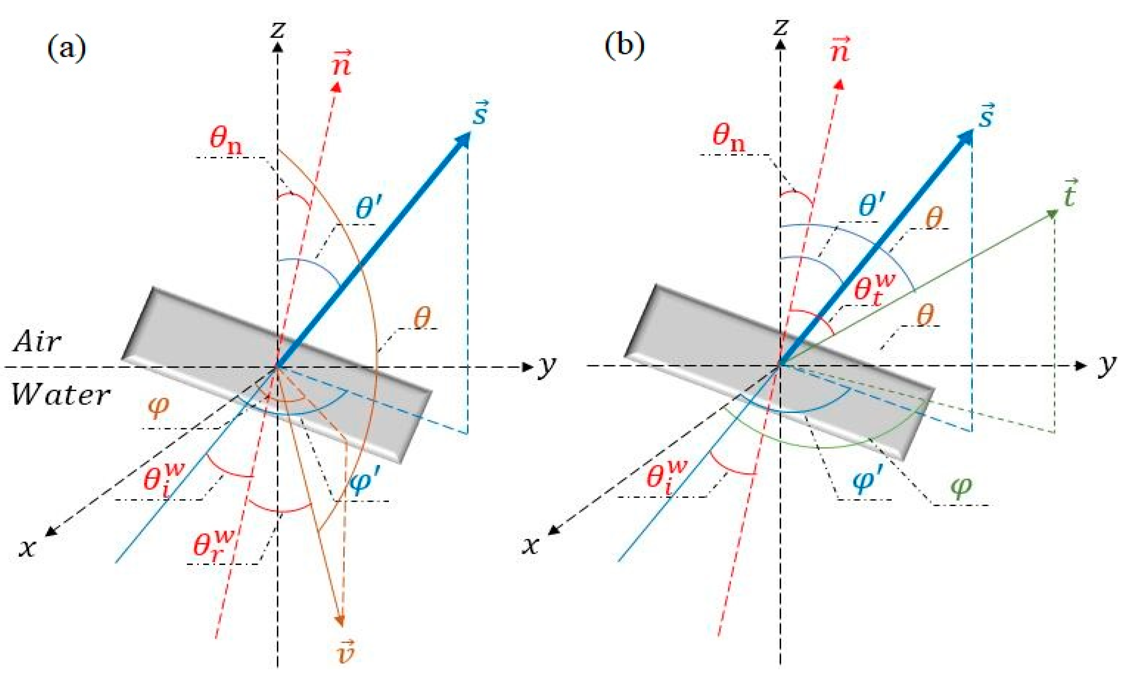
2.2. The Reflection Matrix of Wave Facets

The reflection matrix of wave facets $\mathit{r}$ describes a situation where incident light is reflected into direction $\left(\mu ,\phi \right)$ from direction $\left(\mu \prime , \phi \prime \right)$, where $\mu =cos\left(\mathsf{\theta }\right)$, $\mu \prime =\cos \left(\mathsf{\theta }\prime \right)$, $\mathsf{\theta }$ and $\mathsf{\theta }\prime$ are zenith angles measured from the positive z axis, and $\phi$ and $\phi \prime$ are azimuth angles measured from the positive x-axis in the anticlockwise direction when looking downward. $\mathit{r}$ is written as follows:

$$\mathit{r}\left({\mu }^{\prime },{\phi }^{\prime },\mu ,\phi \right)=S\left(\mu ,{\mu }^{\prime }\right)\frac{\pi p\left({\mu }_n,{\phi }_n\right)}{4\left|\mu \right|\left|{\mu }^{\prime }\right|{\mu }_n}\mathit{R}\left(\pi -{\chi }_2\right)\mathit{R}\mathit{F}\left({\theta }_i\right)\mathit{R}\left(-{\chi }_1\right),$$

(3)

where $p\left({\mu }_n,{\phi }_n\right)$ is given by Equation (1), and $S\left(\mu ,{\mu }^{\prime }\right)$ is the shadowing function accounting for the fact that the lidar light may be blocked by wave facet slopes [27,28]. $S\left(\mu ,{\mu }^{\prime }\right)$ is expressed as follows:

$$S\left(\mu ,{\mu }^{\prime }\right)=\frac{1}{1+\Lambda \left(\left|\mu \right|\right)+\Lambda \left(\left|\mu \prime \right|\right)},$$

(4)

where

$$\Lambda \left(\mu \right)=\frac{1}{2}\left\{\frac{1}{\sqrt{\pi }}\frac{1}{\eta }\exp \left(-{\eta }^2\right)-\mathrm{erfc}\left(\eta \right)\right\}.$$

(5)

$\eta$ is defined as

$$\eta =\frac{\mu }{\sigma \sqrt{1-{\mu }^2}}.$$

(6)

$\mathrm{erfc}$ is the complementary error function, and $\sigma$ is given by Equation (2).

$\mathit{R}\left(\chi \right)$ is the rotation matrix applied for the transition from the incident meridian plane to the reflection plane and from the reflection plane to the reflected meridian plane. It is expressed as follows:

$$\mathit{R}\left(\chi \right)=\left(\begin{array}{cccc}1& 0& 0& 0\\ 0& \cos 2\chi & \sin 2\chi & 0\\ 0& -\sin 2\chi & \cos 2\chi & 0\\ 0& 0& 0& 1\end{array}\right),$$

(7)

where ${\chi }_1$ and ${\chi }_2$ are the rotation angles shown in Figure 1.

For the air-incident case (see Figure 2a), the light is reflected toward the atmosphere onto the sea surface (reflection “air to air”). The surface reflection matrix $\mathit{raa}\left({\mu }^{\prime }, {\phi }^{\prime },\mu ,\phi \right)$ whose detailed calculation can be found in Appendix A is expressed as follows:

$$\mathit{raa}\left({\mu }^{\prime },{\phi }^{\prime },\mu ,\phi \right)=S\left(\mu ,{\mu }^{\prime }\right)\frac{\pi p\left({\mu }_n,{\phi }_n\right)}{4\left|\mu \right|\left|{\mu }^{\prime }\right|{\mu }_n}\mathit{R}\left(\pi -{\chi }_2\right)\mathit{R}{\mathit{F}}_{\mathit{A}\mathit{A}}\left({\theta }_i^a\right)\mathit{R}\left(-{\chi }_1\right).$$

(8)

The air-to-air Fresnel reflection matrix $\mathit{R}{\mathit{F}}_{\mathit{A}\mathit{A}}\left({\theta }_i^a\right)$ is a function of the incidence angle ${\theta }_i^a$ in the reflection plane and is expressed as follows:

$$\mathit{R}{\mathit{F}}_{\mathit{A}\mathit{A}}\left({\theta }_i^a\right)=\left(\begin{array}{c}\begin{array}{c}{r}_{11}^a\\ r_{12}^a\\ 0\end{array}\\ 0\end{array}\begin{array}{c}\begin{array}{c}{r}_{12}^a\\ r_{11}^a\\ 0\end{array}\\ 0\end{array}\begin{array}{c}\begin{array}{c}0\\ 0\\ r_{33}^a\end{array}\\ r_{34}\end{array}\begin{array}{c}\begin{array}{c}0\\ 0\\ r_{34}^a\end{array}\\ r_{33}\end{array}\right),$$

(9)

where

$$\{\begin{array}{c}{r}_{11}^a({\theta }_i^a)=0.5\times [{(r_l^a({\theta }_i^a))}^2+{(r_r^a({\theta }_i^a))}^2]\\ r_{11}^a({\theta }_i^a)=0.5\times [{(r_l^a({\theta }_i^a))}^2-{(r_r^a({\theta }_i^a))}^2]\\ r_{33}^a({\theta }_i^a)=Re(r_l^a({\theta }_i^a)\times r_r^{a*}({\theta }_i^a))\\ r_{34}^a({\theta }_i^a)=Im(r_l^a({\theta }_i^a)\times r_r^{a*}({\theta }_i^a))\end{array}$$

(10)

In Equation (10), $Re()$ and $Im()$ are the real and imaginary parts, respectively. The asterisk denotes the complex conjugate. $r_l^a\left({\theta }_i\right)$ and $r_r^a\left({\theta }_i\right)$ are the reflection coefficients of the parallel and vertical components of reflected light, respectively.

$$\{\begin{array}{c}{r}_l^a\left({\theta }_i^a\right)=\frac{m^{2}cos{\theta }_i^a-\sqrt{m^2-{sin}^2{\theta }_i^a}}{m^{2}cos{\theta }_i^a+\sqrt{m^2-{sin}^2{\theta }_i^a}}\\ r_r^a\left({\theta }_i^a\right)=\frac{cos{\theta }_i^a-\sqrt{m^2-{sin}^2{\theta }_i^a}}{cos{\theta }_i^a+\sqrt{m^2-{sin}^2{\theta }_i^a}}\end{array},$$

(11)

where m is the water refractive index. ${\theta }_i^a$ can be calculated using the formulas in the Appendix A.

For the water-incident case (see Figure 3a), the light is reflected toward the water onto the under-side of the sea surface (reflection “sea to sea”). Its surface reflection matrix $\mathit{r}\mathit{w}\mathit{w}\left({\mu }^{\prime }, {\phi }^{\prime },\mu ,\phi \right)$ is expressed as follows:

$$\mathit{r}\mathit{w}\mathit{w}\left({\mu }^{\prime },{\phi }^{\prime },\mu ,\phi \right)=S\left(\mu ,{\mu }^{\prime }\right)\frac{\pi p\left({\mu }_n,{\phi }_n\right)}{4\left|\mu \right|\left|{\mu }^{\prime }\right|{\mu }_n}\mathit{R}\left(\pi -{\chi }_2\right)\mathit{R}{\mathit{F}}_{\mathit{W}\mathit{W}}\left({\theta }_i^w\right)\mathit{R}\left(-{\chi }_1\right).$$

(12)

The water–water Fresnel reflection matrix $\mathit{R}{\mathit{F}}_{\mathit{W}\mathit{W}}\left({\theta }_i^w\right)$ is a function of the incidence angle ${\theta }_i^w$ in the reflection plane. $\mathit{R}{\mathit{F}}_{\mathit{W}\mathit{W}}\left({\theta }_i^w\right)$ is expressed in the same way as Equations (10) and (11), but $r_l^w\left({\theta }_i^w\right)$ and $r_r^w\left({\theta }_i^w\right)$ are different from $r_l^a\left({\theta }_i^a\right)$ and $r_r^a\left({\theta }_i^a\right)$.

$$\{\begin{array}{c}{r}_l^w\left({\theta }_i^w\right)=\frac{cos{\theta }_i^w-m\sqrt{1-m^2{sin}^2{\theta }_i^w}}{cos{\theta }_i^w+m\sqrt{1-m^2{sin}^2{\theta }_i^w}}\\ r_r^w\left({\theta }_i^w\right)=\frac{mcos{\theta }_i^w-\sqrt{1-m^2{sin}^2{\theta }_i^w}}{cos{\theta }_i^w+\sqrt{1-m^2{sin}^2{\theta }_i^w}}\end{array}.$$

(13)

Note that the total reflection happens beyond the critical angle in water (${\theta }_{lim}=\arcsin \left(1/m\right)$); thus, one has

$$\{\begin{array}{c}{r}_{11}^w\left({\theta }_i^w>{\theta }_{lim}\right)=1\\ r_{12}^w\left({\theta }_i^w>{\theta }_{lim}\right)=0\\ r_{33}^w\left({\theta }_i^w>{\theta }_{lim}\right)=1\\ r_{34}^w\left({\theta }_i^w>{\theta }_{lim}\right)=0\end{array}.$$

(14)

2.3. The Transmission Matrix of Wave Facets

The transmission matrix of wave facets $\mathit{t}$ is used in the situation where an incident light is transmitted into direction $\left(\mu ,\phi \right)$ from direction $\left(\mu ’, \phi ’\right)$. $\mathit{t}$ is written as follows:

$$\mathit{t}\left({\mu }^{\prime },{\phi }^{\prime },\mu ,\phi \right)=S\left(\mu ,{\mu }^{\prime }\right)\frac{\pi p\left({\mu }_n,{\phi }_n\right)}{4\left|\mu \right|\left|{\mu }^{\prime }\right|{\mu }_n}\mathit{R}\left(\pi -{\chi }_2\right)\mathit{T}\mathit{F}\left({\theta }_i\right)\mathit{R}\left(-{\chi }_1\right)\times \frac{n_t^{2}cos{\theta }_{t}cos{\theta }_i}{{\left(n_{t}cos{\theta }_t-n_{i}cos{\theta }_i\right)}^2},$$

(15)

where $S\left(\mu ,{\mu }^{\prime }\right)$ is the shadowing function expressed in the same way as Equation (23). $n_i$ and $n_t$ are refractive indices of the incident and transmitted media, respectively. $\mathit{T}\mathit{F}\left({\theta }_i\right)$ is the Fresnel transmission matrix.

For the air-incident case (Figure 2b), the light is refracted into the sea from the atmosphere medium (“air–sea”). The transmission matrix $\mathit{taw}\left({\mu }^{\prime }, {\phi }^{\prime },\mu ,\phi \right)$ is expressed as follows:

$$\mathit{taw}\left({\mathit{\mu }}^{\prime },{\mathit{\phi }}^{\prime },\mathit{\mu },\mathit{\phi }\right)=\mathit{S}\left(\mathit{\mu },{\mathit{\mu }}^{\prime }\right)\frac{\mathit{\pi }\mathit{p}\left({\mathit{\mu }}_{\mathit{n}},{\mathit{\phi }}_{\mathit{n}}\right)}{4\left|\mathit{\mu }\right|\left|{\mathit{\mu }}^{\prime }\right|{\mathit{\mu }}_{\mathit{n}}}\mathit{R}\left(\mathit{\pi }-{\mathit{\chi }}_2\right)\mathit{T}{\mathit{F}}_{\mathit{A}\mathit{W}}\left({\mathit{\theta }}_{\mathit{i}}^{\mathit{a}}\right)\mathit{R}\left(-{\mathit{\chi }}_1\right)\times \frac{{\mathit{m}}^2\mathbf{cos}{\mathit{\theta }}_{\mathit{t}}^{\mathit{a}}\mathbf{cos}{\mathit{\theta }}_{\mathit{i}}^{\mathit{a}}}{{\left(\mathit{m}\mathbf{cos}{\mathit{\theta }}_{\mathit{t}}^{\mathit{a}}-\mathbf{cos}{\mathit{\theta }}_{\mathit{i}}^{\mathit{a}}\right)}^2}.$$

(16)

The air-to-sea Fresnel transmission matrix $\mathit{T}{\mathit{F}}_{\mathit{A}\mathit{W}}\left({\mathit{\theta }}_{\mathit{i}}^{\mathit{a}}\right)$ is expressed as follows:

$$\mathit{T}{\mathit{F}}_{\mathit{A}\mathit{W}}\left({\theta }_i^a\right)=\frac{mcos{\theta }_t^a}{cos{\theta }_t^a}\left(\begin{array}{c}\begin{array}{c}{t}_{11}^a\\ t_{12}^a\\ 0\end{array}\\ 0\end{array}\begin{array}{c}\begin{array}{c}{t}_{12}^a\\ t_{11}^a\\ 0\end{array}\\ 0\end{array}\begin{array}{c}\begin{array}{c}0\\ 0\\ t_{33}^a\end{array}\\ t_{34}^a\end{array}\begin{array}{c}\begin{array}{c}0\\ 0\\ t_{34}^a\end{array}\\ t_{33}^a\end{array}\right),$$

(17)

where

$$\{\begin{array}{c}{t}_{11}^a({\theta }_i^a)=0.5\times [{(t_l^a({\theta }_i^a))}^2+{(t_r^a({\theta }_i^a))}^2]\\ t_{11}^a({\theta }_i^a)=0.5\times [{(t_l^a({\theta }_i^a))}^2-{(t_r^a({\theta }_i^a))}^2]\\ t_{33}^a({\theta }_i^a)=Re(t_l^a({\theta }_i^a)\times t_r^{a*}({\theta }_i^a))\\ t_{34}^a({\theta }_i^a)=Im(t_l^a({\theta }_i^a)\times t_r^{a*}({\theta }_i^a))\end{array}$$

(18)

In Equation (18), $t_l^a\left({\theta }_i^a\right)$ and $t_r^a\left({\theta }_i^a\right)$ are the transmission coefficients of the parallel and vertical components of transmitted light, respectively.

$$\{\begin{array}{c}{t}_l^a\left({\theta }_i^a\right)=\frac{2mcos{\theta }_i^a}{m^{2}cos{\theta }_i^a+\sqrt{m^2-{sin}^2{\theta }_i^a}}\\ t_r^a\left({\theta }_i^a\right)=\frac{2cos{\theta }_i^a}{cos{\theta }_i^a+\sqrt{m^2-{sin}^2{\theta }_i^a}}\end{array}.$$

(19)

For the water-incident case (Figure 3b), the light is refracted into the atmosphere from the sea medium (“sea–air”). The transmission matrix $\mathit{twa}\left({\mu }^{\prime }, {\phi }^{\prime },\mu ,\phi \right)$ is expressed as follows:

$$\mathit{twa}\left({\mu }^{\prime },{\phi }^{\prime },\mu ,\phi \right)=S\left(\mu ,{\mu }^{\prime }\right)\frac{\pi p\left({\mu }_n,{\phi }_n\right)}{4\left|\mu \right|\left|{\mu }^{\prime }\right|{\mu }_n}\mathit{R}\left(\pi -{\chi }_2\right)\mathit{T}{\mathit{F}}_{\mathit{W}\mathit{A}}\left({\theta }_i^w\right)\mathit{R}\left(-{\chi }_1\right)\times \frac{cos{\theta }_t^{w}cos{\theta }_i^w}{{\left(mcos{\theta }_i^w-cos{\theta }_t^w\right)}^2}.$$

(20)

The sea-to-air Fresnel transmission matrix $\mathit{T}{\mathit{F}}_{\mathit{W}\mathit{A}}\left({\theta }_i^w\right)$ is expressed as follows:

$$\mathit{T}{\mathit{F}}_{\mathit{W}\mathit{A}}\left({\theta }_w^i\right)=\frac{\cos {\theta }_w^t}{m\cos {\theta }_w^i}\times \left(\begin{array}{c}\begin{array}{c}{t}_{11}^a\\ t_{12}^a\\ 0\end{array}\\ 0\end{array}\begin{array}{c}\begin{array}{c}{t}_{12}^a\\ t_{11}^a\\ 0\end{array}\\ 0\end{array}\begin{array}{c}\begin{array}{c}0\\ 0\\ t_{33}^a\end{array}\\ t_{34}^a\end{array}\begin{array}{c}\begin{array}{c}0\\ 0\\ t_{34}^a\end{array}\\ t_{33}^a\end{array}\right),$$

(21)

$t_{11}^w, t_{12}^w, t_{33}^w,$ and $t_{34}^w$ are expressed in the same way as in Equation (18), but $t_l^w\left({\theta }_i^w\right)$ and have some differences.

$$\{\begin{array}{c}{t}_l^w\left({\theta }_i^w\right)=\frac{2mcos{\theta }_i^w}{cos{\theta }_i^w+m\sqrt{1-m^2{sin}^2{\theta }_i^w}}\\ t_r^w\left({\theta }_i^w\right)=\frac{2mcos{\theta }_i^w}{cos{\theta }_i^w+\sqrt{1-m^2{sin}^2{\theta }_i^w}}\end{array}.$$

(22)

Beyond the critical angle ${\theta }_{lim}$, we have

$$\{\begin{array}{c}{t}_{11}^w\left({\theta }_i^w>{\theta }_{lim}\right)=0\\ t_{12}^w\left({\theta }_i^w>{\theta }_{lim}\right)=0\\ t_{33}^w\left({\theta }_i^w>{\theta }_{lim}\right)=0\\ t_{34}^w\left({\theta }_i^w>{\theta }_{lim}\right)=0\end{array}.$$

(23)

2.4. The Integration of Raa, Rww, Taw, and Twa

Using Equations (8), (12), (16), and (20), the reflection and transmission matrices of a small wave facet were calculated. Then, the Muller matrix within a certain viewing angle was obtained by integrating the zenith and azimuth angles as follows:

$$r_a\left({\mu }^{\prime },{\mu }_1,{\phi }_1,{\mu }_2,{\phi }_2\right)=\frac{1}{\pi }{{\displaystyle \int }}_{{\mu }_1}^{{\mu }_2}\mu d\mu {{\displaystyle \int }}_{{\phi }_1}^{{\phi }_2}d\phi \mathit{raa}\left({\mu }^{\prime },{\phi }^{\prime },\mu ,\phi \right) 0\le {\mu }_1<{\mu }_2\le 1;0\le {\phi }_1<{\phi }_2\le 2\pi .$$

(24)

$$t_a\left({\mu }^{\prime },{\mu }_1,{\phi }_1,{\mu }_2,{\phi }_2\right)=\frac{1}{\pi }{{\displaystyle \int }}_{{\mu }_1}^{{\mu }_2}\left|\mu \right|d\mu {{\displaystyle \int }}_{{\phi }_1}^{{\phi }_2}d\phi \mathit{taw}\left({\mu }^{\prime },{\phi }^{\prime },\mu ,\phi \right)-1\le {\mu }_1<{\mu }_2\le 0;0\le {\phi }_1<{\phi }_2\le 2\pi .$$

(25)

$$r_{\mathit{w}}\left({\mu }^{\prime },{\mu }_1,{\phi }_1,{\mu }_2,{\phi }_2\right)=\frac{1}{\pi }{{\displaystyle \int }}_{{\mu }_1}^{{\mu }_2}\left|\mu \right|d\mu {{\displaystyle \int }}_{{\phi }_1}^{{\phi }_2}d\phi \mathit{rww}\left({\mu }^{\prime },{\phi }^{\prime },\mu ,\phi \right) -1\le {\mu }_1<{\mu }_2\le 0;0\le {\phi }_1<{\phi }_2\le 2\pi .$$

(26)

$$t_w\left({\mu }^{\prime },{\mu }_1,{\phi }_1,{\mu }_2,{\phi }_2\right)=\frac{1}{\pi }{{\displaystyle \int }}_{{\mu }_1}^{{\mu }_2}\mu d\mu {{\displaystyle \int }}_{{\phi }_1}^{{\phi }_2}d\phi \mathit{twa}\left({\mu }^{\prime },{\phi }^{\prime },\mu ,\phi \right) 0\le {\mu }_1<{\mu }_2\le 1;0\le {\phi }_1<{\phi }_2\le 2\pi .$$

(27)

The Gaussian quadrature formulas were used for the integration. After that, we have

$${\mathit{S}}_{\mathit{r}\mathit{a}}={\mathit{r}}_{\mathit{a}}\ast {\mathit{S}}_{\mathbf{0}},$$

(28)

$${\mathit{S}}_{\mathit{t}\mathit{a}}={\mathit{t}}_{\mathit{a}}\ast {\mathit{S}}_{\mathbf{0}},$$

(29)

$${\mathit{S}}_{\mathit{r}\mathit{w}}={\mathit{r}}_{\mathit{w}}\ast {\mathit{S}}_{\mathbf{0}},$$

(30)

$${\mathit{S}}_{\mathit{t}\mathit{w}}={\mathit{t}}_{\mathit{w}}\ast {\mathit{S}}_{\mathbf{0}},$$

(31)

where ${\mathit{S}}_{\mathbf{0}}$ denotes the incident light of lidar. ${\mathit{S}}_{\mathit{r}\mathit{a}}$ and ${\mathit{S}}_{\mathit{t}\mathit{a}}$ are respectively reflected and transmitted lights of the air-incident case. Accordingly, ${\mathit{S}}_{\mathit{r}\mathit{w}}$ and ${\mathit{S}}_{\mathit{t}\mathit{w}}$ are respectively reflected and transmitted lights of the water-incident case.

2.5. Polarization and Depolarization of Reflection and Transmission

We used degree of total polarization (DoP) to quantify the polarization properties of reflection and transmission. DoP is defined as follows:

$$DoP= \frac{\sqrt{{\mathrm{Q}}^2+{\mathrm{U}}^2+{\mathrm{V}}^2}}{\mathrm{I}}.$$

(32)

In order to quantify the depolarization effects caused by the sea surface, the depolarization ratio ($\mathsf{\delta }$) was calculated as follows:

$$\mathsf{\delta }=\frac{I_r}{I_l}=\frac{\mathrm{I}-\mathrm{Q}}{\mathrm{I}+\mathrm{Q}}.$$

(33)

For the polarized lidar incident light, $\mathsf{\delta }$ is zero, which means that the vertical component is negligible. After the light propagates through the sea surface, the vertical component arises due to scattering. In general, $\mathsf{\delta }$ is less than 1. A value of $\mathsf{\delta }$ equal to 1 indicates that the polarized light was totally unpolarized. However, $\mathsf{\delta }$ is greater than 1 in some cases where parallel-polarized light becomes partially vertically polarized.

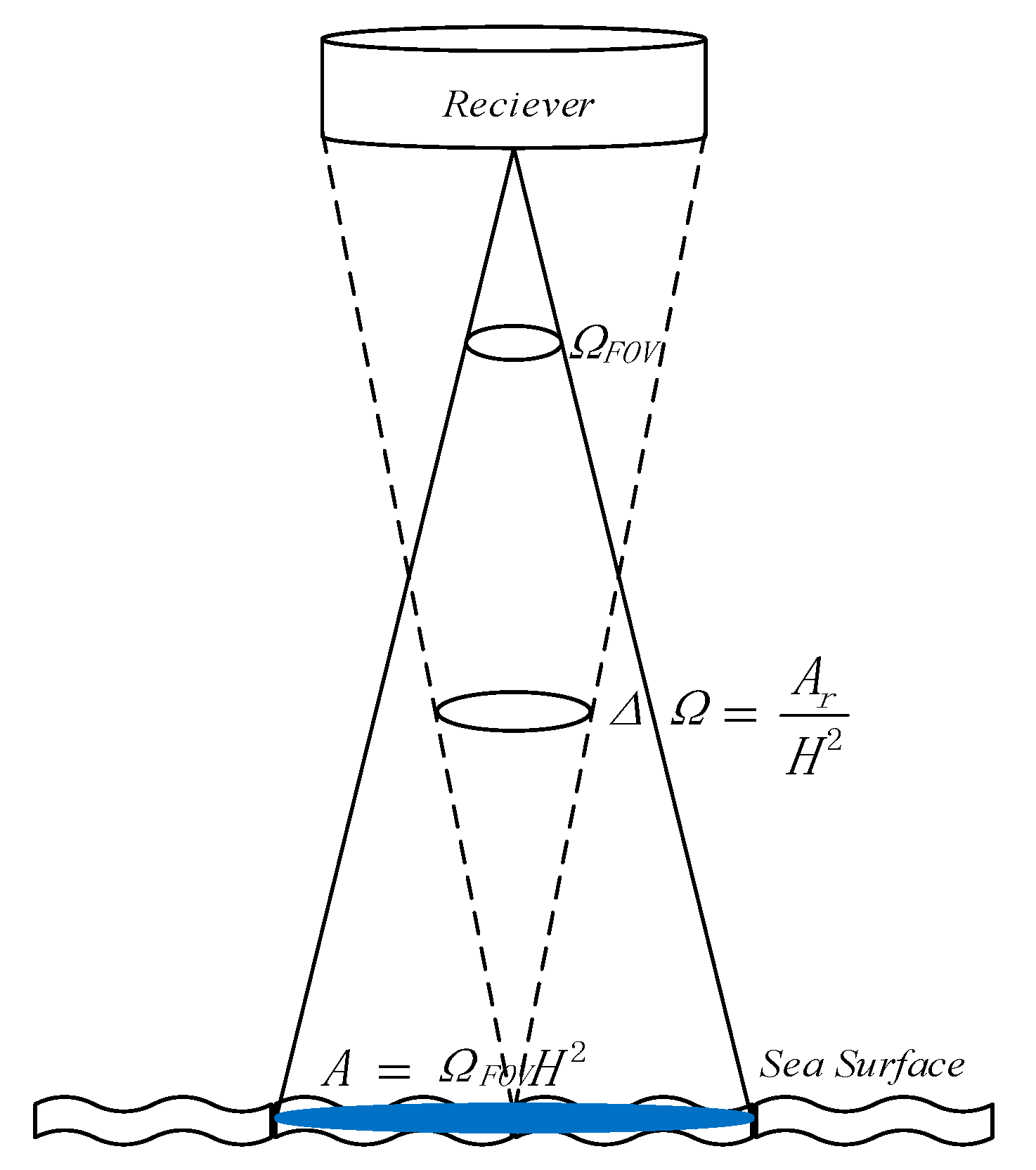
2.6. Simulation Model Coupled with Lidar System

An improved semi-analytic simulation model was developed for estimating the probability of photon scatter back to a remote receiver $E\left(k\right)$ at the surface coupled with lidar system parameters (see Figure 4).

$$E\left(k\right)=\frac{P\left(\mathsf{\Theta }\right)}{4\pi }\mathsf{\Delta }\mathsf{\Omega }\exp \left(\tau \right)=\frac{P\left(\theta \right)}{4\pi }\frac{A_r}{H^2}\exp \left(\tau \right),$$

(34)

where $P\left(\mathsf{\Theta }\right)$ is the scattering phase function value at angle $\mathsf{\Theta }$, $\mathsf{\Delta }\mathsf{\Omega }$ is the small solid received angle by a remote detector, $A_r$ is detector aperture, $H$ is lidar flight height, and $\tau$ is the atmosphere optical thickness. The solid angle of collision photon received by a remote detector is so small that the cosine value of the actual backscattering line is similar to the line perpendicular to the air/water interface. The atmosphere is purely Rayleigh atmosphere with no aerosols, and the oceanic constituents only consist of seawater molecules with no hydrosols. The factor of molecular depolarization in the air is zero. The detector height is 300 m, and the lidar frequency used here is 532 nm; thus, the atmosphere optical thickness can be negligible. The detector aperture $A_r$ is 0.06 m². The water absorption coefficient is 0.04 m⁻¹ and the scattering coefficient is 0.06 m⁻¹. To avoid the solar noise, we simplify the simulation and assume nighttime conditions (i.e., the lidar is the only light source).

The semi-analytic Monte Carlo radiative transfer model developed by Chen [12,14] is based on analytical estimate of the probability of photon scatter back to a remote receiver, and the lidar geometric model is considered for oceanographic lidar systems. The estimated value $E\left(k\right)$ of the fraction of photons collected by the remoter receiver upon a scattering event at collision point $k$ is calculated using Poole’s method [29].

As shown in Figure 4, whether the photon’s position is within the receiver field of view (FOV) needs to be determined.

$$x_k^2+y_k^2\le A,$$

(35)

$$A={\mathsf{\Omega }}_{FOV}{H}^2,$$

(36)

where ${\mathsf{\Omega }}_{FOV}$ is the receiver FOV solid angle, $A$ is the area at the surface seen by the receiver, and $x_k$ and ${\mathrm{y}}_k$ are the photon’s position in Cartesian coordinates.

3. Simulation Results

3.1. Model Validation

To validate our model, the results of unpolarized light (i.e., $S_0={\left[1,0,0,0\right]}^{\mathrm{T}}$) were compared with those of Nakajima [30]. Nakajima generalized a matrix method of solving the transfer of solar radiation in an atmosphere–ocean system with a wind-roughed ocean surface. He used an isotropic Gaussian distribution to assume the density function of the wave slope as in Equation (1), with ${\mathsf{\sigma }}^2=0.00534W$ in his model.

The unidirectional reflectivity was calculated using Equation (24a) where ${\mathsf{\mu }}_1=0,{\mathsf{\mu }}_2=1,{\mathsf{\phi }}_1=0,{\mathrm{and}\mathsf{\phi }}_2=2\mathsf{\pi }$ (i.e., the upper hemispherical integration), and Equation (24b) where ${\mathsf{\mu }}_1=-1,{\mathsf{\mu }}_2=0,{\mathsf{\phi }}_1=0,{\mathrm{and}\mathsf{\phi }}_2=2\mathsf{\pi }$ (i.e., the lower hemispherical integration).

Figure 5a compares the reflectivity in our model, shown as solid lines, with Nakajima’s outputs, which are highlighted with asterisks on dashed lines. The solid lines match the dashed lines well, which indicates an excellent agreement both in the air-incident case (light across the surface from air to sea) and in the water-incident case (light across the surface from sea to air). Figure 5b presents the absolute percentage deviation (APD) between the two models. A large difference happened when the wind speed was 0 m/s, which was due to the little difference between ${\sigma }^2$ and $W$ in the two models. In Nakajima’s model, ${\sigma }^2$ = 0 (i.e., a flat sea surface), when $W$ was 0. In our model, ${\sigma }^2\left(W=0\right)$ was 0.003. In reality, the sea surface is not flat, although there is no wind blowing, (i.e., ${\sigma }_{W=0}^2\ne 0$). Our model is consistent with a previous study [31], indicating that our model is more precise. The maximum value of APD occurs near the critical angle for total internal reflection, but in our model, a little upwelling energy still leaked through the surface into the air due to the roughness. As the wind speed increased, the APD between the two models narrowed rapidly. Figure 5c,d present the regression plots of outputs between the two models for air-incident and water-incident cases, respectively. It shows that the adjusted R-squared between them was nearly one. As shown in

Table 1. Statistics of the differences between our results and Nakajima’s results. AD—absolute difference; APD—absolute percentage deviation; MAD—mean absolute difference; MAPD—mean absolute percentage deviation;

	W (m/s)	R2	RMSE	MaxAD	MaxAPD	MAD	MAPD
Air-incident	0	0.9938	0.0491	0.2513	25.4646%	0.0143	2.3642%
	0.83	0.9998	0.0138	0.0599	8.4826%	0.0054	1.5342%
	3.33	1.0000	0.0044	0.0178	3.4032%	0.0020	0.8736%
	7.49	1.0000	0.0013	0.0049	1.2275%	0.0006	0.3722%
	15.29	1.0000	0.0002	0.0006	0.1988%	0.0001	0.0677%
Water-incident	0	0.9952	0.0489	0.2926	59.9937%	0.0188	5.0894%
	0.83	0.9995	0.0155	0.0543	25.1187%	0.0085	2.9464%
	3.33	0.9999	0.0059	0.0154	9.1151%	0.0041	1.5886%
	7.49	1.0000	0.0025	0.0062	3.0189%	0.0017	0.6922%
	15.29	1.0000	0.0005	0.0010	0.3833%	0.0003	0.1180%

, the root mean squared error (RMSE) between them was very small except at the zero speed.

Table 1 shows the statistics of the differences. AD means the absolute value of the difference. MAD and MAPD are the mean values of AD and APD, respectively. The table shows that the MADs between the two models were no more than 0.01, and the MAPDs were no more than 3% when the wind was larger than 0 m/s. Both statistics indicate that our model is accurate enough for simulating light propagation across a sea surface.

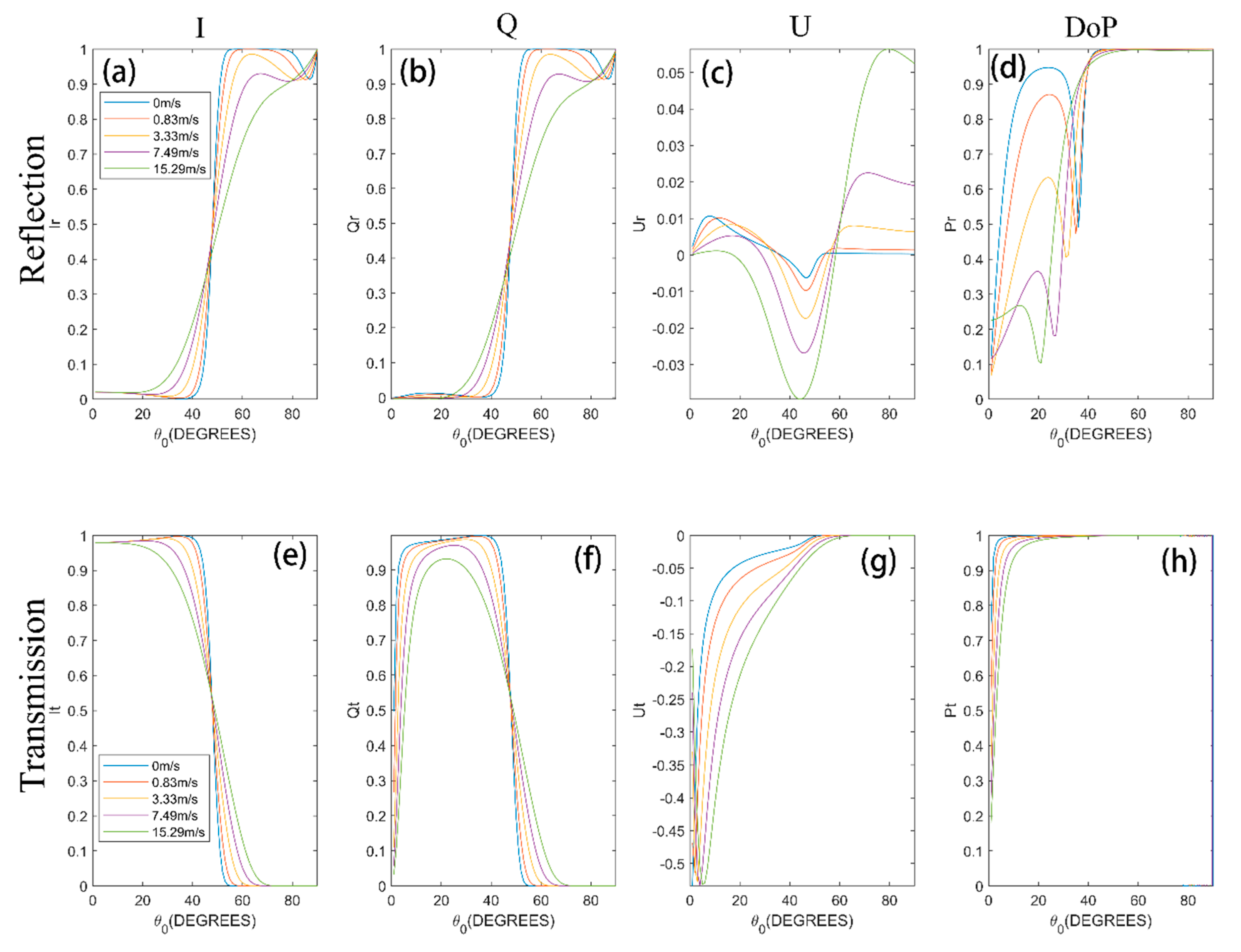
3.2. Sea Surface Reflection and Transmission of Lidar

Then, we applied our model for polarized lidar (i.e., $S_0={\left[1,1,0,0\right]}^{\mathrm{T}}$). Figure 6a–c present the Stokes parameters I, Q, and U of reflected light for the air-incident case, respectively. Figure 6e–g present the Stokes parameters of transmission light accordingly. Figure 6d,h present the DoP of reflected and transmitted light, respectively. Figure 7 shows the results of reflection and transmission of the ocean surface for the water-incident polarized lidar ($S_0={\left[1,1,0,0\right]}^{\mathrm{T}}$). Specifically, Figure 7a–c present the Stokes parameters I, Q, and U of reflected light for the water-incident case, respectively. Figure 7e–g present the Stokes parameters of transmission accordingly. Similarly, Figure 7d,h present the DoP of reflected light and transmission light of water-incident lidar, respectively. Compared with Figure 5a, Figure 6a shows that the reflectivity of polarized lidar was much lower than that of unpolarized light. In reality, the reflectivity varies with the polarization status of incident light. show the apparent depolarization of reflection. For the reflection of the air-incident case, the DoP reached the minimum value near $\theta =53°$, which is the Brewster angle. As the wind speed increased, the reflectivity decreased, while depolarization increased. With a proper incident angle near 53$°$ shown in Figure 6a, more energy would be transmitted into the water, which could expand the detective depth for oceanographic lidar.

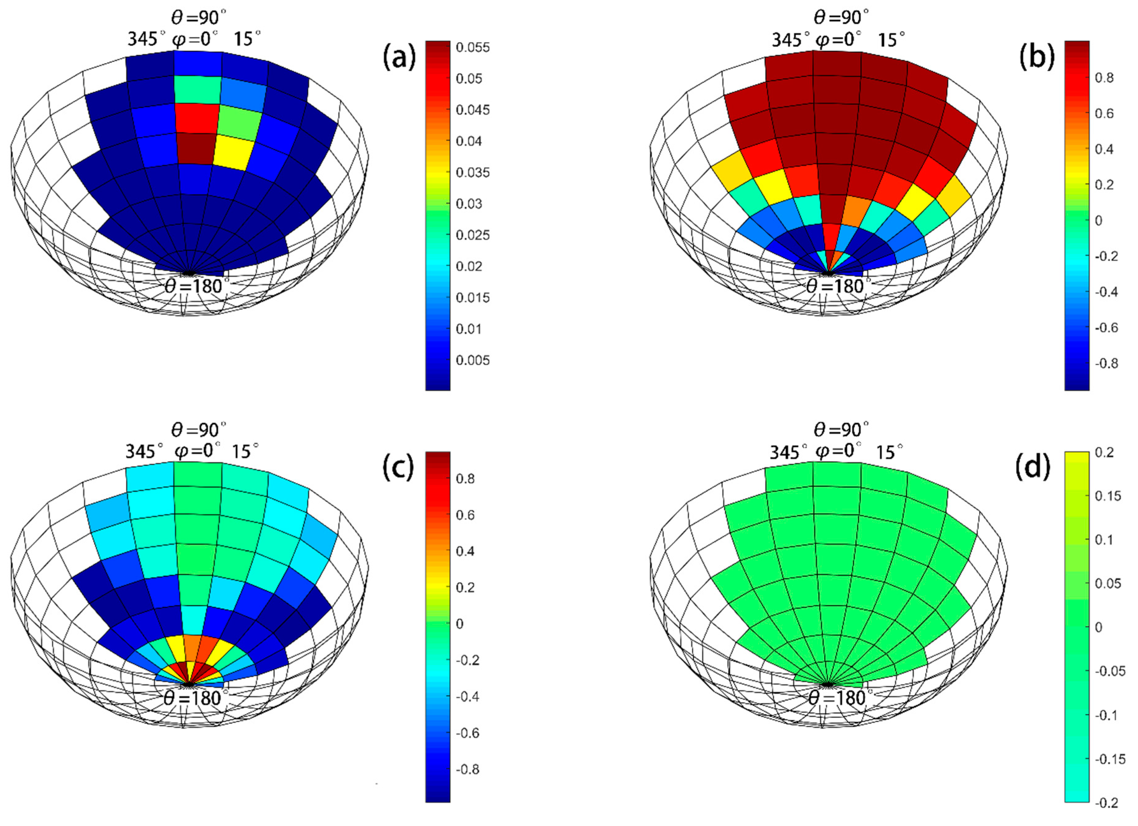
3.3. Air-Incident Reflection Pattern

The energy pattern in different azimuth and zenith angles of polarized lidar was analyzed. Figure 8a presents the percentage of the air-incident energy, which was reflected into each direction for quads of angular size $10°\times 15°$ in zenith and azimuthal angles when wind speed was 10 m/s. The incident light was completely polarized, i.e., $S_0={\left[1,1,0,0\right]}^{\mathrm{T}}$. The incident direction was 45° from the zenith (i.e., ${\theta }^{\prime }=135°$). Compared with unpolarized light whose reflectivity was 3.1%, only 0.7% of the air-incident energy was reflected, and the remaining 99.3% was transmitted into water. The maximum value was in the specular quad near $\theta =45°$. Figure 8b presents horizontal polarization (>0) and vertical polarization (<0). An evident depolarization is shown in Figure 8b. The 45° polarization shown in Figure 8c arose because of reflected light titled by wave facets. As shown in Figure 8d, the circular polarized light was nearly zero.

3.4. Air-Incident Transmission Pattern

Subsequently, the transmission energy was analyzed. Figure 9a shows the percentage of the air-incident energy, which was transmitted into the water across the sea surface. Figure 9b–d show the horizontal, 45°, and circular polarization, respectively. The wind-blown rough sea surface had less influence on the transmission light. The transmitted lights were concentrated on the specular-refracted quad near $\theta =32°$. The energy decreased sharply to zero when it was transmitted away from the specular-refracted quad. Figure 9b shows that the sea surface had less of an effect on depolarization for transmission light compared with reflected light. The 45° polarization shown in Figure 9c arose because of transmission light titled by wave facets. As shown in Figure 9d, the circular polarization was nearly zero.

3.5. Water-Incident Reflection Pattern

The pattern of water-incident lidar was plotted in the same way as that of air-incident lidar. Figure 10a presents the percentage of the water-incident energy, which was reflected into water onto the under-side of the sea surface. In the case of 45° incident and 10 m/s wind, the reflectivity was 34.51%, less than that of unpolarized light (38.08%). The energy was distributed around the specular reflectance quad near $\theta =45°$. Figure 10b presents the horizontal and vertical polarization. The reflected light was depolarized due to scattering. Figure 10c presents 45° polarization. The circular polarization, shown in Figure 10d, was almost zero.

3.6. Water-Incident Transmission Pattern

Figure 11a shows that the energy was concentrated on the specular-refracted quad near $\theta =70°$ for transmitted light. The energy decreased sharply to zero when it was transmitted away from the specular-refracted quad. Figure 11b presents the horizontal polarization. We find that depolarization was not as obvious as reflectance. The polarization degree of transmittance was above 0.995, while the polarization degree of reflectance was about 0.85, because it is difficult to change the polarization of the light refracted by the wave facets [19]. The 45° polarization, shown in Figure 11c, arose because transmittance was titled by wave facets. As shown in Figure 11d, the circular polarization was almost zero.

3.7. Depolarization of Reflection and Transmission

Depolarization ratio $\mathsf{\delta }$ is shown in Figure 12 for different incident zenith angles. The high DoP in Figure 6d,h and Figure 6d,h corresponded to a little $\mathsf{\delta }$ value. The $\mathsf{\delta }$ value near one was consistent with a low DoP. Figure 12a shows the depolarization ratio of reflection of air-incident light. The depolarization ratio was positively correlated with wind speed. The reflected light would become unpolarized with too high speed. In some cases, the $\mathsf{\delta }$ value beyond one indicated that parallel-polarized lidar was transformed into partially vertically polarized light. Only in certain conditions, where wind is gentle and incident angle is between 20$°$ to 40$°$ or beyond 60$°$, can the depolarization of reflected light be negligible. Figure 12b presents the depolarization ratio of transmission of air-incident light. When the wind speed was beyond 20$°$, the depolarization was nearly zero no matter how strong the wind was. The depolarization ratio of reflection for water-incident light had the same effects as air-incident light. The depolarized influence of transmission for water-incident light, shown in Figure 12d, was negligible with large zenith angles. We find an unusual depolarization phenomenon whereby polarized lidar light was severely depolarized when the zenith angle was small, even in the case of transmission. From this point, the depolarization effects of sea surface were not negligible. To minimize the effects of sea surfaces, it would be better if the incident angle of lidar was bigger than 20$°$ and less than 40$°$. Alternatively, if the depolarization rate of sea surfaces is calculated based on the geometry of lidar and wind speed, then the depolarization rate of the echo signal minus depolarization rate caused by the ocean–air interface could be regarded as the rectified depolarization rate of ocean constituents.

4. Discussion

In this study, we focused on the depolarization of the sea surface. Before applying this model for polarized lidar, unpolarized solar light was used to validate it. Another important verification involved checking the energy conservation. In Nakajima’s model, a normalized modification of the reflection and transmission was employed based on energy deficiency, which reached about 10% for large angles of incidence. This energy deficiency was explained as a result of multiple scattering between wave facets [20,30]. However, some radiative transfer codes generally do not take this problem into consideration [20,32,33]. In this work, we avoided normalizing Equations (3) and (15) to simplify the calculation. The effects of energy deficiency on depolarization will be further analyzed in future work.

Considering the depolarization of sea surface and dynamic range of the receiver, a moderate incident angle between 20$°$ and 40$°$ would be better to minimize the effects of the air–sea interface for shipboard oceanographic lidar. With a large incident angle, the receiver would be saturated by the energy reflected from the sea surface, which would mask the signal from under the sea surface. Future studies will account for more realistic elements such as different ocean constituents and diffuse solar radiation to calculate an optimal geometry.

Based on the relationship between the signal echoed from the sea surface and the wave slope and wind speed, the lidar shows potential in detecting sea wave and wind. Combined with the geometry of lidar, depolarization effects of the sea surface could be accounted for from the echo signal; thus, the retrieval for properties of ocean constituents can be effectively improved, with higher accuracy.

5. Conclusions

In this study, we developed an improved model to calculate the depolarization ratio of reflection and transmission for polarization lidar propagating through a rough sea surface based on the Cox–Munk surface model and Gaussian quadrature method. The comparison of different simulations indicated that our method is effective for simulating the propagation of lidar interacting with a wind-blown rough sea–air interface. The shadowing effects were also considered in this model. In particular, we analyzed the polarized properties in different azimuth and zenith angles and found that rough sea surfaces have a non-negligible influence on polarization of incident light. For unpolarized light, the reflectance tends to polarize the source light; however, for lidar light, it depolarizes the source light. The depolarization of the sea surface is not negligible at small zenith angles. Our model will be applied to simulate the echo signal of oceanographic lidar in future work, and the simulation results will also be used to retrieve the depolarization within water. In addition, a comparison between measurements and simulations will be carried out to improve our method.

References

1. Churnside, J.H.; Marchbanks, R.D. Subsurface plankton layers in the Arctic Ocean. Geophys. Res. Lett. 2015, 42, 4896–4902. [Google Scholar] [CrossRef]
2. Churnside, J.H.; Donaghay, P.L. Thin scattering layers observed by airborne lidar. ICES J. Mar. Sci. J. Cons. 2009, 66, 778–789. [Google Scholar] [CrossRef]
3. Liu, H.; Chen, P.; Mao, Z.; Pan, D.; He, Y. Subsurface plankton layers observed from airborne lidar in Sanya Bay, South China Sea. Opt. Express 2018, 26, 29134–29147. [Google Scholar] [CrossRef]
4. Chen, P.; Pan, D. Ocean Optical Profiling in South China Sea Using Airborne LiDAR. Remote Sens. 2019, 11, 1826. [Google Scholar] [CrossRef] [Green Version]
5. Churnside, J.H.; Marchbanks, R.D. Inversion of oceanographic profiling lidars by a perturbation to a linear regression. Appl. Opt. 2017, 56, 5228–5233. [Google Scholar] [CrossRef] [PubMed]
6. Churnside, J.; Hair, J.; Hostetler, C.; Scarino, A. Ocean Backscatter Profiling Using High-Spectral-Resolution Lidar and a Perturbation Retrieval. Remote Sens. 2018, 10, 2003. [Google Scholar] [CrossRef] [Green Version]
7. Chen, P.; Pan, D.; Mao, Z.; Liu, H. A Feasible Calibration Method for Type 1 Open Ocean Water LiDAR Data Based on Bio-Optical Models. Remote Sens. 2019, 11, 172. [Google Scholar] [CrossRef] [Green Version]
8. Saylam, K.; Brown, R.A.; Hupp, J.R. Assessment of depth and turbidity with airborne Lidar bathymetry and multiband satellite imagery in shallow water bodies of the Alaskan North Slope. Int. J. Appl. Earth Obs. Geoinf. 2017, 58, 191–200. [Google Scholar] [CrossRef]
9. Richter, K.; Maas, H.-G.; Westfeld, P.; Weiß, R. An Approach to Determining Turbidity and Correcting for Signal Attenuation in Airborne Lidar Bathymetry. PFG—J. Photogramm. Remote Sens. Geoinf. Sci. 2017, 85, 31–40. [Google Scholar] [CrossRef]
10. Churnside, J.H. Polarization effects on oceanographic lidar. Opt Express 2008, 16, 1196–1207. [Google Scholar] [CrossRef]
11. Hostetler, C.A.; Behrenfeld, M.J.; Hu, Y.; Hair, J.W.; Schulien, J.A. Spaceborne Lidar in the Study of Marine Systems. Annu. Rev. Mar. Sci. 2018, 10, 121–147. [Google Scholar] [CrossRef] [PubMed] [Green Version]
12. Chen, P.; Pan, D.; Mao, Z.; Liu, H. Semi-Analytic Monte Carlo Model for Oceanographic Lidar Systems: Lookup Table Method Used for Randomly Choosing Scattering Angles. Appl. Sci. 2018, 9, 48. [Google Scholar] [CrossRef] [Green Version]
13. Otsuki, S. Multiple scattering of polarized light in turbid infinite planes: Monte Carlo simulations. J. Opt. Soc. Am. A Opt. Image Sci. Vis. 2016, 33, 988–996. [Google Scholar] [CrossRef]
14. Chen, P.; Pan, D.; Mao, Z.; Liu, H. Semi-analytic Monte Carlo radiative transfer model of laser propagation in inhomogeneous sea water within subsurface plankton layer. Opt. Laser Technol. 2019, 111, 1–5. [Google Scholar] [CrossRef]
15. Abdallah, H.; Bailly, J.S.; Baghdadi, N.N.; Saint-Geours, N.; Fabre, F. Potential of Space-Borne LiDAR Sensors for Global Bathymetry in Coastal and Inland Waters. IEEE J. Sel. Top. Appl. Earth Obs. Remote Sens. 2013, 6, 202–216. [Google Scholar] [CrossRef] [Green Version]
16. Abdallah, H.; Baghdadi, N.; Bailly, J.-S.; Pastol, Y.; Fabre, F. Wa-LiD: A new LiDAR simulator for waters. Geosci. Remote Sens. Lett. IEEE 2012, 9, 744–748. [Google Scholar] [CrossRef] [Green Version]
17. Jamet, C.; Ibrahim, A.; Ahmad, Z.; Angelini, F.; Babin, M.; Behrenfeld, M.J.; Boss, E.; Cairns, B.; Churnside, J.; Chowdhary, J.; et al. Going Beyond Standard Ocean Color Observations: Lidar and Polarimetry. Front. Mar. Sci. 2019, 6. [Google Scholar] [CrossRef]
18. Chami, M.; Lafrance, B.; Fougnie, B.; Chowdhary, J.; Harmel, T.; Waquet, F. OSOAA: A vector radiative transfer model of coupled atmosphere-ocean system for a rough sea surface application to the estimates of the directional variations of the water leaving reflectance to better process multi-angular satellite sensors data over the ocean. Opt Express 2015, 23, 27829–27852. [Google Scholar] [CrossRef] [Green Version]
19. Mobley, C.D. Polarized reflectance and transmittance properties of windblown sea surfaces. Appl. Opt. 2015, 54, 4828–4849. [Google Scholar] [CrossRef]
20. Zhai, P.-W.; Hu, Y.; Chowdhary, J.; Trepte, C.R.; Lucker, P.L.; Josset, D.B. A vector radiative transfer model for coupled atmosphere and ocean systems with a rough interface. J. Quant. Spectrosc. Radiat. Transf. 2010, 111, 1025–1040. [Google Scholar] [CrossRef]
21. Rozanov, V.V.; Dinter, T.; Rozanov, A.V.; Wolanin, A.; Bracher, A.; Burrows, J.P. Radiative transfer modeling through terrestrial atmosphere and ocean accounting for inelastic processes: Software package SCIATRAN. J. Quant. Spectrosc. Radiat. Transf. 2017, 194, 65–85. [Google Scholar] [CrossRef] [Green Version]
22. Deuzé, J.L.; Herman, M.; Santer, R. Fourier series expansion of the transfer equation in the atmosphere-ocean system. J. Quant. Spectrosc. Radiat. Transf. 1989, 41, 483–494. [Google Scholar] [CrossRef]
23. Hieronymi, M. Polarized reflectance and transmittance distribution functions of the ocean surface. Opt Express 2016, 24, A1045–A1068. [Google Scholar] [CrossRef] [PubMed]
24. D’Alimonte, D.; Kajiyama, T. Effects of light polarization and waves slope statistics on the reflectance factor of the sea surface. Opt Express 2016, 24, 7922–7942. [Google Scholar] [CrossRef] [Green Version]
25. Cox, C.; Munk, W. Statistics of the sea surface derived from Sun glitter. J. Mar. Res. 1954, 13, 198–227. [Google Scholar]
26. Cox, C.; Munk, W. Measurement of the Roughness of the Sea Surface from Photographs of the Sun’s Glitter. J. Opt. Soc. Am. 1954, 44. [Google Scholar] [CrossRef]
27. Sancer, M. Shadow-corrected electromagnetic scattering from a randomly rough surface. IEEE Trans. Antennas Propag. 1969, 17, 577–585. [Google Scholar] [CrossRef]
28. Smith, B. Geometrical shadowing of a random rough surface. IEEE Trans. Antennas Propag. 1967, 15, 668–671. [Google Scholar] [CrossRef]
29. Poole, L.R.; Venable, D.D.; Campbell, J.W. Semianalytic Monte Carlo radiative transfer model for oceanographic lidar systems. Appl. Opt. 1981, 20, 3653–3656. [Google Scholar] [CrossRef]
30. Nakajima, T.; Tanaka, M. Effect of wind-generated waves on the transfer of solar radiation in the atmosphere-ocean system. J. Quant. Spectrosc. Radiat. Transf. 1983, 29, 521–537. [Google Scholar] [CrossRef]
31. Ebuchi, N.; Kizu, S. Probability distribution of surface wave slope derived using Sun glitter images from geostationary meteorological satellite and surface vector winds from scatterometers. J. Oceanogr. 2002, 58, 477–486. [Google Scholar] [CrossRef]
32. Lenoble, J.; Herman, M.; Deuzé, J.L.; Lafrance, B.; Santer, R.; Tanré, D. A successive order of scattering code for solving the vector equation of transfer in the earth’s atmosphere with aerosols. J. Quant. Spectrosc. Radiat. Transf. 2007, 107, 479–507. [Google Scholar] [CrossRef]
33. Mishchenko, M.I.; Travis, L.D. Satellite retrieval of aerosol properties over the ocean using polarization as well as intensity of reflected sunlight. J. Geophys. Res. Atmos. 1997, 102, 16989–17013. [Google Scholar] [CrossRef] [Green Version]
Figure 1. Relationship between the scattering and reflection matrices: s ,   v are the unit vectors of the incident and reflected light respectively; χ 1 is the rotation angle between the incident meridian plane and the reflection plane; χ 2 is the rotation angle between the reflection plane and the reflection meridian plane.
Applsci 10 01030 g001
Figure 2. Geometry of the propagation of the lidar light across a rough sea surface for the air-incident case. (a) Reflection “air to air”. (b) Refraction “air to sea”. The notations are as follows: θ i a ,   θ r a ,   and   θ t a are respectively the incidence angle, reflection angle, and refraction angle relative to the wave facet normal vector n in the scattering plane. s ,   v ,   and   t are the unit vectors of the incident, reflected, and transmitted light, respectively. θ is the zenith angle of the incident light, θ is the zenith angle of the exit light (reflected light for the reflection matrix and transmitted light for the transmission matrix), and φ is the azimuth angle.
Applsci 10 01030 g002
Figure 3. Geometry of the propagation of the lidar light across a rough sea surface for the water-incident case. (a) Reflection “sea to sea”. (b) Refraction “sea to air”. All notations are as follows: θ i w ,   θ r w ,   and   θ t w are respectively the incidence angle, reflection angle, and refraction angle relative to the wave facet normal vector n in the scattering plane; s ,   v ,   and   t are the unit vectors of the incident, reflected, and transmitted light respectively; θ is the zenith angle of the incident light, θ is the zenith angle of the exit light (reflected light for the reflection matrix and transmitted light for the transmission matrix), and φ is the azimuth angle.
Applsci 10 01030 g003
Figure 4. Lidar geometric model for analytically estimating the probability of photon scatter back to a remote receiver.
Applsci 10 01030 g004
Figure 5. Comparison of the reflectance of our model with Nakajima’s. (a) Unidirectional reflectivity of the ocean surfaces vs. the zenith or nadir angle of the light source θ 0 . Our calculations are shown as solid lines; Nakajima’s outputs are highlighted with asterisks on dashed lines. (b) Absolute percentage deviation, with solid lines and dashed lines denoting the air-incident case and water-incident case, respectively. (c) Regression plots of outputs of air-incident case. (d) Regression plots of outputs of water-incident case.
Applsci 10 01030 g005
Figure 6. Reflection and transmission of ocean surface for the air-incident case and lidar Stokes status of S 0 = [ 1 , 1 , 0 , 0 ] T : (a) I of reflected light, (b) Q of reflected light, (c) U of reflected light, (d) degree of polarization (DoP) of reflected light, (e) I of transmission light, (f) Q of transmission light, (g) U of transmission light, and (h) DoP of transmission light. I, Q, and U are Stokes parameters.
Applsci 10 01030 g006
Figure 7. Refection and transmission of ocean surface for the water-incident case and lidar Stokes status of S 0 = [ 1 , 1 , 0 , 0 ] : (a) I of reflected light, (b) Q of reflected light, (c) U of reflected light, (d) DoP of reflected light, (e) I of transmission light, (f) Q of transmission light, (g) U of transmission light, and (h) DoP of transmission light. I, Q, and U are Stokes vector parameters.
Applsci 10 01030 g007
Figure 8. Reflected energy pattern for polarized air-incident lidar at 45° incident angle from the zenith with 10 m/s wind speed. The viewing direction is looking downward, facing the specular reflection direction. (a) I of reflectance; (b) Q/I, horizontal polarization (>0) and vertical polarization (<0); (c) U/I, +45° polarization (>0) and −45° polarization (<0); (d) circular polarization.
Applsci 10 01030 g008
Figure 9. Transmitted energy pattern for polarized air-incident lidar corresponding to Figure 8. The viewing direction is looking upward, facing the specular refraction direction. (a) I of reflectance; (b) Q/I, horizontal polarization (>0) and vertical polarization (<0); (c) U/I, +45° polarization (>0) and −45° polarization (<0); (d) circular polarization.
Applsci 10 01030 g009
Figure 10. Reflected energy pattern for polarized water-incident lidar at 45° incident angle from the nadir and 10 m/s wind speed. The viewing direction is looking upward, facing the specular reflection direction within water. (a) I of reflectance; (b) Q/I, horizontal polarization (>0) and vertical polarization (<0); (c) U/I, +45° polarization (>0) and −45° polarization (<0); (d) circular polarization.
Applsci 10 01030 g010
Figure 11. Transmitted energy pattern for polarized water-incident lidar corresponding to Figure 10. The viewing direction is looking downward, facing the specular refraction direction. (a) I of reflectance; (b) Q/I, horizontal polarization (>0) and vertical polarization (<0); (c) U/I, +45° polarization (>0) and −45° polarization (<0); (d) circular polarization.
Applsci 10 01030 g011
Figure 12. Depolarization of reflection and transmission of sea surface: (a) depolarization ratio of reflected light for air-incident case; (b) depolarization ratio of transmission light for air-incident case; (c) depolarization ratio of reflected light for water-incident case; (d) depolarization ratio of transmission light for water-incident case.
Applsci 10 01030 g012