Abstract
Here, we propose a new modulation method using chirp spread spectrum (CSS) modulation to indicate the result of long-range acoustic communication (LRAC). CSS modulation had outstanding matched filter characteristics even though the channel was complex. The performance of the matched filter depends on the time–bandwidth product. We studied the method of using the same modulation method while increasing the amount of the time–bandwidth product. When differential encoding is applied, the de-modulation is made using the difference between the current symbol and the previous symbol. If the matched filter is applied using both the current and the previous symbol, such as the use of two symbols, the amount of the time–bandwidth product can be doubled, and this method can make the output of the matched filter larger. The proposed method was verified in lake and sea experiments, in which the experimental environment was analyzed and compared with the result using the channel impulse response (CIR) of the lake and sea. The lake experiment was conducted over a distance of about 100–300 m between the transmitter and receiver and at a depth of ~40 m. As a result of the communication, the conventional method’s bit error rate (BER) was , but the proposed method’s BER was . The sea experiment was conducted over a distance of ~90 km and at a depth of ~1 km, and the conventional method BER in this experiment was , while the proposed method’s BER was 0.
1. Introduction
Recently, research on long-range acoustic communication (LRAC) has been actively underway [1,2,3,4,5,6,7], largely in the military arena, such as for autonomous underwater vehicles (AUVs) [4,6]. Especially in the military arena, LRAC should not only have reliable communication, but also confidentiality. The spread spectrum (SS) technique is a good method in terms of confidentiality of communication, and research on the SS method has recently been underway [6,8,9,10,11]. When the SS technique is applied, the energy of the signal spreads widely in the frequency domain, making it difficult to detect signals in the interceptor. In addition, it is difficult to determine whether a signal is the signal itself or the sound generated by acoustic animals, because there are many living things in range [11]. These features make the use of SS in LRAC an outstanding method. In addition, underwater research is underway for not only SS but also Orthogonal Frequency Division Multiplexing (OFDM). OFDM has good performance in delay spreading and is good in channel variation because it deals with the channel block-to-block. However, over long distances, this is quite challenging, and we chose the SS method considering communication over 90 km or longer distances [12,13,14,15,16].
First, SS communication can be divided into the direct sequence spread spectrum (DSSS) and frequency hopping (FH) technique [8,9]. Recently, research on these two methods has been active in underwater communication [12,17,18,19,20,21]. The disadvantage of these techniques stands out in certain channels. The loss of LRAC can occur in two main ways: one is the problem of having a low signal-to-noise ratio (SNR) by distance and another is Doppler effects of the channel by platform motions and ocean current. DSSS has good performance for problems caused by a low SNR [6,8,9,12,17,18,19]; however, the channel has high Doppler effects, so the performance of DSSS will be reduced, in which case the FH technique will have better performance [8,9,20,21]. In the case of the chirp spread spectrum (CSS), because of the high matched-filter process gain, which seems to be good in the general channel, it has the advantage of always having a constant performance rather than being advantageous or disadvantageous on a particular channel [22,23,24].
Underwater communication has five categories according to the distance [3], expressed in Table 1. We conducted the experiment at a long range of communication at a distance of 10–100 km, which has a higher SNR compared to very long-range communication and has fewer multipaths and low variance compared to medium-range communication. As a result of these characteristics, the CSS was adopted.

Table 1.
Underwater acoustics communication classification.
The performance of CSS communication was determined by the process gain of the matched filter. The proposed method is to increase the process gain of the matched filter when the data rate is constant, and differential coding is used as a way to increase the time–bandwidth product cost. We increased the amount of time–bandwidth product by using two symbols to demodulate using the current symbol and previous symbol. Details of these methods are explained in Section 3.
We analyzed performance according to SNR and Doppler through the use of a simple simulation [25,26,27]. First, we identified the performance according to the SNR of the proposed method through simulation, and then we identified the difference in performance between the conventional method and the proposed method through the lake trial. The descriptions related to the simulation and lake experiments are explained in Section 4 and Section 5.1. Finally, the sea trial demonstrated that the proposed method is capable of communication at a distance of ~90 km. A detailed description of each is given in Section 5.2.
2. Chirp Spread Spectrum
The method of transmitting data using chirp signals in underwater communication is studied [22,23,24]. The conventional CSS method transmits bit information in up or down chirps. The chirp signal is expressed as
where is the initial frequency; is the chirp rate; is a time; and is an imaginary number. Then, becomes the up chirp, and becomes the down chirp. We can express Equation (1) using maximum frequency and minimum frequency, which are expressed as
where is the up chirp signal; is the down chirp signal; is the maximum frequency; and is the minimum frequency. Then, we modulated it according to bit information and the data packet is expressed as
where is a bit sequence; is the n-th bit; and is a symbol length.
There are three main methods to demodulate the CSS signal [14]: dump detector, matched filter and Hough transform. We used the matched filter method because the dump detector is very vulnerable to Doppler and because Hough transform is complex. The matched filter method seeks the correlation between the received signal and transmitted signal.
The packet structure is represented in Figure 1, where linear frequency modulation (LFM) is used to determine whether a signal was present or not, even if it was in the worst channel, and preamble is used to accurately measure the synchronization of the signal. The signal used either or to construct symbols based on the bit information.
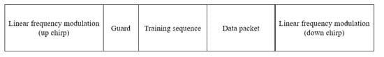
Figure 1.
The packet structure.
The matched filter used for CSS demodulation compares the two chirp signals. If the received signal is expressed as and is divided into one symbol length, it can be described as . The cross-correlation between and the two chirps is checked, and the bit to the larger chirp is determined. Equation (5) expresses the matched filter algorithm:
where is the value converted to the fast Fourier transform (FFT) of the input signal; is the maximum value of cross-correlation between and ; is the maximum value of cross-correlation between and ; and is the demodulated bits. If , the bits are demodulated by 0, else the bits are demodulated by 1.
A CSS modulation block diagram is shown in Figure 2. The signal that passes through a channel leaves only the band energy using a band pass filter (BPF) and uses preamble for fine synchronization of the data packet. Finally, two matched filters are used to demodulate the bit information.
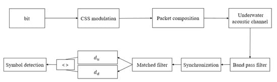
Figure 2.
Block diagram of a conventional chirp spread spectrum (CSS) method.
3. Differential Chirp Spread Spectrum
The differential chirp spread spectrum (DCSS) method, combining differential coding and CSS methods, is proposed here. Differential coding is encoded using the previous bit and current bit’s exclusive or (XOR) operation [28]. When the original bit is , the differential coding bit is expressed as
where is differential encoding bit and N is the number of bits. is called the initial bit, and it is set to either 0 or 1. The differential encoding bits are decoded through XOR operation, so they can be decoded into original bits. The signal only uses differential encoding bits and generates the same equation as in Equation (4). This is expressed as
First, the received signal, cut into two symbol lengths, is expressed as . There are four types of matched filters in DCSS. This is expressed as
where is an up chirp that comes after an up chirp; is a down chirp that comes after a down chirp; is an up chirp comes after a down chirp; and is a down chirp come after an up chirp. If the received signal is expressed as and is divided into two symbol lengths, it can be described as . The cross-correlation between and the four symbols are checked, and the bit to the largest symbol is determined. We used these filters for demodulation. That is, in the conventional method, a matched filter is constructed using only one symbol of up or down chirp, but the size of this time–bandwidth product changes because the proposed method uses two symbols. This is expressed as
where is the maximum value of cross-correlation between and ; is the maximum value of cross-correlation between and ; is the maximum value of cross-correlation between and ; and is the maximum value of cross-correlation between and . When have a maximum value, the bit is demodulated by 0, and when have the maximum value, the bit is demodulated by 1.
The DCSS method is shown in Figure 3. Although it is similar to the overall common CSS method, it uses differential encoding in the modulation process and two symbols at the receiver. The time–bandwidth product doubles because the chirp of the two symbols is determined whether there is a change in the chirp or not, and the matched filter is applied using two symbols. As the time–bandwidth product increases, the filter output increases, and it is possible to have better performance even if the SNR becomes worse.
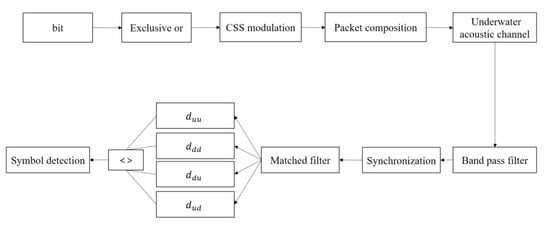
Figure 3.
Block diagram of the differential chirp spread spectrum (DCSS) method.
4. Simulation
The simulation performed two types of verification: performance according to SNR and performance in Doppler effects. In other words, simulations showed how the time–bandwidth product changes with the DCSS rather than CSS, and the performance of the two methods was also compared in the Doppler shift.
The parameters used in the simulations are represented in Table 2. Through repeated simulations with these parameters, the simulation was conducted with a total of bits. The results are shown in Figure 4a,b. Figure 4a shows the difference in performance of each method according to the SNR. First, the black square is the conventional CSS method with a transmission rate of 50 bps, and the blue circle is the conventional CSS method with a transmission rate of 100 bps. Assuming that the TBP of 100 bps is 1, the TBP is 2 because the TBP is doubled at 50 bps, where the transmission rate is half. Finally, the red scissors are a DCSS method with a transmission rate of 100 bps, and since the matching filter is formed using two symbols, the TBP becomes 2. Figure 4b shows the error accumulation rate according to the speed. This was used to analyze the performance according to the error accumulation degree in the Doppler environment. The blue dotted line is 0 knots, the red solid line is 2 knots and the black dashed line is 4 knots; the circled line is the conventional method and the proposed method is indicated by the scissors mark. It was confirmed that the performance of the proposed method in the figure is more durable due to Doppler than the conventional method.
Table 2.
Simulation parameters.
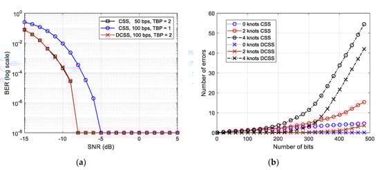
Figure 4.
Results of the simulation: (a) performance according to the signal-to-noise ratio (SNR) and (b) performance according to Doppler.
Figure 4a shows the performance of each method according to the SNR for simulations conducted at intervals of 1 dB from an SNR of −15 dB to 5 dB. The traditional CSS method began to generate errors below −5 dB, and the proposed method was found to be near −8 dB. The CSS method proposed had a BER of near −10 dB, and the proposed method had a BER of about near −13 dB, which improves the SNR by about 3 dB compared to the CSS method.
Figure 4b shows the analysis of the performance of each approach in the environment with Doppler effects. First, we assumed a situation in which the transceiver was moved away at a speed of 4 knots and in which the SNR is 0 dB. In this situation, the x-axis is expressed in the order of bits listed in the packet, and the cumulative error by bits is expressed on the y-axis. This determines the performance by increasing the error rate due to the effects of Doppler as the slope of the graph increased. The cause of the increase in error rate was confirmed by Doppler. The error was accumulated by the motive and the error bit was increased by the bit stream. The CSS method clearly showed that the errors increased after the 200th bit stream. Next, the DCSS method was found to have a significantly more stable performance than the CSS method, although some errors were accumulated after the 200th bit stream. This confirmed that the proposed method with increased time–bandwidth product cost was stronger for noise and Doppler than the conventional method.
5. Experiment
5.1. Lake Trial
We conducted a lake trial using a proven signal through simulation. The experiment was conducted in May 2020, in South Korea. The experiment was conducted slightly differently on different dates.
The experimental configurations are shown in Table 3. The transmitter used Neptune D/17/BB, and the receiver used Reson TC-4032 [29,30]. The communication method was single-input single-output (SISO) communication. There were two bases in the center of the lake that fixed the transmitter and receiver, and one unfixed barge. The distance between the bases was fixed at about 180 m. There was continuous travel by wind or by engine power. In the experimental configuration, the distance between the transceiver was fixed at about 180 m in Experiments 1 and 3, and the barge moved unfixed between 100 m and 300 m in the 2nd experiment. The depth of the lake was about 50 m, and the receiver was always fixed at a depth of about 25 m. The depth of the transmitter was varied: 20 m on the 1st, 10 m on the 2nd and 5 m on the 3rd experiment.
Table 3.
Parameters for the lake experiment from May, 2020.
To analyze the signals, an understanding of the channel environment is essential. We analyzed the channel characteristics of each channel at which the signal was transmitted in order to determine whether there was a change in performance according to the channel impulse response (CIR). The channel measured the LFM pings with a length of 0.128 ms by repeatedly transmitting 200 times. A measured CIR is expressed as
where is the received signal; is the transmitted signal; and is the CIR. In Equation (10), is cut to the length of the ping and is expressed again in matrix , which is expressed as
where q is the time delay and n is a time instant. We can calculate the delay in Doppler spread function by . The FFT of gives a spreading function, as expressed by Equation (12),
and summation of the delay axis provides an estimate of the Doppler spectrum :
The characteristics of each experiment are expressed in Figure 5, Figure 6 and Figure 7. Figure 5a, Figure 6a and Figure 7a represent the CIR of each experiment; Figure 5b, Figure 6b and Figure 7b represents the delay-Doppler spread spectrum of each experiment; Figure 5c, Figure 6c and Figure 7c is the power delay profile; and Figure 5d, Figure 6d and Figure 7d is the Doppler power spectrum.
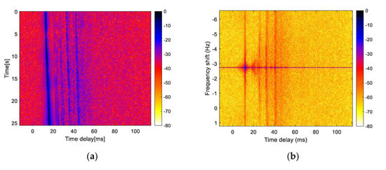
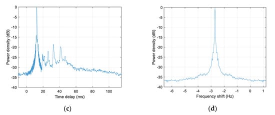
Figure 5.
The lake-measured channel in the 1st experiment: (a) CIR; (b) delay-Doppler spread spectrum; (c) power delay profile; (d) Doppler power spectrum.
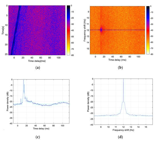
Figure 6.
The lake-measured channel in the 2nd experiment: (a) CIR; (b) delay-Doppler spread spectrum; (c) power delay profile; (d) Doppler power spectrum.
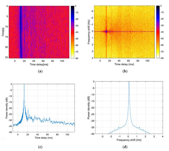
Figure 7.
The lake-measured channel in the 3rd experiment: (a) CIR; (b) delay-Doppler spread spectrum; (c) power delay profile; (d) Doppler power spectrum.
The 1st experiment had a number of multipaths, and a slight tilt was seen in the CIR. The channel was not constant, and a slight tilt was seen, so there was some time variance. The delay-Doppler spread spectrum showed that it moved to −0.49 knot with a Doppler frequency of about −2.7 Hz. In the 2nd experiment, the receiver was fixed in the same position, but the transmitter was placed in a barge. So, the 2nd had 2 multipaths and a big tilt was seen in the CIR. The delay-Doppler spread spectrum showed that it moved to 2.18 knots with a Doppler frequency of about 12 Hz. In the 3rd experiment, the location was the same as in the 1st experiment, but there was a difference in multipath, depending on the depth of the water. In the 3rd experiment, the CIR had only 1 multipath and a SNR similar to the 1st experiment. The delay-Doppler spread spectrum showed that it moved to knots with a Doppler frequency of about 0.02 Hz.
Through the channels analyzed for each experiment, we compared the performance of the CSS and DCSS techniques and also analyzed in which environment the chirp-based communication was stronger. First, the communication performance is represented in Table 4. The results shown in Table 4 indicate that the performance in the 3rd experiment was the best and the 1st experiment was the worst. The spectrograms of the received signals on each experiment are shown in Figure 8.
Table 4.
Lake experiment results.
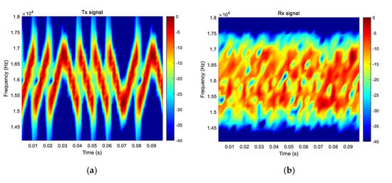
Figure 8.
The spectrogram (a) of the transmitted signal; (b) received signal on the 1st experiment; (c) received signal on the 2nd experiment; (d) received signal on the 3rd experiment.
According to the channel measured on the 1st experiment, the symbolic length of the signal with a data rate of 100 bps was 10 ms, which caused inter-symbol interference (ISI) to be generated and reduced the output of the matched filter; the SNR was 6.361 dB. In this situation, increasing the output of the matched filter by increasing the time–bandwidth product should improve the performance. The existing CSS method had a BER of 0.1696, but the proposed DCSS method showed a significant improvement in performance with 0.03570. In the 2nd experiment, Doppler existed because the transmitter was not fixed, and the SNR was also lower than in the other experiments. The multipath was very small in size, so only the direct path was clearly identified; the SNR was 1.879 dB. The existing method had a BER of 0.1071, and the proposed method had a BER of 0.0238 on the following channels. This shows that the proposed method also leads to improved performance in terms of Doppler effects; however, it was possible to infer that performance was improved even by a low SNR. Finally, the 3rd experiment did not have many multipaths, and the SNR was the highest among the three experiments of the study. Doppler was limited because both the transmitter and receiver were fixed; the SNR was 8.067 dB. Both the channel’s time volatility and SNR were better than on the other experiments, so the existing method also had a fairly good performance at 0.00895. The proposed method further improved this and had a 0 BER.
5.2. Sea Trial
A sea experiment was conducted in October 2018 in the East Sea, South Korea. The experimental configuration was constructed as shown in Figure 9, and the experiment was conducted from a vertical line array (VLA) of about 90 km. The water depth was ~1500 m. The experimental configurations are shown in Table 5. The source, a Neptune T-161 projector, was located ~200 m below the sea surface and transmitted signals over the 1.8 kHz centered frequency [31]. The 16-element receiving hydrophones were located 179–221 m away under a sea surface buoy. This is a vertical line array (VLA) with an inter-element spacing of 2 m. The collected acoustic data, as well as some of the collected oceanographic data, were self-recorded, providing the VLA coordinates by continuous real-time monitoring via a telemetry buoy; this is represented in Figure 9a. The map in Figure 9b shows the geography of the East Sea. In Figure 9b, the circle is the receiver, the star shape represents the position of the transmitter and the line drawing between the star and circle is the chip route measured by a global positioning system (GPS).
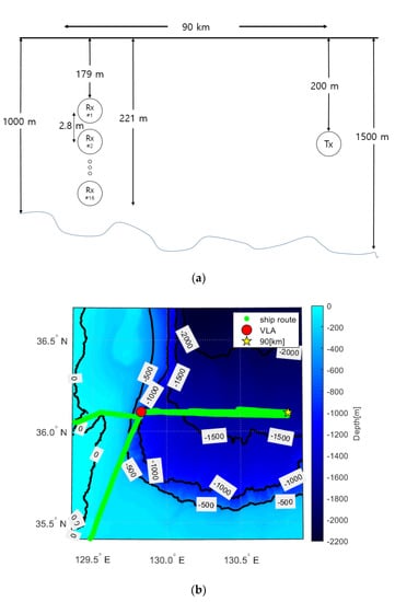
Figure 9.
Sea experiment configuration: (a) configuration view from the side; (b) configuration view from above.
Table 5.
Parameters for the sea experiment.
Before checking the results of the sea experiment, the channel was measured. The CIR is shown in Figure 10. The channel has one big multipath, which was reached before the main path. The delay was about 50 ms and there was about −3.24 Hz Doppler.
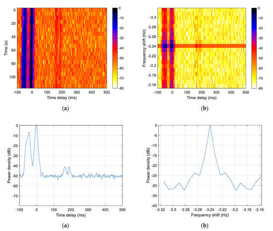
Figure 10.
The sea-measured channel at 90 km: (a) CIR; (b) delay-Doppler spread spectrum; (c) power delay profile; (d) Doppler power spectrum.
The spectrogram of the signal received from the sea experiment is shown in Figure 11. In the sea experiment, the SNR was measured as very low, about −6.51 dB. The reason that the SNR in the channel impulse response looks better than that of the lake experiment is the effect of the increase in the matched filter output value according to the length of the LFM. In the experiment, the BER for the modified conventional method was , and the BER for the proposed method was 0 BER. It was thereby confirmed that the proposed method for long-distance communication shows good improvement on performance.
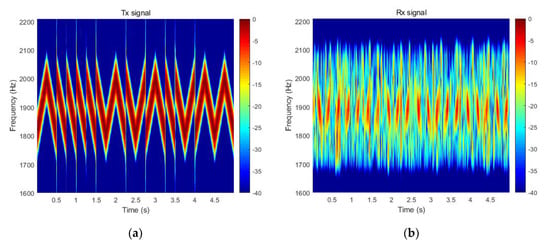
Figure 11.
The spectrogram of (a) the transmitted signal and (b) the received signal.
6. Conclusions
CSS communication is a good modulation to use wideband in a variety of environments. We explained how to improve performance when using the duplication method using the matched filter in the CSS method. If the size of the matched filter is doubled by applying a differential coding method, performance is improved by taking advantage of the fact that the time–bandwidth product cost increases. The simulation of the SNR proved that performance improved by about 3 dB and confirmed that performance was also improved in the environment where the Doppler shift occurred. In lake and sea experiments, we confirmed that the proposed method improved performance. The lake experiment confirmed that the performance improves significantly when there are multipath and Doppler effects, and the sea experiment confirmed the performance improvement in long-range communication of 90 km. Next, a study is needed on the possibility of improving both the bit rate and performance by utilizing differential coding in multiband CSS communication.
Author Contributions
All authors contributed significantly to the work presented in this manuscript. J.L. and K.K. proposed the method described here; J.L., J.A. and K.K. conceived and designed the experiments; J.L., H.-i.R. and J.A. performed the experiments and analyzed the data. All authors have read and agreed to the published version of the manuscript.
Funding
This research received no external funding.
Conflicts of Interest
The authors declare no conflict of interest.
References
- Stojanovic, M. Recent advances in high-speed underwater acoustic communication. IEEE J. Ocean. Eng. 1996, 21, 125–136. [Google Scholar] [CrossRef]
- Stojanovic, M. Acoustic (underwater) communication. In Wiley Encyclopedia of Telecommunication; John Wiely & Son: New York, NY, USA, 2003. [Google Scholar]
- Mosca, F.; Matte, G.; Mingnard, V.; Rioblanc, M. Low frequency source for very long range underwater communication. In Proceedings of the 2013 OCEANS—San Diego, San Diego, CA, USA, 23–27 September 2013; pp. 1–5. [Google Scholar]
- Shimura, T.; Ochi, H.; Wantabe, Y.; Hattori, T. Time reversal communication in deep ocean—Result of recent experiments. In Proceedings of the 2011 IEEE Symposium on Underwater Technology and Workshop on Scientific Use of Submarine Cables and Related Technologies, Tokyo, Japan, 5–8 April 2011; pp. 1–5. [Google Scholar]
- Song, H.C. Acoustic communication in deep water exploiting multiple beams with a horizontal array. J. Acoust. Soc. Am. 2012, 132, EL81–EL87. [Google Scholar] [CrossRef] [PubMed]
- Liu, Z.; Yoo, K.; Yang, T.C.; Cho, S.E.; Song, H.C.; Ensberg, D.E. Long-Range Double-Differentially Coded Spread-Spectrum Acoustic Communications with a Towed Array. IEEE J. Ocean. Eng. 2013, 39, 482–490. [Google Scholar] [CrossRef]
- Song, H.C.; Hodgkiss, W.S. Diversity combining for long-range acoustic communication in deep water. J. Acoust. Soc. Am. 2012, 132, EL68–EL73. [Google Scholar] [CrossRef] [PubMed]
- Loubet, G.; Capellano, V.; Filipiak, R. Underwater spread-spectrum communications. In Proceedings of the Oceans’97 MTS/IEEE Conference, Halifax, NS, Canada, 6–9 October 1997; pp. 574–579. [Google Scholar]
- Freitag, L.; Stojanovic, M.; Johnson, M. Analysis of Channel Effects on Direct Sequence and Frequency Hopped Spread Spectrum Acoustic Communication. IEEE J. Ocean. Eng. 2001, 26, 586–593. [Google Scholar] [CrossRef]
- Zhou, F.; Liu, B.; Nie, D.; Yang, G.; Zhang, W.; Ma, D. M-ary Cyclic Shift Keying Spread Spectrum Underwater Acoustic Communications Based on Virtual Time-Reversal Mirror. Sensors 2019, 19, 3577. [Google Scholar] [CrossRef] [PubMed]
- Lam, A.W.; Tantaratana, S. Theory and Applications of Spread-Spectrum Systems a Self-Study Course, 1st ed.; Institute of Electrical and Electronics Engineers: Piscataway, NJ, USA, 1994; pp. 27–76. [Google Scholar]
- Urick, R.J. Principle of Underwater Sound, 3rd ed.; McGraw-Hill Book Company: New York, NY, USA, 1996; pp. 99–197. [Google Scholar]
- Andreja, R.; Rameez, A.; Tolga, M.E.; John, G.P.; Milica, S. Adaptive OFDM Modulation for Underwater Acoustic Communication: Design Consideration and Experimental Result. IEEE J. Ocean. Eng. 2013, 39, 357–370. [Google Scholar] [CrossRef]
- Taehyuk, K.; Song, H.C.; Hodgkiss, W.S. Multi-carriers Synthetic Aperture Communication in Shallow Water: Experimental results. J. Acoust. Soc. Am. 2011, 130, 3797–3802. [Google Scholar] [CrossRef]
- Kai, T.; Tolgra, M.D.; Stojanovic, M.; John, G.P. Multiple Resampling Receiver Design for OFDM over Doppler Distorted Underwater Acoustic Channels. IEEE J. Ocean. Eng. 2013, 38, 333–346. [Google Scholar] [CrossRef]
- Leus, P.; Van Walree, P. Multiband OFDM for Covert Acoustic Communication. Sel. Areas Commun. IEEE J. 2008, 26, 1662–1673. [Google Scholar] [CrossRef]
- Du, P.; Zhu, X.; Li, Y. Direct Sequence Spread Spectrum Underwater Acoustic Communication Based on Differential Correlation Detector. In Proceedings of the 2018 IEEE International Conference on Signal Processing, Communications and Computing (ICSPCC), Qingdao, China, 14–16 September 2018; pp. 1–5. [Google Scholar]
- Yang, T.C.; Yang, W.B. Performance Analysis of Direct Sequence Spread Spectrum Underwater Acoustic Communication with Low Signal to Noise Ratio Input Signals. J. Acoust. Soc. Am. 2008, 123, 842–855. [Google Scholar] [CrossRef] [PubMed]
- Qu, F.; Yang, L.; Yang, T.C. High reliability direct-sequence spread spectrum for underwater acoustic communications. In Proceedings of the 2009 OCEANS, Biloxi, MS, USA, 26–29 October 2009; pp. 1–6. [Google Scholar]
- Zhan, C.; Xu, F.; Hu, X. Parallel combinatory multicarrier frequency-hopped spread spectrum for long range and shallow underwater acoustic communications. In Proceedings of the MTS/IEEE OCEANS—Bergen, Bergen, Norway, 10–14 June 2013; pp. 1–7. [Google Scholar]
- Yang, W. High-Frequency FH-FSK Underwater Acoustic Communications: The Environmental Effect and Signal Processing. In AIP Conference Proceedings; AIP Publishing: College Park, MD, USA, 2004; Volume 728, pp. 106–113. [Google Scholar]
- Kaminsky, E.J.; Simanjuntak, L. Chirp slope keying for underwater communications. In Proceedings of the SPIE Sensors, and Command, Control, Communication, and Intelligence (C31) Technologies for Homeland Security and Homeland Defense VI Conference, Orlando, FL, USA, 28 March–1 April 2005; pp. 894–905. [Google Scholar]
- En, C.; Xiaoyang, L.; Fei, Y. Multiuser underwater acoustic communication based on multicarrier-multiple chirp rate shift keying. In Proceedings of the OCEANS 2014—TAIPEI, Taipei, Taiwan, 7–10 April 201; pp. 1–5.
- Demirors, E.; Melodia, T. Chirp-based LPD/LPI underwater acoustic communications with code-time-frequency multidimensional spreading. In Proceedings of the 11th ACM International Conference on Underwater Networks & Systems, Shanghai, China, 24–26 October 2016; pp. 1–6. [Google Scholar]
- Transter, W.H.; Shanmugan, K.S.; Rapport, T.S.; Kobar, K.L. Principle of Communication Systems Simulation with Wireless Application; Prentice Hall: Upper Saddle River, NJ, USA, 2003; Chapter 3. [Google Scholar]
- Van Walree, P.; Socheleau, F.X.; Otnes, R.; Jenserud, T. The Watermark Benchmark for Underwater Acoustic Modulation Schemes. IEEE J. Ocean. Eng. 2017, 42, 1007–1018. [Google Scholar] [CrossRef]
- Van Walree, P. Channel Sounding for Acoustic Communication: Techniques and Shallow-Water Example; Forsvarets Forskningsinstitutt: Kjeller, Norway, 2011; pp. 9–22. [Google Scholar]
- Mano, M.M. Digital Design, 3rd ed.; Prentice Hall: Upper Saddle River, NJ, USA, 2007; Chapter 3. [Google Scholar]
- Neptune Sonar. Available online: http://www.neptune-sonar.co.uk/wp-content/uploads/2016/03/Model-D17BB.pdf (accessed on 30 October 2020).
- Reson Hydrophone. Available online: https://www.m-b-t.com/fileadmin/redakteur/Ozeanographie/Hydrophone/Produktblaetter/TC4032.pdf (accessed on 8 September 2018).
- Neptune Sonar. Available online: http://www.neptune-sonar.co.uk/wp-content/uploads/2016/03/Model-T161.pdf (accessed on 30 October 2020).
Publisher’s Note: MDPI stays neutral with regard to jurisdictional claims in published maps and institutional affiliations. |
© 2020 by the authors. Licensee MDPI, Basel, Switzerland. This article is an open access article distributed under the terms and conditions of the Creative Commons Attribution (CC BY) license (http://creativecommons.org/licenses/by/4.0/).