Position-Dependent Stability Prediction for Multi-Axis Milling of the Thin-Walled Component with a Curved Surface

Abstract

Time-varying dynamic behaviors are essential to investigate the stability in the thin-walled workpiece milling process, which is usually affected by material removal and position-dependent characteristics of the workpiece along with the tool feed direction. To predict the milling stability with position-dependent, thin-walled component multi-axis milling, an improved structural dynamic modification method with variable mass is proposed in the paper. Firstly, the extraction of multi-axis milling material and the removal process of thin-walled parts with a complex curved surface and variable thickness is completed with CAM software. Then, the material removal of one cutting path as a modification of the structure is divided into multi-cutting steps with equal length to obtain the corrected FRFs in the machining process on the basis of the extended Sherman-Morrison-Woodbury formula. Furthermore, the dynamic characteristics of the initial un-machined workpiece and final machined workpiece are calculated by both experimental modal analysis and FEM. Finally, the multi-axis milling stability is predicted using the extended numerical integrated method, and an aero-engine blade is used to validate the accuracy and effectiveness of the proposed method for multi-axis milling molding parts.

1. Introduction

With the rapid development in the manufacturing sector, thin-walled parts with a complex curved surface and variable thickness are widely used in the aerospace, automobile, mold, and other industries because of the advantages of the lightweight and high-specific strength. However, these thin-walled parts have low stiffness, which triggers serious vibrational problems in the machining process. Therefore, the improvement of the processing efficiency and ensuring processing quality remain hot topics for both academia and the industry. In the multi-axis milling process of such parts, the selection of existing cutting parameters and the formulation of processing technology relies heavily on the actual processing experience; and the parameters selected as such tend to be conservative. Although it can ensure the processing quality, the low efficiency and long production cycle cannot meet the needs of the manufacturing industry. 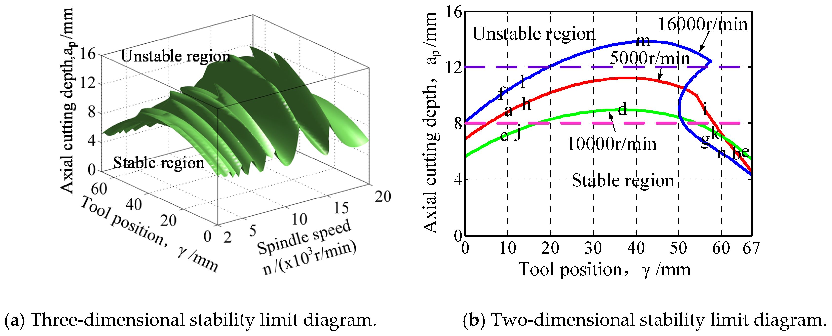Under the premise of ensuring the processing quality, it is an urgent problem to select larger cutting parameters [1,2], where the traditional two degrees’ freedom chatter model is expanded and a three degrees freedom chatter model is established. The stability limit diagram of multi-axis milling is obtained by the taking spindle speed, axial cutting depth, and radial cutting depth as coordinate axes, so as to optimize process parameters and improve machining efficiency.

Multi-axis milling is a complex machining process in that the workpiece structure is complex and the tool movement is changeable, which leads to the change of machining parameters. Thereby, the majority of research on multi-axis milling can mainly be divided into three categories, multi-axis milling force modeling, dynamic stability analysis, and the tool path plan. All these categories have been studied extensively. Firstly, Ozturk et al. [3] presented a model for calculating the cutting force in five-axis milling, in which the cutting force coefficient was obtained by the transformation of the right angle. Additionally, the influence of the inclination angle was also included in the model. Tsai et al. [4] developed a cutting force calculation model through geometric analysis, in which the relationship between the un-deformed chip thickness, tool front angle, cutting speed, shear plane, and chip flow angle were described in detail. The three-dimensional cutting force in the tool coordinate system was obtained with the minimum energy method. On the basis of the Johnson–Cook theory, Saffar et al. [5] predicted the cutting force of the end milling cutter in the milling process with FEM. On the basis of the analysis of tool motion, Sun et al. [6] proposed an instantaneous cutting force calculation model in the case of the existence of tool eccentricity in the process of five-axis milling. Recently, Tunc et al. [7] developed a cutting force model of multi-axis milling operations, which was calculated by using a new numerical method of the engagement boundary determination approach. Ozkirimli et al. [8] used the zeroth-order approximation frequency domain method to predict the stability of the cutting tool by considering the process damping effect. A generalized cutting forces model of the five-axis milling process is proposed, which can be applied for an arbitrary mill geometry in multi-axis milling as well as three-axis milling and two-and-a-half-axis milling [9]. Liu et al. [10] established a tool path generation method for the five-axis flank milling of pockets based on the constraints of cutting force and kinematics of machine tools. Most of the literature mentioned above assumed that the tool was rigid or neglected the weak rigidity of the workpiece. Meanwhile, the cutting force modeling has been relatively mature. However, most of the cutting force models are specific to certain tool forms only, such as end milling cutters, and ball milling cutters, and so forth, without considering the influence of time-varying parameters. Therefore, the establishment of a multi-axis milling cutting force time-varying parameter model is crucial.

Many experts and scholars have also conducted extensive research on the dynamic characteristics of thin-walled milling. For the dynamic characteristic extraction step, Yue et al. [11] summarized the current state of the stability prediction for the thin-walled components milling system and presented the variety of extraction methods of dynamic characteristics. This can be roughly classified into two categories: one is a function of time and space considering material removal and position dependence, and the other is a constant. Alternatively, some scholars assume that when the radial cutting depth is very small, the effect of material removal on the dynamic characteristics of thin-walled parts is small and can be ignored accordingly. In the frequency domain methods [12,13] and in time do main methods [14,15], the dynamic characteristics of the workpiece in the machining process are position-dependent. Later, Bravo et al. [16] obtained the 3D-SLD with the hypothesis that both the cutter and the workpiece were flexible and the deformation was large in three-axis perimeter milling. Wan et al. [17] used the lowest envelope method to deal with a similar problem, which may cause some prediction errors when the modes of the workpiece are not well separated. Mostly, the above mentioned methods used the impact test to obtain the modal parameters. Therewith, Mane et al. [18] built the finite element model of the workpiece and considered the influence of gyroscopic effect and bearing stiffness on the stability in the milling process of thin-walled parts. Tang et al. [19] concentrated on the effect of position-dependent characteristics for the thin-walled parts dynamic, built a 3D-SLD model of thin-walled parts milling, and optimized the maximum removal rate of materials on the basis of the assumption that the dynamic characteristics of thin-walled parts were unchanged in the milling process. The dynamic characteristics were changed by a new device proposed in Kolluru et al. [20] in the milling process of thin-walled parts, and the modal quality and stiffness improved. Lately, an undetermined coefficient method was employed in the work of Guo et al. [21] to identify the modal parameter for the general cutter system of three axis half immersion milling in a horizontal plane.

However, as for a thin-walled workpiece, the effect of material removal and position-dependent characteristics of the cutter on dynamic characteristics is a non-negligible factor; the stability also changes during the machining process. In the early years, Thevenot et al. [22] studied the variation of the dynamic characteristics of thin-walled parts with respect to tool position. Later, they took the material removal into consideration to construct 3D-SLD using FEM [23]. Campa et al. [24] presented a stability model of milling systems in the tool axis direction with bull-nose end mills. According to Biermann et al. [25], the modal parameters can be interpolated to obtain the dynamics of workpieces, in which the dynamic characteristics changed remarkably during the material removal process. Brecher et al. [26] calculated the modal parameters of the machine tool along arbitrary tool paths in different discrete axis positions, where an interpolation strategy was applied. Zhou et al. [27] developed a stability prediction analytical model of aero-engine casings in bull-nose end milling. Shi et al. [28] firstly derived a new computational model by dividing the workpiece into the removed part and remaining part with the Ritz method and obtained a more accurate prediction of stability. Song et al. [29] employed the FEM method with the material removal effect to construct a 3D-SLD to achieve the optimal cutting conditions during the milling process. The materials can be removed with uniform thickness using the five-axis flank milling tool by Shao et al. [30] while considering the dynamic characteristics of the machine tool and the milling force constraint. Yan et al. [31] optimized the multi-axis machining strategy on the basis of the thought of variable depth-of-cut machining for thin-walled workpieces. Bierman et al. [32] obtained the effect of material removal on the dynamic characteristics of thin-walled parts in the milling process by the hammering method and established the stability limit diagram. Song et al. [33] proposed a structural dynamic modification method with equal mass to predict the dynamic stability of the thin-walled workpiece milling process. Based on the Ad-ams-Bashforth scheme, a numerical difference method is proposed by Dun et al. [34] with considering material removal and position dependence for thin-walled workpiece stability prediction. All the above studies are based on the equal thickness thin-walled workpiece, in which material removal is conducted on an equal-mass basis. Therefore, as an extension, Shi et al. [35] studied the dynamic response of a thin-walled component with variable thickness in the milling process.

Nonetheless, the existing research mostly focuses on the three-axis side milling of thin-walled parts; the tool structure is simple, the workpiece is relatively regular, most of its parts are cuboid thin-walled parts, few of which involve the multi-axis milling process of thin-walled parts with a complex curved surface and variable thickness. Wu et al. [36] developed a cyclic symmetry analysis method to solve the dynamic characteristic issues of the thin-walled integral impeller. In the study, Wu assumed that the dynamic characteristic of the integral impeller was approximately equal to a single blade. Nikolaev et al. [37] obtained the dynamic characteristics of a jet-engine blade by the modal experiment while using a time-domain method to evaluate a chatter-free milling mode. Tuysuz et al. [38] presented a novel method of reduced-order workpiece dynamic parameters updated model for the thin-walled parts in the frequency domain and time domain, based on the perturbation and reduced-order substructuring methods. The dynamics of the workpiece in processing was predicted by using the structural dynamic modification method [39]. However, there is no in-depth research regarding the dynamic characteristics of the impeller. In the actual production and machining process, the processed thin-walled parts are mostly complex curved surfaces, and variable thickness is more common. In addition, most of the traditional methods (such as FEM or modal test) in the literature for the instantaneous dynamics prediction need to re-build and re-mesh the FEM model at each cutting step, which proves time-consuming and inefficient. Therefore, it is necessary to study the dynamic characteristics of multi-axis milling of thin-walled parts with a complex surface and variable thickness.

Aiming at tackling the limitation, this paper adopts a structural dynamic modification method to predict the stability of a multi-axis milling thin-walled workpiece with variable mass removal. First, a time-varying parameter system model for multi-axis milling of thin-walled parts with a complex curved surface and variable thickness is established. Second, the instantaneous dynamic characteristics of workpiece processing are obtained using the extended Sherman–Morrison–Woodbury method with the dynamic characteristic parameters of the workpiece before and after the machining is completed. Subsequently, the variation curve of the dynamic characteristics of the workpiece in the process of machining with the cutting path is obtained using the least squares method. Finally, the stability of multi-axis milling is predicted using the extended numerical integrated method, and a typical multi-axis milling molding part of the aero-engine blade is employed to verify the proposed method.

The rest of the paper is organized as follows. Section 2 presents a dynamic model with variable parameters in the multi-axis milling system and obtains the material removal process. Section 3 identifies the time-varying parameters based on the extended Sherman–Morrison–Woodbury formula. Section 4 introduces the experimental setup and procedure. Section 5 carries out the verification of the theoretical results and case analysis. Finally, the conclusions are given in Section 6.

2. Dynamic Model of Complex Curved Surface Thin-Walled Parts with Variable Thickness

2.1. Time-Varying Parameters Model of Multi-Axis Milling

The machining process of thin-walled parts with a complex curved surface and variable thickness during multi-axis milling is complicated in that the parameters and the tool movement are subject to change. Therefore, it tends to be difficult to directly apply the traditional three-axis milling stability prediction theory to the multi-axis milling process. This section establishes a dynamic model with time-varying parameters of thin-walled parts with a complex curved surface and variable thickness during multi-axis milling. In Figure 1, we consider to have a degree of freedom assuming a rigid spindle toolset because of the greater flexibility of the structure. To accurately describe the relative motion of the tool and the workpiece, three coordinate systems, Global Coordinate System (GCS), Feed Cross-feed Normal System (FCN), and Tool Coordinate System (TCS) are employed here as shown in Figure 1.

In the milling process, the time-varying cutting force f_N(t) excites the workpiece, so that the workpiece has a dynamic displacement N(t) along the surface normal. Material removal affects the system dynamics, and the workpiece dynamic characteristic changes along the cutting path. Hence, the corresponding control equation of time-varying parameters system is [40]

$$\ddot{N}(t)+2\zeta (t){\omega }_{\mathrm{n}}(t)\dot{N}(t)+{\omega }_{\mathrm{n}}^2(t)N(t)=f_N(t)/m(t).$$

(1)

where

• N(t)—the displacement of the point along the surface normal on the surface of the workpiece,
• ζ(t)—the modal damping ratio of the workpiece and ζ(t) = c/[2(mk)^1/2],
• ω_n(t)—the natural frequency of the workpiece and ω_n(t) = [k/m]^1/2,
• m, c, and k- are the position-dependent parameters of the modal mass, the modal damping, and the modal stiffness of the workpiece, respectively.

Due to the feed motion of the tool, the parameters m, c, and k are the functions of time, that is m(t), c(t), and k(t). f_N(t) is the cutting force exerted on the workpiece along the workpiece surface normal. Note that the numerator f_N(t) on the right side of Equation (1) consists of two parts, f_N(t) = p(t) + f(t), where f(t) is the static cutting force acting on the workpiece. This mainly causes the forced vibration of the workpiece, and p(t) is the dynamic cutting force acting on the workpiece, which is produced by the regenerative effect in the cutting process. For the multi-axis milling process, modeling the cutting model is the essential focus for further analysis, due to the complex material removal process. This problem will be discussed in the following section.

During the semi-finishing and finishing of the blade, the material removal has a great influence on the blade dynamics. For a specified cutting process, the variation of the tool rake angle and roll angle is shown in Figure 2, according to Ju et al. [41], by simulation method. As can be seen, the rake angle and roll angle of the tool change continuously with the cutting position in the cutting process. The roll angle stays positive while gradually decreasing from 70° to 50°. Initially, the rake angle is negative but gradually increases from −40° to 20° as the milling operation proceeds. This represents the typical characteristics of the multi-axis milling operation.

In the multi-axis milling process, the dynamic cutting thickness of the jth cutter teeth is shown in Figure 3, where

• W—the static cutting thickness,
• n_TCS(t)—the vibration displacement generated by the current cutter tooth cutting,
• τ—the tooth passing period and τ = 2π/(N_tΩ), and
• N_t—the number of cutter teeth,
• Ω—the angular velocity of the cutting tool.

In Figure 3, the dynamic cutting thickness along the surface normal of the tool can be expressed as

$$h_{j,\mathrm{d}}(z,t)=n_{\mathrm{TCS}}(t)-n_{\mathrm{TCS}}(t-\tau )$$

(2)

In the tool coordinate system TCS, Equation (2) can be expressed as

$$h_{j,\mathrm{d}}(z,t)=\Delta x\sin {\phi }_j\left(z,t\right)\sin k(z)+\Delta y\cos {\phi }_j\left(z,t\right)\sin k(z)-\Delta z\cos k(z)$$

(3)

where Δx = [x(t) − x(t − τ)], Δy = [y(t) − y(t − τ)], and Δz = [z(t) − z(t − τ)]. From Ju et al. [41], the relationship between TCS and FCN can be expressed as

$$(x, y, z, 1)=(F, C, N, 1)R_{\mathrm{FCN}\to \mathrm{TCS}}$$

(4)

here R_FCN→TCS is the rotation matrix which from the FCN coordinate system to the TCS coordinate system, which is expressed as

$$R_{\mathrm{FCN}\to \mathrm{TCS}}=\left[\begin{array}{cccc}\cos \alpha & 0& \sin \alpha & 0\\ \sin \alpha \sin \beta & \cos \beta & -\cos \alpha \sin \beta & 0\\ -\sin \alpha \cos \beta & \sin \beta & \cos \alpha \cos \beta & 0\\ 0& 0& 0& 1\end{array}\right]$$

(5)

where α is the rake angle, and β is the roll angle of the tool. Only considering the vibration along the surface normal of the workpiece, thus Equation (4) can be expressed as

$$(\Delta x, \Delta y, \Delta z, 1)=(0,0, \Delta N, 1)R_{\mathrm{FCN}\to \mathrm{TCS}}$$

(6)

where Δx = −ΔN sin α cos β, Δy = ΔNsin β, Δz = ΔN cos α cos β, and ΔN = [N(t − τ) − N(t)]. Hence, the instantaneous dynamic cutting thickness can be expressed as

$${\mathrm{h}}_{i,\mathrm{d}}(t)=\Delta N\mathbf{T}\mathbf{E}$$

(7)

where T = [sin α cos β sin β cos α cos β] is a tool inclination matrix related to the rake angle and the angle. E = [–sin φ_j(z,t) sin κ(z) cos φ_j(z,t) sin κ(z) cos κ(z)]^T is a contact area matrix and the size of which is related to the tool-workpiece contact area in the multi-axis milling process.

When considering the vibration of the workpiece in the surface normal only, the dynamic cutting force obtained in the FCN coordinate system needs to be projected to the tool surface normal N. The dynamic cutting force along the surface normal of the workpiece can be expressed as

$$p(t)=dbd(t)\Delta N(t),$$

(8)

where db is the width of the discrete unit chip without deformation, db = dz/sin κ(z). d(t) is the direction coefficient of the dynamic cutting direction. Submitting Equation (8) into Equation (1), the governing equation of motion with time-varying parameters can be obtained.

2.2. Material Removal Process

Due to the existence of the rake angle and roll angle in the multi-axis milling process, the irregular material removal gradually changes with time. In other words, the material removal amount is generally nonlinear, making it difficult to use the traditional numerical method to calculate the material removal. Using CAM software, here the simulation of the multi-axis milling material removal of thin-walled parts with a complex curved surface and variable thickness is completed, and the material removal process is shown in Figure 4.

With the assistance of CAM software, the material removal process can be programmed to generate the CL files, which is used to extract the moving information of the tool and to obtain the TCS data and the tool axis unit vector in the GCS coordinates. The space envelope of the tool movement (also known as the tool swept volume) is shown in Figure 4a. The generated tool swept volume and the workpiece blank are subjected to the Boolean subtraction operation, and the workpiece can be obtained after machining, as shown in Figure 4b,c. Meanwhile, the removed material can also be obtained in this cutting process, as shown in Figure 4d. The Boolean operations performed are as follows:

Workpiece blank − Workpiece swept volume = End product

(9)

Workpiece blank ∩ Workpiece swept volume = Material removed.

(10)

3. Identification of Time-Varying Parameters

In the milling process of the thin-walled workpiece with a complex curved surface and variable thickness, the dynamic characteristics or frequency response function of the workpiece will change with the tool position and material removal according to Ref. [40]. Meanwhile, the material removal is irregular and the material removal amount generally changes with time. Therefore, the structural dynamic modification method with equivalent mass (SDMM-EM) presented by Ref. [36] is extended to deal with the structural dynamic modification problem with variable mass (SDMM-VM) and identify the instantaneous (or position-dependent) dynamic characteristics of the workpiece.

3.1. Correction of Frequency Response Function

The main concept of the SDMM is to take the material removal process as a structural modification operation for machining the workpiece. Discrete material is removed into many (infinite in limit case) infinitesimal mass elements along the cutting path. When an infinitesimal mass element is removed, the workpiece equivalently performs the one-time structural modification. The dynamic characteristics of the initial workpiece un-machined can be identified utilizing experimental or numerical methods. The dynamic characteristics of the workpiece during machining can then be obtained using the SDMM. It is noted that the SDMM-VM is required because the material removal amount generally changes with time for the multi-axis milling of the workpiece with a complex curved surface. Therefore, the problem is transformed into one that uses the frequency response functions (FRFs) of the initial un-machined workpiece and final machined workpiece to estimate the FRFs of the workpiece during the machining process (named as corrected FRFs).

The multi-axis milling process is divided into n-cutting steps along a cutting path. Each cutting step corresponding to a mass element removed is regarded as a one-time modification to the workpiece shown in Figure 5. Thereby, the results of the dynamic characteristics identified are more accurate as the number of discrete cutting steps increases.

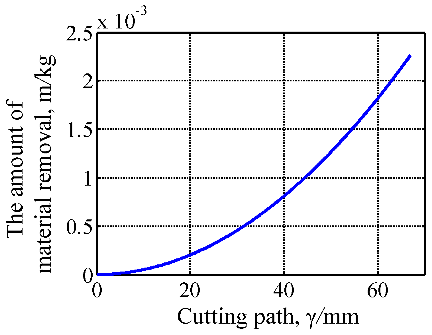
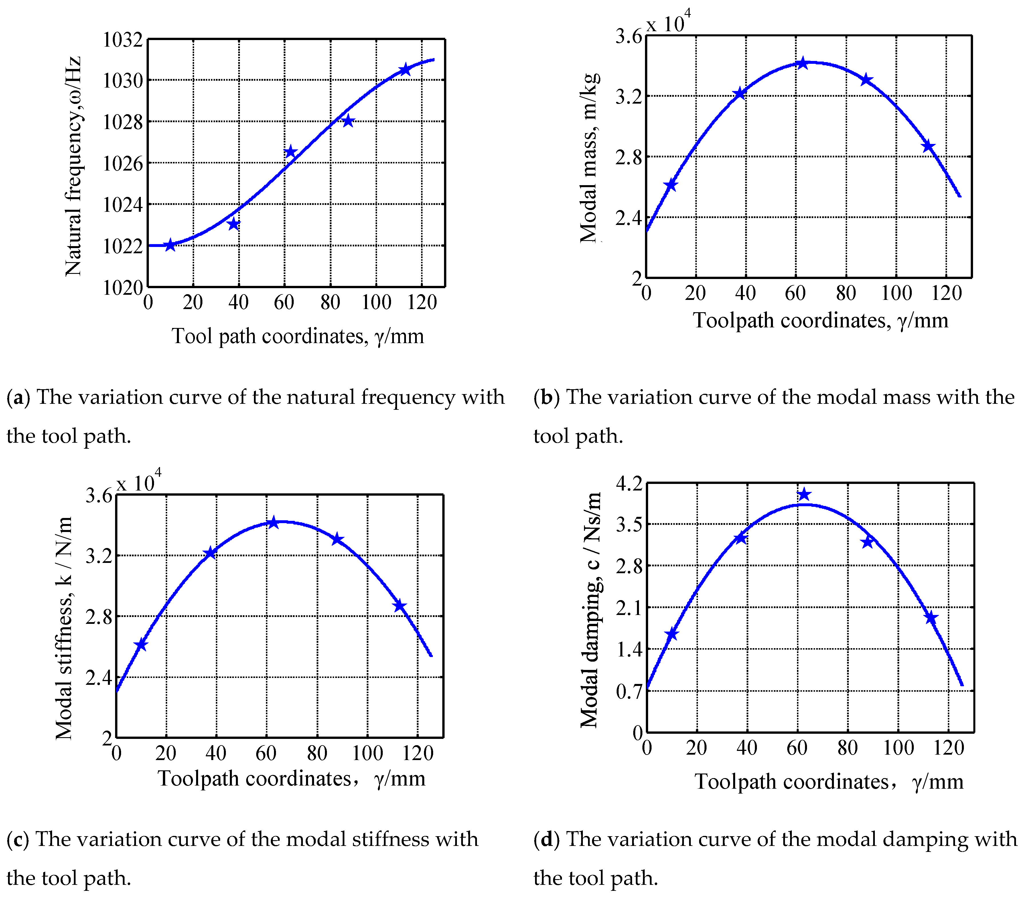
During the multi-axis milling process of the thin-walled parts with a complex curved surface and variable thickness, the shape of material removal is irregular and the amount of material removal is nonlinear, so it is difficult to obtain the modal mass, modal damping, and modal stiffness of the structure. Here, it is assumed that the variations of the modal mass, modal damping, and modal stiffness are proportional to the amount of material removal. That is, the greater amount of material removal there is, the more the variations of modal mass, modal damping, and modal stiffness there are. Therefore, the variations of modal mass, modal damping, and modal stiffness of the structure can be expressed as

$$\Delta m_i=\frac{\delta m_i\left(m_{i,n}-m_{i,0}\right)}{m_{RM}}, \Delta c_i=\frac{\delta m_i\left(c_{i,n}-c_{i,0}\right)}{m_{RM}}, \Delta k_i=\frac{\delta m_i\left(k_{i,n}-k_{i,0}\right)}{m_{RM}}$$

(11)

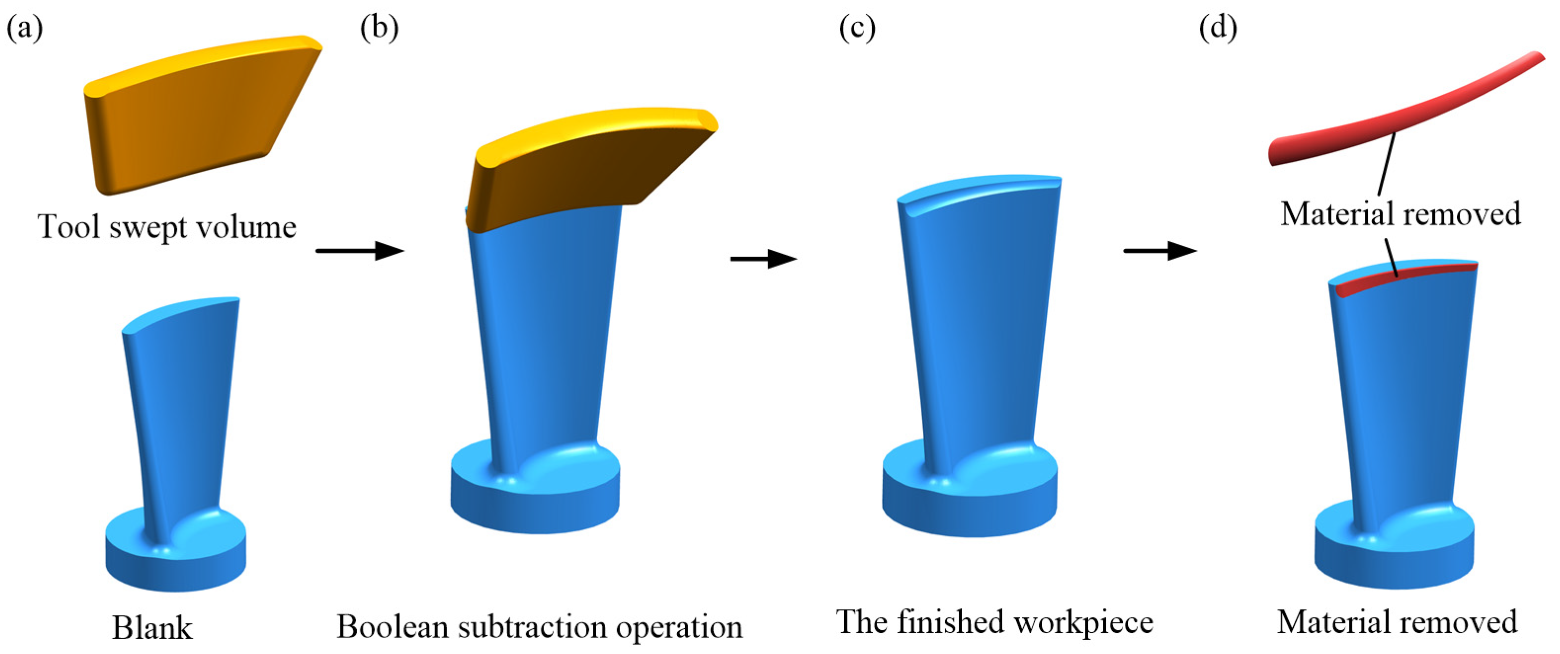
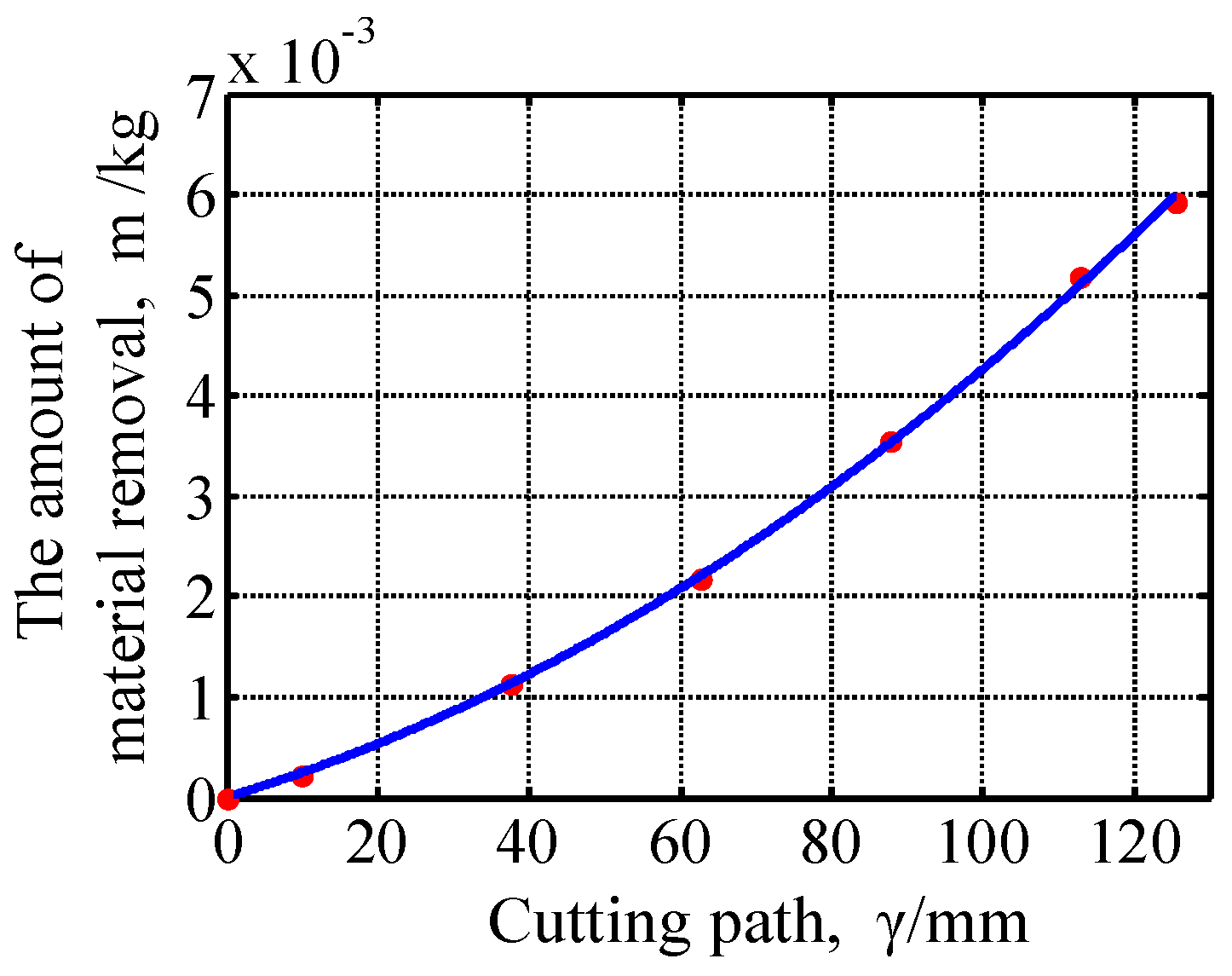
where m_RM is the total amount of material removal during the cutting process. The subscripts ‘n’ and ‘0′ indicate the final machined workpiece and initial un-machined workpiece, respectively. m_i,n, m_i,0, c_i,n, c_i,0, k_i,n, k_i,0 are the mass, stiffness, and damping of the final machined workpiece and initial un-machined workpiece, respectively. δm_i is a mass that is removed corresponding to the ith structure modification, which can be obtained through the following procedure. The material removed during the cutting process is acquired through Figure 4, and the relationship between the material removed and the n cutting steps is presented in Figure 6. It can be known from Figure 6 that the mass of material removed in ith cutting step is expressed as

$$\delta m_i=m\left(\mu \right)-m\left(\nu \right)$$

(12)

where μ and ν indicate the starting and endpoints of the ith tool path segment, respectively. It is emphasized that δm_i is dependent on the cutting path and is generally a function of the tool position (or time), which is different from the case presented in Ref. [33] (where δm_i is constant). Here, δm_i is extracted through the CL files generated using the CAD program package.

To identify the corrected FRFs of the workpiece during the cutting process, SDMM-EM proposed that the FRF of the workpiece is presented in excitation coordinate, response coordinate, and the modified structural positional co-ordinates, in addition to the side effects caused by the removed material at active coordinates are removed [33]. For the ith structural modifications along the tool path at the position coordinates γ, the frequency response function $h_{\alpha \beta ,i}^{\gamma }$ at response point coordinates of α, excitation point coordinates of β can be express as

$$h_{\alpha \beta ,i}^{\gamma }=\frac{h_{\alpha \beta ,i-1}^{\gamma }+\left(-{\omega }^2\Delta m_i+j\omega \Delta c_i+\Delta k_i\right)\left(h_{\gamma \gamma ,i-1}^{\gamma }{h}_{\alpha \beta ,i-1}^{\gamma }-h_{\alpha \gamma ,i-1}^{\gamma }{h}_{\gamma \beta ,i-1}^{\gamma }\right)}{1+\left(-{\omega }^2\Delta m_i+j\omega \Delta c_i+\Delta k_i\right)h_{\gamma \gamma ,i-1}^{\gamma }}$$

(13)

where $h_{\alpha \beta ,i-1}^{\gamma }$ is the FRF before the ith structure modification (or after the (i − 1)th modification), and $h_{\alpha \beta ,i}^{\gamma }$ is the FRF after the ith structure modification (or before the (i + 1)th modification). Equation (13) is the general form to calculate the frequency response after the structure modification. Since the cutting process is divided into n cutting steps along the cutting tool path, γ is the center position coordinates of the cutting steps before and after structure modification. Therefore, the relationship between the position coordinate γ and the cutting step i can be expressed as

$$\gamma =f(i)$$

(14)

The specific function expression in Equation (14) is related to the number of cutting steps. Therefore, for each modification, n FRFs corresponding to different positional coordinates γ can be obtained through Equation (13) with fixed the excitation coordinate and response coordinate.

According to the assumption presented in SDMM, the direct FRF (α = β) corresponding to the ith position before the ith modification is used in Equation (1) to analyze the cutting stability. Hence, Equation (13) can be expressed as

$$h_{rr,i}=\frac{h_{rr,i-1}+\left(-{\omega }^2\Delta m_i+j\omega \Delta c_i+\Delta k_i\right)\left(h_{\gamma \gamma ,i-1}{h}_{rr,i-1}-h_{r\gamma ,i-1}{h}_{\gamma r,i-1}\right)}{1+\left(-{\omega }^2\Delta m_i+j\omega \Delta c_i+\Delta k_i\right)h_{\gamma \gamma ,i-1}}.$$

(15)

In Equation (15), h_rt,i (r = 1, 2, …, n; t = 1, 2, …, n) is instead of $h_{\alpha \beta ,i}^{f(i)}$. The structural modifications positional coordinates after the ith structure modification is f(i), thus the cutting step corresponding to the excitation point is t (i.e., β = f(t)), the cutting step corresponding to the response point is r (i.e., α = f(r)). Equation (15) indicates how to determine the direct FRF at point α (or r, α = β, and r = t) using the known FRFs obtained for (i − 1)th modification, when the ith modification (γ = f(i)) is performed. When the excitation point, the response point, and the structural modification point are in the same positions, that is, α = β = γ (or r = t = i), as shown in Figure 5b,c, then Equation (15) can be expressed as

$$h_{ii,i}=\frac{h_{ii,i-1}}{1+\left(-{\omega }^2\Delta m_i+j\omega \Delta c_i+\Delta k_i\right)h_{ii,i-1}}.$$

(16)

By Equation (16), the frequency response function at the structure modification position $\gamma$ (the ith cutting step) can be obtained. Correspondingly, the original frequency response function after structure modification can be obtained easily, provided that we know the original frequency response function before structure modification and the change of modal mass, modal damping, and modal stiffness of this structure modification.

3.2. Implementation Procedure

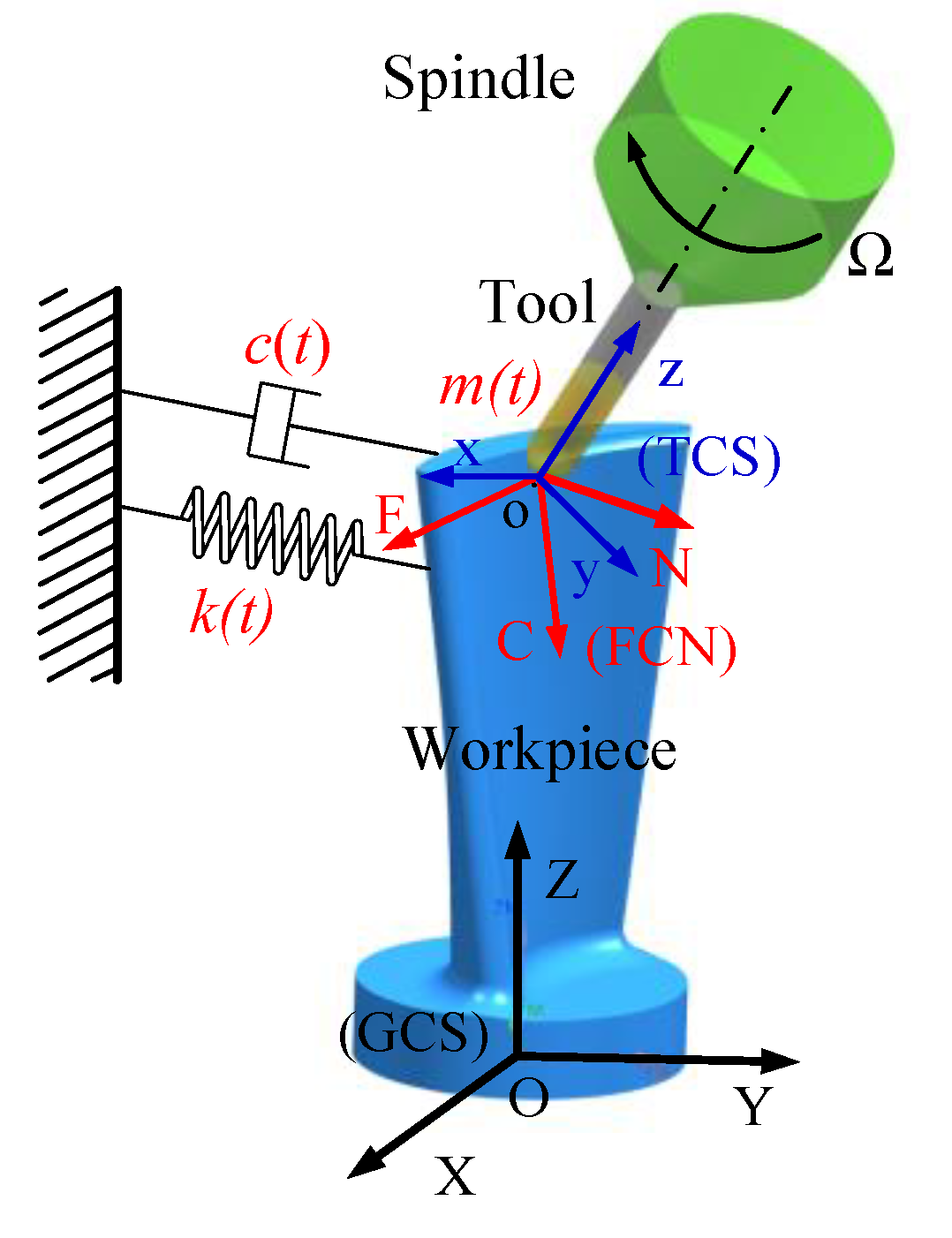
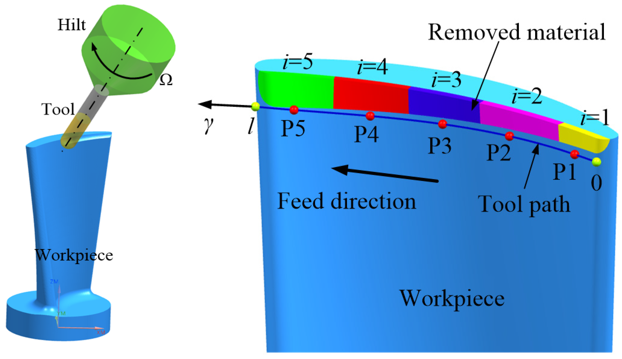
In the multi-axis milling process of thin-walled parts, as shown in Figure 1, the coordinates of the excitation point, the response point, and the structural change point are the same (α = β = γ). The direction of excitation and response are in the normal direction along the workpiece surface, which is perpendicular to the direction of the tool path. Due to the multi-axis milling, the path is divided into n cutting steps; the coordinates and the original frequency response function of different cutting steps are different. The main work here is to study the dynamic characteristics of the original function with the change of the cutting path.

The FEM or experimental modal analysis (EMA) can be used to obtain the original frequency response function and the cross-point frequency response function at the n-cutting step midpoint coordinates of the initial un-machined workpiece (i = 0) and final machined workpiece (i = n). According to the obtained frequency response function, by Equation (11), the change amount of modal mass, modal damping, and modal stiffness can be obtained in each structural modification process after the ith (i = 0, 1, 2, …, n) structure modification. By Equation (16), the frequency response function between any two points can be obtained. The flowchart for the calculation of the frequency response function at the original position point of each cutting step is shown in Figure 7. In the figure, the black solid arrow represents the material removal, which is the forward method; the red solid arrow represents the addition of material, which is the reverse method. Both methods generate the same results. The specific steps and the verification process of both methods are described as follows:

Step 1: Divide the cutting process into n cutting steps (or cutting positions) along the cutting tool path, γ = f(i) is expressed as the position coordinates of the ith cutting step (i = 0, 1, 2, …, n). The β = f(t) (t = 1, 2, …, n) is defined as excitation point coordinates and the α = f(r) (r = 1, 2, …, n) is defined as the response point coordinate along the tool path. The above formula indicates that the excitation point coordinate corresponds to the t cutting step, and the response point coordinate corresponds to the r cutting step;

Step 2: For i = 0, that is the initial system with no structural modification at each cutting position, modal analyses (using EMA or FEM) are conducted to obtain the origin-point and the cross-point FRFs ${\overline{h}}_{rt,0}$;

Step 3: For i = n, that is the final system after the ith structure modification at each cutting position, modal analyses (using EMA or FEM) are conducted to obtain the origin-point and the cross-point FRFs ${\overline{h}}_{rt,n}$;

Step 4: Eliminate the accelerometer mass loading effect by Equation (15), obtain the corrected FRFs of initial and final system structure h_rt,0, h_tr,n if the modal parameters are obtained by the EMA method in steps 2 and 3. This step is not necessary if the modal parameters are obtained by FEM;

Step 5: Extract the modal mass (m_r,0, m_r,n), modal damping(c_r,0, c_r,n), and modal stiffness (k_r,0, k_r,n) parameters from the FRFs, h_rt,0, h_tr,n. Using Equation (11) calculate the Δm_r, Δc_r, and Δk_r. It is worth noting that the subscript r here and the subscript i in Equation (11) have the same meaning, that is, Δm_i = Δm_r, Δc_i = Δc_r, Δk_i = Δk_r;

Step 6: For i = 1, 2, …, n−1, calculate the origin-point and the cross-point FRFs at the midpoint position of each cutting step using Equation (15);

Step 7: For i = 1, 2, …, n, calculate the original frequency response function h_ii,i-1 from Step 6 at the midpoint of each cutting step, and the modal parameters are obtained.

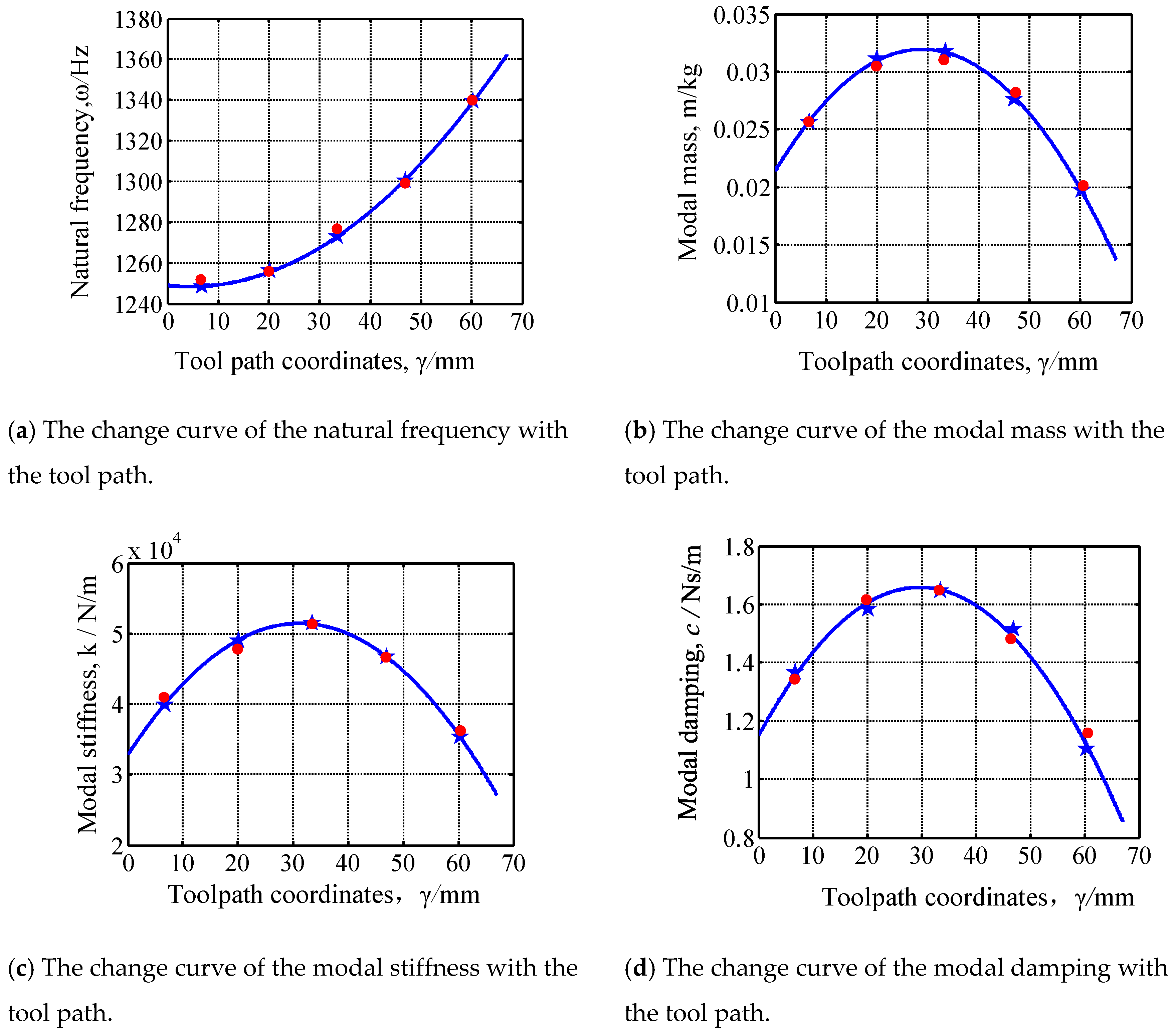
Finally, the time-varying dynamic characteristics of the thin-walled workpiece with a complex curved surface and variable thickness can be obtained in the milling process after the FRFs of different tool positions for original and final structures are provided. After the n frequency response functions at the position of the required machining process are obtained, and extracting the dynamic characteristics of the n frequency response functions, the curves of the dynamic characteristics with the change of cutting path are drawn. Thereby, we can conduct the stability prediction, draw the stability limit diagram, optimize the processing parameters, and improve the processing efficiency according to the dynamic characteristic curves.

4. Experimental Setup and Procedure

To verify the accuracy of the method aimed at obtaining the instantaneous dynamic characteristics in the multi-axis milling process using the extended Sherman–Morrison–Woodbury formula, an experimental study is conducted. The experiment mainly consists of two parts: the modal experiment and the cutting experiment. The former mainly aims at obtaining the original and the cross-point frequency response function at different positions of the workpiece before and after machining, while the latter mainly aims at getting the workpiece after machining and conducting the modal experiment. It worth noting that, in the cutting experiment, whether one measures the cutting force of the workpiece during machining, or one measures the vibration of the workpiece with the laser displacement sensor during machining, neither is relevant to the instantaneous dynamic characteristics of the workpiece under discussion in this section, and the measurement is mainly used for other analysis.

The devices used in the cutting and modal experiments are shown in Figure 8. The machine used in the process of the cutting experiments is a high-speed milling machining center VMC0540d with a maximum speed of 30,000 rpm, maximum power of 42 kW, and maximum torque of 22 N•m. The cutter used in the experiment is a cemented carbide end milling tool with a diameter of 20 mm, helix angle of 30°, overhang length of 67 mm, and tool tooth number 3. Compared with the workpiece to be machined, the tool stiffness is much larger than that of the workpiece, so that the milling cutter can be assumed to have a rigid structure, and the workpiece is considered to be flexible. In the experiment, the workpiece material is aluminum alloy 7050, and physical parameters of the workpiece are shown in

Table 1. Geometric and physical parameters of the workpiece.

Workpiece Materials	Geometric Dimensions (mm)			Density (kg/m3)	Elastic Modulus (GPa)	Poisson Ratio
	Long	Wide	Thick
Al 7075	67	64	4	2.82 × 103	70.3	0.33

. Fixed with clamps, the overhang is 50 mm and works along the longitudinal direction of the workpiece, as shown in Figure 8a. In the experiment, the feed per tooth is 0.05 mm, and the radial cutting depth linearly varies from 0 mm to 2 mm. When cutting along the length direction of the completed workpiece, the radial cutting depth is changed to 2 mm.

The workpiece is divided into five (n = 5) cutting steps along the machining path. The length of each cutting step is 13.4 mm, and the midpoint of each cutting step is taken as the excitation point and the response point of the modal experiment. The dynamic characteristics of the whole length of the cutting step are substituted by the original frequency response function at the midpoint of each cutting step. The position coordinates of the midpoint of the five cutting steps are P1: 6.7 mm, P2: 20.1 mm, P3: 33.5 mm, P4: 46.9 mm, and P5: 60.3 mm. The original and cross-point frequency response function at the midpoint of five steps before and after the cutting process was measured, respectively. The modal parameters are extracted from the original frequency response function.

To verify the accuracy of the semi-discrete method and to obtain the stability limit diagram of delay differential equations with time-varying parameters of thin-walled parts with a complex curved surface and variable thickness during the multi-axis milling process, an experimental study was conducted. In the experiment, different machining conditions were set up, see

Table 2. Cutting conditions.

Condition Number	Rotating Speed (rpm)	Axial Depth (mm)	Radial Depth (mm)
C1	5000	8	0–2
C2	10,000	8	0–2
C3	16,000	8	0–2
C4	5000	12	0–2
C5	10,000	12	0–2
C6	16,000	12	0–2

, and the surface quality of the machined workpiece (presented in the following section) was employed to estimate the stability of the cutting process. Finally, the results obtained from different processing conditions were compared with the stability limit diagram. The experimental devices used in this section are shown in Figure 8.

5. Result Analysis

The results of the dynamic characteristic experiment are mainly used as the initial input of the calculation of the frequency response function matrix of the multi-axis milling process. Using the extended Sherman–Morrison–Woodbury formula, one will eventually get the original frequency response function. Then, the modal parameters are extracted from the original frequency response function, and the variation curves of the modal parameters with the change of the machining path are drawn. To verify the accuracy of the obtained results, a finite element model is built according to the division of the cutting steps, the modal analysis of the finite element model is conducted, and the modal parameters are obtained. Then the results of finite element analysis are compared with the results obtained by the extended Sherman–Morrison–Woodbury formula. The finite element analysis results are in good agreement with the prediction using the extended Sherman–Morrison–Woodbury formula. The results show that the proposed method is of high accuracy. Besides, the machining of blades as a typical case of multi-axis milling of a thin-walled part with a complex curved surface is studied. The research of the multi-axis milling process is one of the tops of the blade during the semi-finishing machining process. Using the proposed method, we obtained the variation of natural frequency, modal mass, modal stiffness, and modal damping of the blade with the cutting path in the multi-axis milling process. The effectiveness of this method is validated.

5.1. FRF Analysis

In the machining, the amount of material removal by each cutting step and the amount of the total material removal can be obtained from Figure 9.

In Figure 9, the relationship between the amount of material removal m(γ) and the cutting path γ can be expressed as

$$m(\gamma )=5.05\times {10}^{-7}{\gamma }^2.$$

(17)

The original frequency response functions at the midpoint of each cutting step before and after machining are obtained from the modal experiment, excluding the influence of the acceleration sensor on the frequency response function, so the modal parameters of each cutting step before and after machining are obtained, as shown in

Table 3. Modal parameters at different locations before and after machining.

	Modal Parameters	ωi,0 (Hz)	ωi,n (Hz)	mi,0 (kg)	mi,n (kg)	ci,0 (Ns/m)	ci,n (Ns/m)	ki,0 (N/m)	ki,n (N/m)
Position Coordinates
P1		1253	1359	0.0240	0.0192	1.42	0.94	37,747.2	35,408.3
P2		1253	1359	0.0312	0.0248	1.87	1.34	49,024.4	45,880.0
P3		1253	1359	0.0334	0.0261	2.04	1.49	52,424.6	48,185.8
P4		1253	1359	0.0312	0.0236	1.87	1.34	49,024.4	43,546.4
P5		1253	1359	0.0240	0.0178	1.42	1.03	37,747.2	32,841.8

. According to the data in the table, the modal mass, modal damping, and modal stiffness of each cutting step can be obtained, as shown in Figure 10 by the Equation (11).

As can be seen from Table 3, the natural frequency at the midpoint of the each cutting step before and after the machining remains constant, before machining the natural frequency is 1253 Hz, the after machining natural frequency is 1359 Hz. This shows that the structure of the workpiece is unchanged. From the modal stiffness values at the midpoint of each cutting step before machining, it can be found that the modal stiffness value (37,747.2 N/m) on both sides of the workpiece is less than the modal stiffness values (52,424.6 N/m) in the middle position. It is well explained that the deformation of the workpiece on both sides is greater than the deformation of the workpiece in the middle position of the phenomenon. Comparing the value of the stiffness of the same position before and after machining, it can be found that the greater the amount of material removal there is (the workpiece becomes thinner), the more the modal stiffness of the workpiece decreases. At point P₁, the modal stiffness value is 37,747.2 N/m before machining, and the value is 35,408.3 N/m after machining, with a stiffness decrease of 2338.9 N/m. At point P₅, the modal stiffness value is 37,747.2 N/m before machining, the modal stiffness value is 32841.8 N/m after machining, and the amount of change is 4905.4 N/m. In addition, the variation of the modal mass values and the modal damping values before and after machining is basically the same along the machining path. In other words, the modal mass values and the modal damping values at the midpoint of the workpiece have reached the maximum and gradually decrease to both sides.

After obtaining the frequency response function matrix of the machining, depending on the application of extended Sherman–Morrison–Woodbury formula presented in previous, we calculated the original frequency response function at the midpoint of each cutting step in the process and extracted the modal parameters. Thereby, to verify the accuracy of the formula, the finite element model of different cutting steps was established, the finite element analysis was conducted, and the analysis results were post-processed to extract the dynamic characteristic parameters. The dynamic characteristic parameters of each cutting step in the process obtained by both methods were plotted for each dynamic parameter changing with the cutting path, and the final results are shown in Figure 10. In the figure, the red solid circles represent the results of the finite element analysis, the blue five-pointed stars represent the results predicted by the extended Sherman–Morrison–Woodbury formula, and the blue curves are the results that were fitted by the least square method according to the blue five-pointed star.

According to the prediction by the extended Sherman–Morrison–Woodbury formula, the results are fitted by the least square method, and the relationship of the dynamic characteristic parameters of the cutting process with the tool path is shown in

Table 4. The relationship of dynamic characteristics with the change of the processing path.

Modal Parameters	Expressions	R2	Diagrams
Natural frequency, Hz	$\omega (\gamma )=0.02924{\gamma }^2-0.2687\gamma +1249$	0.9999	Figure 10a
Modal mass, kg	$m(\gamma )=-1.261\times {10}^{-5}{\gamma }^2+7.307\times {10}^{-4}\gamma +2.136\times {10}^{-2}$	0.9985	Figure 10b
Modal stiffness, N/m	$k(\gamma )=-19.11{\gamma }^2+1195\gamma +32780$	0.9998	Figure 10c
Modal damping, N-s/m	$c(\gamma )=-5.776\times {10}^{-4}{\gamma }^2+3.428\times {10}^{-2}\gamma +1.15$	0.9921	Figure 10d

.

Figure 10a indicates that, initially, the amount of material removal was less, and the natural frequency of the workpiece along the machining path increased slowly, with the increase in the amount of material removal, the natural frequency of the workpiece increased significantly. The more material is removed, the greater the natural frequency of the workpiece is changed. Namely, in the thin-walled parts of the multi-axis milling process with a large amount of cutting, the influence of material removal on the dynamic characteristics of the workpiece cannot be ignored. From Figure 10b,c, it can be seen that in the process of machining, the modal mass, the modal stiffness, and the modal damping variation trends are consistent, they first increase and then decrease, and the whole trend is a parabolic shape. From the graph, we can find that the symmetry axis of the three parabolas is not in the midpoint position of the cutting tool path, which is mainly caused by material removal. In addition, comparing the predicted results by finite element analysis and the application of extended Sherman–Morrison–Woodbury formula, we find that the results of the finite element analysis simulation and the results predicted by applying the Sherman–Morrison–Woodbury formula have a high consistency; both the size and change tendency are consistent. In other words, the method of using the extended Sherman–Morrison–Woodbury formula to obtain the dynamic characteristic of the workpiece during the machining process is accurate. When the variation of the dynamic characteristic of the cutting process with the tool path has been obtained, we can predict the machining process stability, optimize the cutting parameters, and improve the processing efficiency.

5.2. Case Study: Multi-Axis Milling of Aero-Engine Blade

The experiments have proven that the accuracy of the dynamic characteristics of the workpiece is obtained by using the extended Sherman–Morrison–Woodbury formula. Next, the method is applied to the typical multi-axis milling process. We used the FEM to obtain the initial dynamic characteristics of the workpiece, and then used the proposed method to obtain the dynamic characteristics of the workpiece during the machining process.

The model of the multi-axis milling time-varying parameter system of the blade is shown in Figure 11. The dynamic characteristic variation of the workpiece when the top of the blade material is removed during the semi-finishing process was simulated. The blade is a typical multi-axis milling molding part, the material is Al7050, the height is 213.3 mm, the blank margin is 3 mm, the blank thickness is 8–20 mm, the middle part of the blade is thicker, the thickness is 20 mm, the two sides are thinner, the thickness is 8 mm. In the machining process, the tool used is a carbide ball-end cutter with a diameter of 20 mm and an 82 mm overhang. Due to the workpiece overhang being longer, the rigidity is small, so the dynamic characteristics of the workpiece have a significant impact on the processing stability of the multi-axis milling system.

The multi-axis milling semi-finishing at the top of the blade of the tool path can be obtained with CAM software. The total length of the tool path was 125.48 mm. Along the path and the whole process was divided into five cutting steps, the five cutting steps at the midpoint of the position coordinates were P1: 10 mm, P2: 37.65 mm, P3: 62.74 mm, P4: 87.84 mm, P5: 60.3 mm, as shown in Figure 11.

In the machining, the relationship between the amount of material removal and the tool path is shown in Figure 12. As can be seen from the figure, the amount of material removal along the tool path is a nonlinear change. Because of the complex spatial characteristics of the tool movement, so in the traditional analytic method it is difficult to obtain the variation of material removal.

The variation of the amount of material removal m(γ) with the cutting path γ in this picture can be expressed as

$$m(\gamma )=2\times {10}^{-7}{\gamma }^2+2.26\times {10}^{-5}\gamma , R^2=0.9997.$$

(18)

The original and the cross-point frequency response function of the midpoint of five cutting steps before and after machining were obtained using the FEM. We calculated the variation amount of the modal mass, modal stiffness, and modal damping in each structural modification, and then took the obtained calculation results as the initial condition, using the proposed method to extract the modal parameters, the results are shown in Figure 13.

The blue stars represent the dynamic characteristics of the different positions predicted by using the extended Sherman–Morrison–Woodbury formula. On the basis of the results, the relationship of the dynamic characteristic parameters of the cutting process with the tool path was obtained by the least square method, as shown in

Table 5. The relationship of dynamic characteristics with the change of the processing path.

Modal Parameters	Expressions	R2	Diagrams
Natural frequency, Hz	$\begin{array}{l}\omega (\gamma )=-8.611\times {10}^{-6}{\gamma }^3+1.752\times {10}^{-3}{\gamma }^2\\ -1.261\times {10}^{-2}\gamma +1022\end{array}$	0.9835	Figure 13a
Modal mass, kg	$\begin{array}{l}m(\gamma )=-2.434\times {10}^{-6}{\gamma }^2+3.184\times {10}^{-4}\gamma \\ +2.208\times {10}^{-2}\end{array}$	0.9996	Figure 13b
Modal stiffness, N/m	$k(\gamma )=-2.548{\gamma }^2+338.2\gamma +22960$	0.9999	Figure 13c
Modal damping, N-s/m	$\begin{array}{l}c(\gamma )=-7.803\times {10}^{-4}{\gamma }^2+9.828\times {10}^{-2}\gamma \\ +7.326\times {10}^{-1}\end{array}$	0.9856	Figure 13d

.

Figure 13 indicates that in the complicated blade multi-axis milling process, various forms of the tool movement and the material removal effect directly lead to the change of the dynamic characteristics of the blade (such as natural frequency, modal mass, modal stiffness, modal damping) when the cutting path is more complicated. Meanwhile, the natural frequency increased with the cutting path, the other three first increased and then decreased. The variation trend was consistent with the previous experimental results. Therefore, the existing cutting strategies, cutting process and cutting parameters are conservative, and the processing efficiency is low. The stability of the multi-axis milling can be predicted when the dynamic characteristic variation of the workpiece is obtained. Under the premise of a stable machining process, increasing the cutting parameters is beneficial to shorten the production cycle and improve the production efficiency.

According to the corrected dynamic characteristics (see Figure 10) of the workpiece system with respect to cutting positions along machining direction, the 3D-SLD of the thin-walled workpiece milling was evaluated for different tool positions and spindle speeds by the semi-discrete method, as shown in Figure 14. Figure 14a is a 3D-SLD. The three coordinate axes represent the spindle speed, tool position, and axial depth, respectively. The combinations of the cutting parameters in the zones of the curved lines below are stable cases, and those in the zones of the curved lines above are unstable cases. At different locations of the workpiece in the machining process, the processing parameters can, according to Figure 14a, select the best combination of spindle speed and axial depth of the cut, making the whole cutting process remain in a stable condition. Figure 14b presents a new graphic chart only determined by the “tool position” axis and “axial cutting depth” axis. Which is easy to apply to optimize the cutting parameters such as the spindle speed and axial cutting depth. Without a loss of generality, six cutting conditions, as shown in Table 2, are implemented, in which three different spindle speeds (5000 rpm, 10,000 rpm and 16,000 rpm) are selected under two different axial cutting depths (a_p = 8 mm: pink dotted line; a_p = 12 mm: purple dotted line). The photographs of machined workpiece under six cutting conditions and its partial enlargement diagram are included in

Table 6. Machined workpiece under six cutting conditions.

No.	Finished Surface	Partial Enlargement Diagram of Finished Surface
1	Unstable after the first stable
2	Both sides are unstable and the middle is stable.
3	Unstable after the first stable
4	Has been unstable
5	Has been unstable
6	Both sides are unstable and the middle is stable.

.

From Figure 14, it has been observed that the variation of the dynamic characteristics of the thin-walled part with a complex curved surface and variable thickness introduces a change of the axial cutting depth SLD with respect to the spindle speed. If it changes a lot, it would be possible that a few stable cases exist. For example, under condition 2, the speed is 10,000 rpm (green solid line), a_p = 8 mm (pink dotted line). Similar to the illustrations presented above, the part of the green solid line below the pink dotted line are the unstable zones, and the part of the green solid line above the pink dotted line are the stable zones. In other words, in condition 2, the workpiece experienced unstable cutting, stable cutting, and unstable cutting in a total of three processes. It should be underlined that, Figure 14 shows the stability limit diagram results in the cutting conditions with a_p = 8 mm and 12 mm, because the dynamic characteristics used are assessed in these cutting conditions, as described in the previous part.

To verify the accuracy of the dynamic stability limit diagram, as above, the photographs of the workpiece machined surface under six cutting conditions were obtained, as shown in Table 6. In Table 6, the regions denoted by the labels a–n are in accordance with those in Figure 14b. By comparing the stability limit diagram of Figure 14b with Table 6 in different cutting conditions, good agreement was found by comparing the stability limit diagram obtained through the extended numerical integrated method and experiment with the different working conditions, which indicates that the stability limit diagram that has been obtained is correct. That is to say, we can use the stability limit diagram that has been obtained to select the processing parameters so that the cutting process is carried out in a stable region.

6. Conclusions

The main results of the research on the machining system and the stability of the machining system of thin-walled parts with a complex curved surface and variable thickness during multi-axis milling can be summarized as follows: an improved structural dynamic modification method with variable mass was proposed to identify the instantaneous variation of natural frequency, modal mass, modal stiffness, and modal damping of a typical complex curved surface thin-walled part (the machining of blades). It is not necessary to re-build and remesh the FEM model at each cutting step, and it can be implemented automatically through the program, so that the processing efficiency improves greatly. Good agreement was found by comparing the stability limit diagram obtained through the extended numerical integrated method and the experiment with the different working conditions.

This paper focuses on the study of the cutting force, dynamic characteristic parameters, and the delay differential equations of time-varying parameters related to the instability characteristics of multi-axis milling of thin-walled parts with varying thickness of the complex curved surface are studied. However, the instability characteristics of multi-axis milling involve a number of affecting factors. It is also an urgent problem to optimize the parameters of the spindle speed, feed rate, tool inclination, tool path, axial cutting depth, and radial cutting depth automatically by combining the stability analysis results of the multi-axis milling of thin-walled parts with the numerical control system.

References

1. Altintas, Y.; Engin, S. Generalized modeling of mechanics and dynamics of milling cutters. Cirp. Ann. Manuf. Technol. 2001, 50, 25–30. [Google Scholar] [CrossRef]
2. Altintas, Y.; Budak, E. Analytical prediction of stability lobes in milling. CIRP Ann. Manuf. Technol. 1995, 44, 357–362. [Google Scholar] [CrossRef]
3. Ozturk, E.; Budak, E. Modelling of 5 axis milling forces. Proc. CIRP 2005, 319–332. [Google Scholar]
4. Tsai, C.L.; Liao, Y.S. Prediction of cutting forces in ball end milling by means of geometric analysis. Int. J. Mater. Process. Technol. 2008, 205, 24–33. [Google Scholar] [CrossRef]
5. Saffar, R.J.; Razfar, M.R.; Zarei, O. Simulation of three dimension cutting force and tool deflection in the end milling operation based on finite element method. Simul. Modell. Pract. Theory 2008, 16, 1677–1688. [Google Scholar] [CrossRef]
6. Sun, Y.; Guo, Q. Numerical simulation and prediction of cutting forces in multi axis milling processes with cutter run out. Int. J. Mach. Tools Manuf. 2011, 51, 806–815. [Google Scholar] [CrossRef]
7. Tunc, L.T.; Ozkirimli, O.; Budak, E. Generalized cutting force model in multiaxis milling using a new engagement boundary determination approach. Int. J. Adv. Manuf. Technol. 2015, 77, 341–355. [Google Scholar]
8. Ozkirimli, O.; Tunc, L.T.; Budak, E. Generalized model for dynamics and stability of multi-axis milling with complex tool geometries. Int. J. Mater. Process. Technol. 2016, 238, 446–458. [Google Scholar] [CrossRef]
9. Song, Q.; Liu, Z.; Ju, G.; Wan, Y. A generalized cutting force model for five-axis milling processes. Proc. I Mech. E Part B J. Eng. Manuf. 2019, 233, 3–17. [Google Scholar] [CrossRef]
10. Liu, C.; Li, Y.; Jiang, X.; Shao, W. Five-axis flank milling tool path generation with curvature continuity and smooth cutting force for pockets. Chin. J. Aeronaut. 2020, 33, 730–739. [Google Scholar] [CrossRef]
11. Yue, C.; Gao, H.; Liu, X.; Liang, S.Y.; Wang, L. A review of chatter vibration research in milling. Chin. J. Aeronaut. 2019, 32, 215–242. [Google Scholar] [CrossRef]
12. Budak, E.; Altintas, Y. Analytical prediction of chatter stability in milling-partⅡ: General formulation. J. Dyn. Syst. T ASME 1998, 120, 22–30. [Google Scholar] [CrossRef]
13. Altintas, Y. Manufacturing Automation: Metal Cutting Mechanics, Machine Tool Vibration, and CNC Design, 2nd ed.; Cambridge University Press: New York, NY, USA, 2012. [Google Scholar]
14. Totis, G.; Albertelli, P.; Sortino, M.; Monno, M. Efficient evaluation of process stability in milling with spindle speed variation by using the Chebyshev collocation method. J. Sound Vib. 2014, 333, 646–668. [Google Scholar] [CrossRef]
15. Ozoegwu, C.G. Least squares approximated stability boundaries of milling process. Int. J. Mach. Tools Manuf. 2014, 79, 24–30. [Google Scholar] [CrossRef]
16. Bravo, U.; Altuzarra, O.; De Lacalle, L.N.L. Stability limits of milling considering the flexibility of the workpiece and the machine. Int. J. Mach. Tools Manuf. 2005, 45, 1669–1680. [Google Scholar] [CrossRef]
17. Wan, M.; Ma, Y.C.; Zhang, W.H.; Yang, Y. Study on the construction mechanism of stability lobes in milling process with multiple modes. Int. J. Adv. Manuf. Technol. 2015, 79, 589–603. [Google Scholar] [CrossRef]
18. Mane, I.; Gagnol, V.; Bouzgarrou, B.C. Stability based spindle speed control during flexible workpiece high speed milling. Int. J. Mach. Tools Manuf. 2008, 48, 184–194. [Google Scholar] [CrossRef]
19. Tang, A.; Liu, Z. Three dimensional stability lobe and maximum material removal rate in end milling of thin walled plate. Int. J. Adv. Manuf. Technol. 2009, 43, 33–39. [Google Scholar] [CrossRef]
20. Kolluru, K.; Axinte, D. Novel ancillary device for minimising machining vibrations in thin walled assemblies. Int. J. Mach. Tools Manuf. 2014, 85, 79–86. [Google Scholar] [CrossRef]
21. Guo, M.; Wei, Z.; Wang, M.; Li, S.; Wang, J.; Liu, S. Modal parameter identification of general cutter based on mill ing stability theory. J. Intell. Manuf. 2020. online. [Google Scholar]
22. Thevenot, V.; Arnaud, L.; Dessein, D.; Cazenave, L.G. Integration of dynamic behavior variations in the stability lobes method: 3D lobes construction and application to thin-walled structure milling. Int. J. Adv. Manuf. Technol. 2006, 27, 638–644. [Google Scholar] [CrossRef] [Green Version]
23. Thevenot, V.; Arnaud, L.; Dessein, G.; Cazenave, L.G. Influence of material removal on the dynamic behavior of thin-walled structures in peripheral milling. Mach. Sci. Technol. 2006, 10, 275–287. [Google Scholar] [CrossRef]
24. Campa, F.J.; Lopezde-Lacalle, L.N.; Celaya, A. Chatter avoidance in the milling of thin floors with bull-nose end mills: Model and stability diagrams. Int. J. Mach. Tools Manuf. 2011, 51, 43–53. [Google Scholar] [CrossRef] [Green Version]
25. Biermann, D.; Kersting, P.; Surmann, T. A general approach to simulating workpiece vibrations during five-axis milling of turbine blades. CIRP Ann. Manuf. Technol. 2010, 59, 125–128. [Google Scholar] [CrossRef]
26. Brecher, C.; Altstädter, H.; Daniels, M. Axis position dependent dynamics of multi-axis milling machines. Proc. CIRP 2015, 31, 508–514. [Google Scholar] [CrossRef] [Green Version]
27. Zhou, X.; Zhang, D.; Luo, M.; Wu, B. Chatter stability prediction in four-axis milling of aero-engine casings with bull-nose end milling. Chin. J. Aeronaut. 2015, 28, 1766–1773. [Google Scholar] [CrossRef] [Green Version]
28. Shi, J.; Song, Q.; Liu, Z.; Ai, X. A novel stability prediction approach for thin-walled component milling consider ing material removing process. Chin. J. Aeronaut. 2017, 30, 1789–1798. [Google Scholar] [CrossRef]
29. Song, Q.; Wan, Y.; Ai, X. Stability prediction during thin walled workpiece high speed milling. Adv. Mater. Res. 2009, 69, 428–432. [Google Scholar] [CrossRef]
30. Shao, W.; Li, Y.; Liu, C. Tool path generation method for five-axis flank milling of corner by considering dynamic characteristics of machine tool. Proc. Cirp. 2016, 56, 155–160. [Google Scholar] [CrossRef] [Green Version]
31. Yan, Q.; Luo, M.; Tang, K. Multi-axis variable depth-of-cut machining of thin-walled workpieces based on the workpiece deflection constraint. Comput. Aided Des. 2018, 100, 14–29. [Google Scholar] [CrossRef]
32. Biermann, D.; Surmann, T.; Kersting, P. Oscillator-based approach for modelling process dynamics in NC milling with position- and time- dependent modal parameters. Prod. Eng. Res. Develop. 2013, 7, 417–422. [Google Scholar] [CrossRef]
33. Song, Q.; Liu, Z.; Wan, Y.; Ju, G.; Shi, J. Application of Sherman-Morrison-Woodbury formulas in instantaneous dy-namic of peripheral milling for thin-walled component. Int. J. Mech. Sci. 2015, 96, 79–90. [Google Scholar] [CrossRef]
34. Dun, Y.; Zhu, L.; Wang, S.Y. Multi-modal method for chatter stability prediction and control in milling of thin-walled workpiece. Appl. Math. Model. 2020, 80, 602–624. [Google Scholar] [CrossRef]
35. Shi, J.; Gao, J.; Song, Q.; Liu, Z.; Wan, Y. Dynamic deformation of thin-walled plate with variable thickness under moving milling force. Proc. CIRP 2017, 58, 311–316. [Google Scholar] [CrossRef]
36. Wu, Q.; Zhang, Y.; Zhang, H. Dynamic characteristic analysis and experiment for integral impeller based on cyclic symmetry analysis method. Chin. J. Aeronaut. 2012, 25, 804–810. [Google Scholar] [CrossRef] [Green Version]
37. Nikolaev, S.; Kiselev, I.; Kuts, V.; Voronov, S. Optimal milling modes identification of a jet-engine blade using time-domain technique. Int. J. Adv. Manuf. Technol. 2020, 107, 1983–1992. [Google Scholar] [CrossRef]
38. Tuysuz, O.; Altintas, Y. Frequency Domain Updating of Thin-Walled Workpiece Dynamics Using Reduced Order Substructuring Method in Machining. Asme J. Manuf. Sci. Eng. 2017, 7, 139. [Google Scholar] [CrossRef]
39. Budak, E.; Tun, L.T.; Alan, S. Prediction of workpiece dynamics and its effects on chatter stability in milling. CIRP Ann. Manuf. Technol. 2012, 61, 339–342. [Google Scholar] [CrossRef]
40. Song, Q.; Ai, X.; Tang, W. Prediction of simultaneous dynamic stability limit of time–variable parameters system in thin-walled workpiece high-speed milling processes. Int. J. Adv. Manuf. Technol. 2011, 55, 883–889. [Google Scholar] [CrossRef]
41. Ju, G.; Song, Q.; Liu, Z.; Shi, J.; Wan, Y. A solid-analytical-based method for extracting cutter-workpiece engagement in sculptured surface milling. Int. J. Adv. Manuf. Technol. 2015, 80, 1297–1310. [Google Scholar] [CrossRef]
Figure 1. Dynamic model of multi-axis milling of thin-walled parts with complex curved surface and variable thickness.
Applsci 10 08779 g001
Figure 2. Variation of the tool rake angle and roll angle.
Applsci 10 08779 g002
Figure 3. Dynamic cutting thickness.
Applsci 10 08779 g003
Figure 4. Material removal process for the multi-axis milling of thin-walled parts with a complex curved surface and variable thickness. The process is shown by the sequence (ad).
Applsci 10 08779 g004
Figure 5. Material removal in multi-axis milling leads to the change of system dynamic characteristics.
Applsci 10 08779 g005
Figure 6. The change curve of material removes with the cutting path in multi-axis milling.
Applsci 10 08779 g006
Figure 7. The flowchart for the calculation of frequency response functions (FRFs) (black solid arrow: cancellation of material removing effects; red dotted arrow: dummy inverse process).
Applsci 10 08779 g007
Figure 8. Experimental device.
Applsci 10 08779 g008
Figure 9. The amount of material removal changes with the cutting path.
Applsci 10 08779 g009
Figure 10. The relationship between the dynamic characteristics of the workpiece and the tool path.
Applsci 10 08779 g010
Figure 11. Model of multi-axis milling of blade.
Applsci 10 08779 g011
Figure 12. The variation amount of the material removal along the cutting path.
Applsci 10 08779 g012
Figure 13. The relationship between the dynamic characteristics of the workpiece and the cutting path.
Applsci 10 08779 g013
Figure 14. Stability limit diagram.
Applsci 10 08779 g014