Long Term Soil Gas Monitoring as Tool to Understand Soil Processes

Featured Application

Extensive long-term monitoring of greenhouse gases in soils. The mechanically simple and robust design makes the set-up an efficient, versatile, and reliable tool for soil gas monitoring, especially in forest soils. It can also be included in other routine monitoring networks with limited investment and relatively low additional labor costs.

Abstract

Soils provide many functions as they represent a habitat for flora and fauna, supply water, nutrient, and anchorage for plant growth and more. They can also be considered as large bioreactors in which many processes occur that involve the consumption and production of different gas species. Soils can be a source and sink for greenhouse gases. During the last decades this topic attracted special attention. Most studies on soil-atmosphere gas fluxes used chamber methods or micro-meteorological methods. Soil gas fluxes can also be calculated from vertical soil gas profiles which can provide additional insights into the underlying processes. We present a design for sampling and measuring soil gas concentration profiles that was developed to facilitate long term monitoring. Long term monitoring requires minimization of the impact of repeated measurements on the plot and also minimization of the routine workload while the quality of the measurement needs to be maintained continuously high. We used permanently installed gas wells that allowed passive gas sampling at different depths. Soil gas monitoring set ups were installed on 13 plots at 6 forest sites in South West Germany between 1998 and 2010. Until now, soil gas was sampled monthly and analysed for CO₂, N₂O, CH₄, O₂, N₂, Ar, and C₂H₄ using gas chromatography. We present typical time series and profiles of soil gas concentrations and fluxes of a selected site as an example. We discuss the effect of different calculation approaches and conclude that flux estimates of O₂, CO₂ and CH₄ can be considered as highly reliable, whereas N₂O flux estimates include a higher uncertainty. We point out the potential of the data and suggest ideas for future research questions for which soil gas monitoring would provide the ideal data basis. Combining and linking the soil gas data with additional environmental data promises new insights and understanding of soil processes.

1. Introduction

1.1. Why Soil Gases?

Soils provide many functions as they represent the base of agricultural production and terrestrial ecosystem productivity. Soils can be considered as large bioreactors. They store and provide water, nutrients, and anchorage to plants, which are able to assimilate these nutrients and additionally carbon (C) by photosynthesis. Soils not only provide the essential base for a terrestrial habitat of plants, but also for fauna, fungi, and microbes. The latter contribute, evolve and constitute together with the physico-chemical soil structure the function of a large bioreactor, with its specific processes and properties, and its fluxes of energy and matter [1,2]. Many processes occurring in soils involve the consumption and production of different gas species [3]. Studying soil gas concentrations and soil gas fluxes can help us to understand and quantify the underlying processes and functions.

In recent years, studies of carbon dioxide (CO₂), methane (CH₄) and nitrous oxide (N₂O) and the role of soils as sinks or sources of these greenhouse gases (GHG) have become particularly important [3,4]. However, other gas species also play an important role in the soil. For example, oxygen (O₂) is essential for living roots, this means the soil must be well aerated, or in case of waterlogged sites, plants must develop strategies to supply O₂ to their roots as it is known for reeds (Phragmites spec.) and rice plants (Orica spec.). Soils can also be a source or sink of other gases such as hydrogen (H₂), ethylene (C₂H₄) and nitrous acid [5] which are important precursors of atmospheric chemistry. Sources of gases can be roots, litter and microbes [3], but also geological sources may play a role [6].

Most soil gas research focused on CO₂, CH₄, and N₂O, which are the most important anthropogenic GHG. They are co-responsible for global climate change [4] and linked into the global C and nitrogen (N) cycles. Atmospheric concentration of CH₄ has risen from preindustrial 702 ppb to 1872 ppb in 2020, and N₂O concentration increased by a factor of 1.2 to 333 ppb, while atmospheric CO₂ increased from preindustrial 278 ppm to 409 ppm in 2020 [7]. Even though atmospheric concentrations and soil-atmosphere fluxes of N₂O and CH₄ are much smaller than the concentration and fluxes of CO₂ their relevance is substantial due to the higher radiative forcing of N₂O and CH₄ molecules [4]. Soil gas concentrations can differ substantially from atmospheric concentrations, and can be both, higher and lower than atmospheric concentrations, depending on the prevailing process in the soil.

Soil CO₂ emissions mainly result from heterotrophic and autotrophic respiration in the soil, i.e., from microbes, soil fauna and roots, and amount up to more than 75% of the carbon that is assimilated by plants during photosynthesis [8]. Soil CO₂ emissions can deviate temporarily from soil respiration e.g., after heavy rainfall when soil CO₂ is blocked in the soil pore space for some time [9]. Soil generally acts as a source of CO₂, even if the soil is a net sink for C due to plant growth and C fixation as recalcitrant soil organic matter. Studying soil CO₂ concentrations and fluxes can help to understand how environmental changes affect stability of soil organic matter [10] and how plants respond to such changes [11]. Increasing temperatures due to global climatic change might mobilize carbon stored in the soil, yet, increases of plant-derived carbon inputs to soils might exceed these increases in decomposition [12].

Soils can be a source of and sink for CH₄ [3,13,14]. Methanogenesis is a strictly anaerobic process [5], but can occur as well in aerated soils, where oxygen-deficient zones can exist within water-saturated soil aggregates [15]. Waterlogged sites such as peat and wetlands are often net sources of CH₄ and have very low O₂ concentrations and high CH₄ concentrations in the soil profile. Well aerated upland soils in forests are usually CH₄ sinks where methanotrophy dominates over methanogenesis [16,17,18].

Soils can also be a source of and sink for N₂O, even though research mainly focused on N₂O production and emission of soils. However, there is evidence that soils can consume N₂O [19]. This can also be deduced from sub-atmospheric concentrations that can be found in soils [16]. Net N₂O uptake rates of soils, however, are usually low compared to reported potential emissions. N₂O production mainly occurs within soil aggregates in sub- or anoxic zones [15]. N₂O is a by-product during nitrification and denitrification [20]. N₂O can be reduced to N₂ during microbial denitrification in soils which is eventually emitted to the atmosphere. Resulting N₂ fluxes and fluctuations in N₂ soil concentration due to production of N₂ are very small compared to the atmospheric background N₂ concentrations (78%) so that they cannot be detected by normal means due to technical restrictions. A laboratory methodology called barometric process separation (BaPS) [21] theoretically allows accounting for the small changes associated with the production of N₂ (and N₂O, O₂, CO₂). Yet, large methodological uncertainties remain regarding the dissolution of gases in soil water and the accuracy of the concentration measurements of CO₂ and O₂. The current state of the art methodology to quantify N₂ fluxes uses isotopically labelled nitrate as N source [22], which is only used for short-term studies and not for long-term monitoring.

C₂H₄ is a flammable gas whose atmospheric concentrations are usually negligible outside cities and industrial areas. It has great ecological significance because it is a powerful phyto hormone, which affects ripening, flowering, senescence and root growth [23]. The so-called triple response observed for roots exposed to elevated C₂H₄ concentrations involves reduction in elongation, swelling of the hypocotyl, and a change in the direction of growth [24]. C₂H₄ is produced by most plant parts, and can also be produced by microbial activity. In soil even extremely low concentrations of a few ppb can have a strong effect on root growth [25]. In water saturated soil C₂H₄ can accumulate and reach concentrations > 10 ppm [26]. C₂H₄ can be produced and consumed in the soil, similar to CH₄ and N₂O. The local concentration of C₂H₄ in the soil represents the balance of production and consumption and depends on the diffusivity of the aerated soil [25,27].

Soil-atmosphere gas fluxes and soil gas concentrations change over time. Soil gases are a result of different processes and respond to different drivers. The temporal evolution of concentrations and fluxes can show reactions to single events or underlie different cycles, from diurnal to seasonal cycles. Soil CO₂ fluxes, for example, show strong seasonal cycles in temperate climates. This reflects the dependence on photosynthesis and decomposition of soil organic matter which both peak in summer [8,28]. Usually, soil CO₂ fluxes also show diurnal cycles as response to diurnal temperature variations [29]. In drier and warmer climates, soil moisture can be the main driver, since decomposition of soil organic matter and photosynthesis by plants requires a minimum of water availability [30]. Similar to soil respiration, CH₄ consumption can underlie diurnal and seasonal cycles [31,32,33]. Periods of heavy rain can strongly reduce CH₄ consumption rates. Heavy rain can also turn aerated soil into temporarily waterlogged and O₂ depleted soil where CH₄ production occurs [34,35]. The resulting CH₄ emission can appear to be seasonal if rainfall occurs regularly in the same season, but it can also appear as single event. Similarly, N₂O fluxes are often dominated by peak emission events, that can be induced by temporary anoxia due to rainfall, freeze-thaw events and rewetting of dry soil [32,36], and which are especially prominent after fertilization. Elevated C₂H₄ concentrations can be found in situations when soil gas diffusivity is reduced, i.e., in compacted or waterlogged soils, where even small production rates can lead to relevant accumulation of C₂H₄ [26].

It is important to include knowledge about possible cycles or the effects of environmental drivers and adjust the measurement schedule accordingly when soil gases are investigated in studies or monitoring routines. That means e.g., that flux or concentration measurements cover the whole year evenly if seasonal cycles are to be expected, as known for CO₂. It also means that measurements should always be carried out at the same time of the day when daily cycles are expected. In most cases a systematic regular schedule adapted to the respective temporal cycles is a good choice. If gas emissions are expected to be dominated by single event-related peaks, such as N₂O emissions, additional measurements before, during and after such events are recommended.

Soil-atmosphere gas fluxes and soil gas concentrations not only change over time, but they also differ substantially across the scales from ecosystems to soil gas profiles. Differences in soil respiration between ecosystems and landscapes can be partly explained by plant productivity [37], land use and soil structure [14,38]. Local plot scale variability of soil respiration can be substantial [39] even at apparently homogenous sites [40]. Soil respiration seems to co-vary with CH₄ consumption on the plot scale [41,42] and also within similar landscapes [43]. Soil gas profiles usually reflect the ongoing processes of production and consumption of gases in a soil [44] and can be very different between sites. A certain variability in soil gas profiles has to be considered even in apparently homogeneous soils [16], which is partly due to variability in the ongoing processes that produce or consume the gases, and partly due to the spatial variability in soil gas diffusivity [45,46]. Plot scale variability of soil gas fluxes can be different for different gas species [42]. A certain minimum number of spatial replications of measurements is required to estimate representative mean fluxes of a plot or site with a defined level of uncertainty [47], which also depends on the gas species.

1.2. How to Measure Gas Fluxes?

During the past decades many studies including the measurements of soil-gas exchange were conducted. Soil gas fluxes were measured in focused individual studies, but also in large monitoring networks (e.g., CarboEurope, Ameriflux, FluxNet, ICOS). The most important field methods used in this context are the micro-meteorological eddy-covariance (EC) method [48] and chamber methods [49]. The gradient-flux method (GM) represents an alternative method [48,50] that is used less often. EC and chamber techniques can only be used to study net fluxes between soil and atmosphere. Applying the GM provides additional insights into ongoing processes in the soil that do not necessarily lead to net fluxes at the surface.

The measuring concept of the EC method postulates turbulent gas transport as dominating gas exchange mechanism in the atmosphere [48,51]. In most cases, EC measurements are conducted in the free atmosphere above the plant cover, which can be a few meters in height in the case of grassland or crop, but also higher than 40 m in case of tall forests, requiring expensive meteorological towers. The application of EC is restricted to situations and locations with sufficient turbulence. Thus, measurements focusing on soil gas fluxes can be challenging within forest stands due to reduced wind speed and turbulence below the canopy. The application of the EC method requires high frequency measurements of 3D air flow (usually by sonic anemometers) and precise gas concentration measurements (usually by laser gas analysers). Twenty years ago, there were only instruments that could measure H₂O and CO₂ at the required precision and frequency. During the last years, also instruments for CH₄ and N₂O measurements have become available, but are still very expensive. The quality of the EC data is very high and includes the gas exchange of the entire ecosystem, i.e., soil, plants and animals within the footprint which is always depending on the wind direction. The costs and demand for infrastructure per site (devices, tower, power, and maintenance) is substantial.

Chamber measurements represent probably the oldest and most intuitive method to measure soil-atmosphere gas exchange [52]. Different approaches have been used and many issues about the best methodology have been discussed [47,53]. The most common application nowadays is the non-steady-state approach [54], which is basically a temporarily closed chamber that covers an area of soil surface so that the gas flux can be derived from the temporal changes in gas concentration within the closed chamber. One prerequisite of this method is that the measurement itself does not interfere with the gas fluxes, or, that this effect is negligible or taken into account in the flux calculation approach. Research showed that there are many pitfalls in the practical application, and that differences in the fluxes estimation of different state of the art chamber systems can be surprising [55,56]. Manual chamber measurements are laborious, but their easy application allows covering the study area before permanent sampling locations are fixed. Modifying the setting, chamber measurements can also be used to quantify gas fluxes from different sources, e.g., by using transparent and opaque chambers to separate soil and plant respiration and photosynthesis. In combination with treatments like trenching or girdling of trees chamber measurements can be used to separate soil CO₂ fluxes and assign different sources of soil respiration [57]. Practical experience shows that small variations in the manual operation of the chambers may lead to substantial differences, so that a retrospective evaluation of the measurement quality is challenging. Automatic chambers can provide high quality data at high temporal resolution. Yet, they are expensive and require good maintenance and power supply. Additionally, the permanent use of the same measurement position might lead to exclusion of rain which would lead to biased measurements [47,58].

The gradient-flux method or gradient method represents an alternative for measurements of soil-atmosphere fluxes. Assuming gas diffusion as the dominant transport mechanism, the flux of gas in the soil can be calculated based on the soil profiles of gas concentrations and soil gas diffusivity [44,50]. While chamber methods measure the soil-atmosphere flux of gas more or less directly, the GM is based on a “passive observation” of the driving gradient in the soil gas concentration and the respective exchange coefficient. The GM approach is similar to the approaches used for modelling matrix flow of water in soils. Here, gradients in the soil water potential are the drivers behind the flow of water through the soil pore matrix [59]. The exchange coefficient here is called hydraulic conductivity, and is strongly dependent on the pore structure of the water saturated pores. The exchange coefficient for gas in soil is called soil gas diffusion coefficient, D_S, (m² s⁻¹) and is strongly depended on the pore structure of the air-filled pores and the gas species. The GM allows calculating the gas flux across the soil surface, but it can also provide additional valuable information about the depth profile of sources and sinks of gases [11,16,60]. As with chamber measurements, the GM can be used for different gases as long as the soil gas profiles can be measured, i.e., the gas concentrations are within the detection range of the measuring instruments, and the specific D_S of the respective gas species is considered. Most studies focused on CO₂ [50,60,61,62,63,64,65], but there are also many studies that investigated CH₄ and N₂O and other gases [16,66,67] including the isotopic composition of soil gases [22,68].

1.3. The Gradient-Flux Method: Set-Ups, Approaches, Uncertainties

While the physical background of the gradient method is accurate and valid, the actual application requires common simplifications from practical gas sampling and gas analysis, necessary assumptions (homogeneous production of gases, soil structure and moisture) to dealing with limited data (measurements). A careful consideration of the simplifications made and the assumptions met can help to assess the sources of uncertainty of the estimated flux value.

Different methodologies have been developed over the decades to sample soil gas. From simple manual sampling using syringes with needles that are inserted into ground to sophisticated sampling devices that allow online monitoring of soil gas concentrations [44]. The first can be used quick and easily. But they do not allow for repeated sampling at the same location, since they disturb the soil structure. Monitoring purposes usually require a permanent installation of a soil gas sampler. Different designs have been developed and optimized to measure repeatedly at certain locations in the soil. The set-ups include simple, thin open-end metal or plastic tubes that are inserted to a specific depth. They require active sampling of air by sucking the air through the access tubes. Yet, it can be difficult to assign a precise depth to the sample if it is drawn under moist conditions and low air-filled pore volume around the sampling location. For accurate assignment of sampling location passive sampling systems are recommended [16,69,70]. Passive sampling means that the air is not aspirated into a vial or inlet, but it allows the air within the sampler to equilibrate with the surrounding soil air [70]. This can be achieved by using a silicon tube [71], highly gas permeable tubes [70], or multi-level samplers [69,72].

Measurements of soil gas profiles have followed different paths during recent years. Sampling of soil air and subsequent analysis of the gas vials in the laboratory using gas chromatography (GC) represents the traditional way for precise gas analysis. The development of small solid-state CO₂ sensors has greatly simplified and facilitated CO₂ concentration measurements, so that these sensors can be easily installed into the soil to monitor soil CO₂ concentrations online [9,64,65,73,74]. These sensors are inexpensive and easy to handle and allow a very simple set-up (no extra sampler required), yet their application is limited to CO₂. The development of highly sensitive laser spectrometers and other technologies for field measurements has facilitated online measurements of additional gases such as N₂O and CH₄, including their isotopic composition [11,70,75]. Such devices and set-ups usually allow a high precision of the measurements, but their demand for resources is quite high (power, costs, sensitive to harsh environments), and they usually measure only one or two gas species. Traditional GC is still an important technology because it allows analysing very small gas volumes at a high precision for up to several gases at a time. The combination of GC analysis and passive samplers facilitates suitable designs for monitoring purposes, because electrical power is not needed at the monitoring sites for the samplers, and samples from several sites can be analysed by one GC system.

Different approaches for the calculation of the soil gas fluxes have been proposed, from direct simple calculations to analytical and numerical solutions [44]. It is important to consider the implicit assumptions of each calculation approach, since flux estimation can be sensitive to the different calculation procedures [76]. The estimation of soil gas diffusivity has a direct effect on the flux estimation and is, thus, another relevant source of uncertainty. Different models have been developed that allow deriving soil gas diffusivity from soil physical parameters and soil moisture measurements. However, knowing a priori the best suited model for a soil is impossible. Hence, it is recommended to test and validate the assumptions made regarding the diffusivity model used, e.g., by taking soil core samples and measure diffusivity values in the laboratory, or including individual chamber measurements as reference values [16,74,77]. Several studies compared flux estimates measured by chambers and GM [44]. Good agreement was found in studies of CO₂ production and CH₄ consumption in soils. Estimation of soil-atmosphere fluxes of N₂O have to be considered carefully, since production and consumption of N₂O can occur on very small scales, and even in the top humus layer, where the soil-atmosphere estimates of the GM are less sensitive [16].

1.4. Soil Gas Monitoring at the Forest Research Institute Baden Wuerttemberg (FVA-BW)

The Department of Soil and Environment at FVA-BW established a soil gas monitoring program at the end of the 1990s, which was developed further and maintained since then. The soil gas monitoring program was integrated into the infrastructure and routines at 13 monitoring plots at 6 different sites. These plots are managed and instrumented as Level 2 sites of the intensive environmental monitoring program of the International Co-operative Programme on Assessment and Monitoring of Air Pollution Effects on Forests (ICP Forests), which usually doesn’t include any gas measurements. Unlike other large gas flux monitoring networks, the monitoring set-up to study soil gases and soil-atmosphere gas fluxes at FVA-BW is based on a permanent GM installation instead of conventional chamber systems or EC measurements.

In this paper, we present the design and routine of our soil gas monitoring program and discuss its limitations and opportunities. As an illustrative example we will focus on selected data from one site, for which we will present typical patterns of different soil gases and their fluxes, from the long-term perspective to typical seasonal cycles. We will also discuss the methodological uncertainty in the flux calculation using different approaches, and possible applications and research questions that can be addressed with our design and dataset in the future.

2. Materials and Methods

2.1. Soil Gas Monitoring

2.1.1. Gas Sampling

To monitor soil gas concentration, we used arrays of passive gas samplers which are similar to the sampler of Schack-Kirchner et al. [78]. The gas samplers consist of a pipe made of polyvinyl chloride (PVC) which is closed at the lower end, a perforated stainless-steel pipe that leaves the bottom of the PVC pipe in an angle of 90° and a fine cannula at the bottom inside the PVC pipe (Figure 1, right). Gas vials can be introduced into the PVC pipe from the top and mounted onto the cannula which pierces the septum. The air inside the vial and the soil air around the perforated stainless-steel pipe equilibrate with time. A PVC cap is used to close the top of the sampler.

Small shallow trenches (10–20 cm deep) were carefully dug to install the soil gas samplers. The stainless-steel sampling pipe were then be gently inserted into the undisturbed wall of the trench at the requested depth. The trenches were then filled up again restoring the layering of the soil. The collection of soil air samples always started at least six months after installation, so that the roots could grow back and installation artefacts were minimized. This kind of installation and gas samplings allows a very accurate localization of the depth of the soil gas sampling. Several soil gas samplers per depth were installed at 10 cm, 5 cm, and 0 cm depth, to have a sufficient number of replications, with 0 cm being the interface between mineral soil horizon and the organic layer. Depending on the thickness of the organic layer further samplers were installed at 3 to 2 cm above 0 cm depth. Additionally, two modified samplers allowed taking gas samples of the local atmosphere at 5–10 cm above the soil surface. The gas samplers were attached to a solid rectangular aluminum frame (3 by 4 m) that was firmly anchored in the ground. Our design included five replicates per depth to allow the quantification of the uncertainty in the estimation of the soil gas concentration gradient.

Before the gas vials were installed in the gas sampler in the field, they were filled with helium (He, ambient pressure) in the laboratory. The gas vials remained in the sampler until the next sampling date. Diffusive exchange and equilibration via the cannula and perforated sampling pipe requires some hours [78]. Thus, the sampled gas in the vial represented an average concentration of the last day. Measuring all gas species with concentrations greater than 0.5% (N₂, argon (Ar), O₂, and possibly CO₂) allowed for checking if the equilibration between vial and soil gas was accomplished. When soils were very wet, all soil pores were possibly saturated with water, and soil gas did not equilibrate with the gas volume in the sampling vial. In such a case a substantial quantity of He remained in the gas vial and the sum of N₂, Ar, O₂, and CO₂ was less than 90%. Such data were flagged, and data with less than 60% exchange were excluded.

2.1.2. Gas Analysis

Vials were stored in a fridge until they were analysed, usually within 24 h. Gas samples were analysed using gas chromatography. The gas chromatographs used have been especially configured to meet our specific requirements, using different combinations of columns and detectors to yield the best possible separation and detection of the specific gases. Over the last 25 years different gas chromatography systems have been used, but their general set-up remained the same even when the brand or product was updated. Here we report on the set-up that was used during the last five years (

Table 1. Set-up and analytical performance of the GC systems used. Relative precision of measurement is given at ambient concentration unless stated otherwise.

Gas	GC	Column	Detector	Limit of Detection	Precision	Atmospheric Concentration	Typical Soil Air *
CO2	Perkin Elmer Clarus 680 GC	CP-PoraBond Q	TCD	30 ppm	1.0%	ca. 400 ppm	500–20,000 ppm
O2		CP-Molsieve 5A		0.5%	0.6%	20.95%	0–20.95%
N2				1.7%	0.6%	78.08%	ca. 78.08%
Ar				0.02%	0.8%	0.93%	ca. 0.93%
CH4		CP-SilicaPlot	FID	0.27 ppm	1.6%	1.95 ppm	<0.3 to >100 ppm
C2H4				0.04 ppm	2.3% at 0.5 ppm	0 ppm	0 to >5 ppm
N2O	Varian CP 3800	CP-PoraBond Q	ECD	0.02 ppm	1.1%	0.33 ppm	<0.2–10 ppm

* Typical soil air concentrations from our monitoring plots.

).

We used two different GC systems that had an auto-sampler each. We used a Clarus 680 GC of Perkin Elmer (Waltham, MA, USA), which included 2 lines of gas chromatography that were supplied by the same autosampler. The first line included a CP-PoraBond Q precloumn (25 m, 0.53 mm inner diameter (ID), 10 µm film) to eliminate air moisture. A CP-Molsieve 5A separation column (25 m 0.53 mm ID, 50 µm film) and a thermal conductivity detector (TCD) were used to detect O₂, Ar, and N₂. A parallel CP-PoraBond Q, (30 m, 0.53 mm ID, 6 µm film) after the precolumn allowed separation and detection of CO_2, with the same TCD. The same Clarus 680 GC had a second gas chromatography system which included a CP-SilicaPlot column (30 m, 0.53 mm ID, 6 µm film) and a flame ionization detector (FID) to separate and detect CH₄ and C₂H₄. Carrier gas was He. As second GC System, we used a Varian CP 3800 gas chromatograph (Varian, Inc., Palo Alto, CA, USA) with a CP-CarboWax 52 CB precolumn (25 m, 0.53 mm ID, 2 µm film) and CP-PoraBond Q separation column (25 m, 0.53 mm ID, 10 µm film and an electron capture detector (ECD) to separate and detect N₂O at very low concentrations. Carrier gas was a mixture of Ar and CH₄.

Tests showed that the detectors were highly linear within the normal range of soil gas concentrations so that we could run one-point calibration for the daily routine measurements. The precision of the concentration measurements (relative standard deviation % at atmospheric concentrations and calibration gas) was better than 1.5% for all gas species but C₂H₄ and CH₄ (Table 1). This is of special importance because C₂H₄ and CH₄ concentrations in soil air can be very low and fall below the limit of detection (LOD) and quantification (LOQ estimated as 10/3 × LOD) of our systems, so that such data have to be treated accordingly. LOD was derived from repeated measurement of sub-ambient concentrations (1:4 and 1:10 dilution of calibration gas with Helium). Atmospheric C₂H₄ concentrations are usually below LOD, and in soils only detectable in special situations.

2.2. Calculating Fluxes Using the Gradient Flux Method

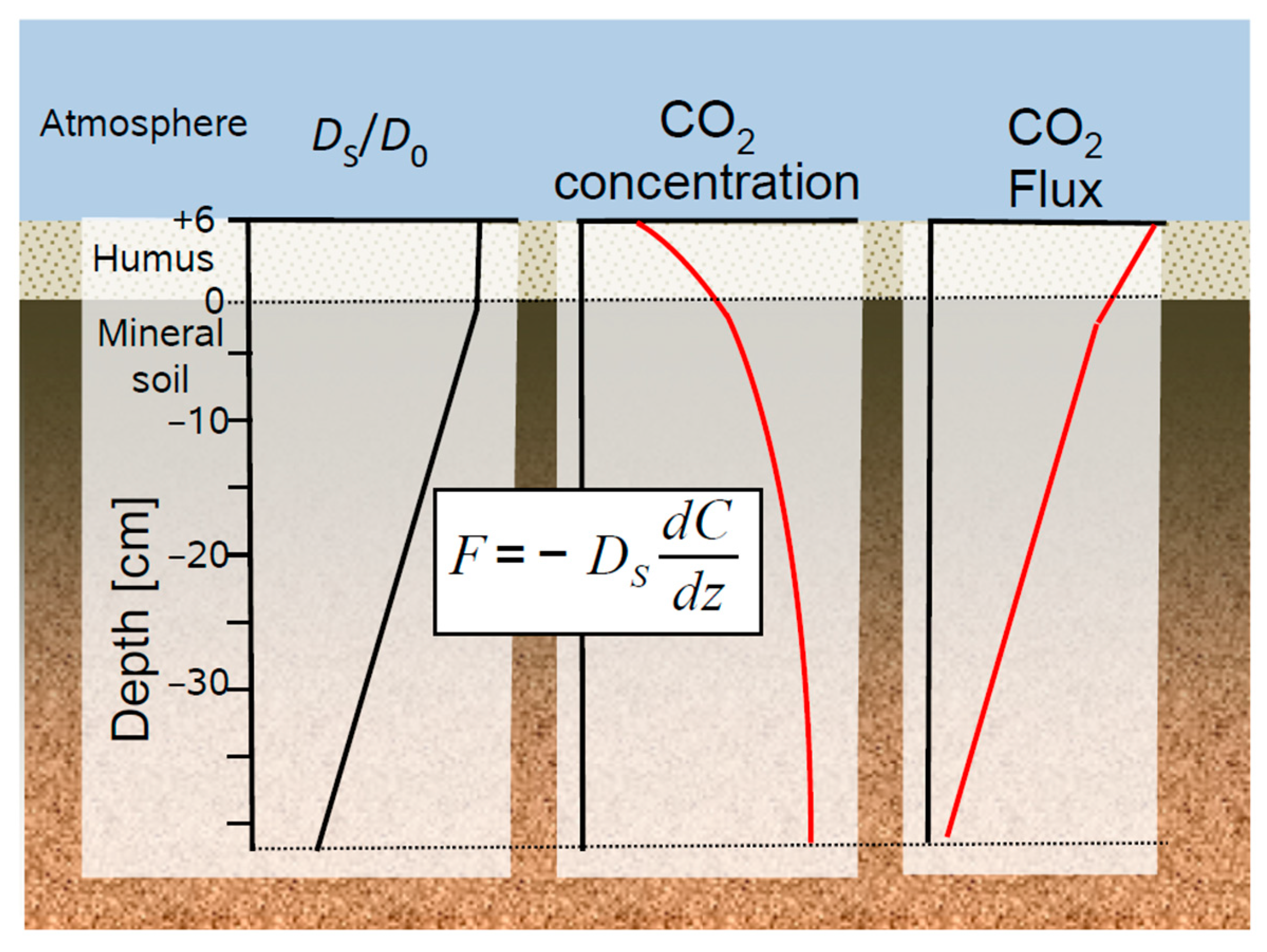
2.2.1. Theoretical Background

Soil gas monitoring provides data like soil gas concentration that can be interpreted directly, e.g., elevated concentrations of N₂O or C₂H₄ that indicate ongoing denitrification or elevated activity of certain microbes. If soil gas concentrations are linked with their exact sampling position and the transport conditions in the soil, gas flux and gas production can be calculated using the gradient method [44,50] (Figure 2). Using the gradient method implies that molecular diffusion is the dominating gas transport process in the soil. This means other gas transport processed like mass flow of air [79] and turbulence induced pressure-pumping [80,81] need to be ruled out. These processes can play temporarily a role in highly porous soils and high wind speed, yet their average contribution is probably small.

Gas diffuses in all directions, which would require a three-dimensional mathematical consideration of gas diffusion in soils [16,22]. In most cases, however, a reduction of the soil profile to a one-dimensional representative simplification is justified and common practices in soil chemistry, soil physics and hydraulic modelling. Hence, gas transport in the soil is often approximated by Fick’s first law, which is reduced to its one-dimensional formulation.

$$F=-D_{\mathrm{S}}{\rho }_{air}\frac{\partial {\chi }_C}{\partial z},$$

(1)

where F is the gas flux (mol m⁻² s⁻¹) at the depth z (m), D_S the effective gas diffusion coefficient of the gas species in the soil (m² s⁻¹), ${\rho }_{air}$ the mean air density (μmol m⁻³), ${\chi }_C$ the molar fraction (e.g., atmospheric CO₂ = ${\chi }_{C{O}_2}$ = 440 ppm or 440 µmol mol⁻¹) of the diffusing gas species at depth z. It is this gradient in molar fraction which drives molecular diffusion, and not the gradient in molar density ($C_{C{O}_2}$; µmol m⁻³) [44,82]. The net production of a gas in soil profile must suffice the conservation of matter, that means:

$$\frac{\partial C_{\mathrm{s}\mathrm{u}\mathrm{m}}}{\partial t}=-\frac{\partial F}{\partial z}+P,$$

(2)

where C_sum is the amount of gas molecules per soil volume (μmol m⁻³), t is time (s), and P the gas production (μmol m⁻³ s⁻¹) Theoretically, C_sum includes the amount of gas in air-filled pores and dissolved in the soil solution, since gas molecules exchange between these compartments. Practically, the dissolution of most trace gases is negligible, if the dissolution of CO₂ in a carbonated soil solution is excluded [65,83].

In most situations and for most gases diffusion can be assumed to be at quasi steady-state [65], so that the change in the amount of gas molecules in a soil volume can be neglected (∂C_sum/∂t = 0). Thus, we can simplify Equation (2) and combine it with Equation (1) so that

$$P=\frac{\partial }{\partial z}\left(-D_S{\rho }_{air}\frac{\partial {\chi }_C}{\partial z}\right) \approx \frac{\partial }{\partial z}\left(-D_S\frac{\partial C}{\partial z}\right),$$

(3)

${\rho }_{air}$ may result from strong temperature gradients in the soil, which can be observed as daily cycles in the top soil layer in deserts. In forest soils, however, these gradients in ${\rho }_{air}$ can be neglected, and the more common representation of the right side of Equation (3) with $\partial C/\partial z$ can be used [50,60,74,84]. The gradient method can be applied for different gases that are measured in a soil profile and which may have different order of magnitudes and even opposite directions. It is important to consider that each flux calculation requires the respective $D_S^i$ of the diffusing gas i.

2.2.2. Estimation of Soil Gas Diffusion Coefficients

Soil gas diffusion coefficients are needed to calculate soil gas fluxes from soil gas profiles. $D_S^i$ represents the exchange coefficient of a specific gas i in the soil and depends on the pore structure of the air-filled pore space ε (m³ m⁻³) and the characteristics of the diffusing gas i. The relative gas diffusion coefficient D_S/D₀ is a dimensionless measure of the quality of the structure of soil which allows the quantification of how “easily” a gas is able to diffuse through the pore structure, and which is independent of the gas species. Multiplying this dimensionless coefficient with gas specific diffusion coefficient in free air D₀ (m² s⁻¹) allows calculating the gas specific soil gas coefficient D_S (Equation (4)), which is needed to calculate fluxes.

$$D_{\mathrm{S}}=\frac{D_{\mathrm{S}}}{D_0}{D}_0,$$

(4)

D_S/D₀ depends on the air-filled pore structure, which is often addressed as a combination of the air-filled pore volume and their effectivity to allow gas exchange. Different models have been developed that can be used to calculate D_S/D₀, from simple general functions [85,86,87,88] to functions that require knowledge of many parameters or measurements of diffusivity [89,90,91]. We used site-specific models since it is impossible to predict the best diffusivity model a priori [44]. The site-specific diffusivity models were derived from laboratory measurements of soil samples from the different sites. Several soil and humus samples were taken at different depths using 100 cm³ soil cores. The porosity of the cores was measured by vacuum pycnometry. Bulk density of samples was measured gravimetrically by drying at 105 °C after all measurements. Soil gas diffusivity was measured using a one-chamber method similar to the one described by Maier et al. [65]. We used exponential functions as described by Troeh et al. [85] to parameterize our site-specific and soil-layer specific gas diffusivity functions [92]. Using these site-specific gas diffusivity functions allowed calculating the time series of D_S/D₀ from the air-filled pore-space, which in turn can be calculated as the difference between the total pore-volume and the soil water content. Using Equation (4) allows deriving D_S from D_S/D₀. Since the speed of diffusion is affected by temperature T (K) and barometric pressure p (Pa) D₀ has to be corrected for T and p.

$$D_0\left(T,p\right)=D_0^{norm} \left(\frac{p_{norm}}{p}\right){\left(\frac{T}{T_{norm}}\right)}^{\alpha },$$

(5)

where $D_0^{norm}$ is D₀ at normal barometric pressure p_norm and normal temperature T_norm, and α is a gas specific exponent between1.5 and 2 [93]. Including Equation (5) in Equation (4) allows accounting for the changing environmental conditions on molecular diffusion.

2.2.3. Measurements and Modelling of Soil Water Content

The routine program at our monitoring sites includes in situ measurements of environmental parameters at the plot and reference measurements on top of a tower or at an area nearby without forest. These continuous measurements include basic meteorological measurements such as air temperature, relative humidity, barometric pressure, wind speed, and precipitation. Soil moisture is measured as volumetric soil moisture content by ML2 and Ml3 probes (Delta-T Devices, Cambridge, UK) at 15, 30 and 60 cm depth and as soil matric potential using pF-probes (pF-Meter, EcoTech GmbH, Bonn, Germany, GeoPrecision GmbH, Ettlingen, Germany), which included soil temperature measurements.

We used the process-based, one-dimensional soil-vegetation-atmosphere-transport model LWF-Brook 90 [94] to model the water balance at our sites. LWF-Brook 90 was used to simulate daily evapotranspiration and soil water fluxes, along with soil water contents and soil water potentials within a soil profile. Evapotranspiration was calculated by a modified version of the approach by Shuttleworth and Wallace [95]. Soil-hydraulic properties were parameterized using the expressions of van Genuchten [96] and Mualem [97] The soil profile is represented by multiple layers, and the vertical water movement through these layers is described by the Richards equation [98]. The discretization of the soil profile ranged from 1 cm in the humus layer and in the upper soil to 20 cm in the subsoil. The model was parameterized using field measurements and typical parameter values [99,100,101]. The model was calibrated against time series of daily measurements of soil water content, soil matric potential and canopy throughfall. The modeled soil moisture data were used to calculate soil gas diffusivity profiles for all days including the days of the soil gas sampling.

2.2.4. Calculation Approaches for Soil Gas Fluxes

Even though the mathematical-physical description included in the gradient-flux method is valid and accurate, there are uncertainties that come with the practical implementation that need to be considered. They result from uncertainties in laboratory measurements of soil physical properties (total pore volume, diffusivity), in situ measurements and modelling (soil water content, soil gas concentration). In addition, spatial heterogeneity and discrete sampling (in time and space) allows only for grasping a snapshot of the reality.

There are different practical approaches to calculate soil gas fluxes from discrete soil gas profiles [44] that were developed to address different challenges [50,60,64,102]. The calculation approach can substantially affect the calculated efflux and the partitioning within the profile [76] and should be carefully chosen. To test and demonstrate the effect of the calculation approach on gas flux estimations we included four different approaches.

Soil gas fluxes were calculated at defined depths by multiplying the gas concentrations gradients with D_S of the respective soil layer (Equation (1)). Soil and humus were split into three layers with constant total pore volumes: humus layer, 0 to 5 cm depth, and 5 to 10 cm depth. Total pore volume and soil water content were input data to our site and depth specific diffusivity models to calculate profiles of D_S/D₀. Including D₀ allowed deriving the D_S of each gas (Equations (4) and Equation (5)). D₀ was adjusted to the current temperature and barometric pressure [93], which was derived from a weather station nearby of the German Meteorological Service (DWD) and corrected for differences in altitude when own pressure measurements were lacking. The harmonic mean of the Ds profile between the respective gas sampling depths was calculated as representative average of the respective soil layer [103].

In contrast to many other studies, we had five soil gas samplers per depth at four to five different depths in the soil to obtain a representative gas profile in the humus layer and the top 10 cm of the mineral soil. If only one concentration measurement per depth is available, as in other studies, the calculation of the concentration gradients in the soil is a simple approach of discrete differences [50,64]. With several measurements per depth different regression approaches can be used [44,76]. The same D_S/D₀ data were used for all flux calculation approaches. The first approach is based on local linear regressions (LL) that is done for all soil layers separately [76], i.e., all concentration measurements from 10 to 5 cm depth were used to calculate a representative concentration gradient for the respective layer using a simple linear regression function. The same was done for the −5 to 0 cm layer, and then the humus layer. The second approach is a linear regression (LR) across the entire soil gas profile for which all concentration measurement from the atmosphere to 10 cm depth were used to calculate one average concentration gradient for the entire profile [64]. As third approach, we used a linear spline function (LS) with a node at the soil-humus interface (0 cm depth) and at 5 cm depth in the mineral soil. The derived fluxes of the LL and LS approach were assigned to the middle of the respective layers. The fourth approach fits an exponential function (EF) for the entire concentration profile [60]. The soil–atmosphere flux of CO₂ and CH₄ was calculated using all four approaches to compare the different calculation approaches. Since the LL and LS calculation approaches are not able to estimate the concentration gradient at the soil-atmosphere interface directly, the flux estimations in the humus layer and in the 10 to 5 cm depth layer were used to extrapolate the flux to the surface [104]. The LR approach only yields one concentration gradient for the entire profile, so it could not be extrapolated. For EF the gradient at the atmosphere-humus interface was used.

For the detailed interpretation of typical patterns of soil gas fluxes we present LL derived flux estimates, unless it is stated otherwise. The LR approach was used to calculate O₂ fluxes since the lower relative measurement precision of O₂ concentrations required an approach that was less sensitive to possible outliers. It is generally assumed that the organic layer hardly contributes to CH₄ consumption [105]. Thus, negative soil CH₄ fluxes (CH₄ consumption) were not extrapolated to the soil surface but calculated directly from the observed CH₄ gradient in the humus layer. We considered the uncertainty of the estimation of the diffusivity and of the concentration gradient to quantify the uncertainty included in the soil-atmosphere fluxes. Uncertainty of the diffusivity estimation results from the uncertainty soil water content measurement which was set to +/−2 Vol.-%, and the diffusivity model, which was not considered here. Uncertainty of the gradient estimation was calculated from the regression function for CH₄ and O₂, and based on the propagation of errors of the flux estimates for the extrapolated soil-atmosphere flux for CO₂. The statistical programming language R, Version 4.0.2 (2020-06-22) [106] was used for data processing unless stated otherwise, including the packages ggplot2 [107] and dplyr [108].

2.3. Monitoring Sites

FVA-BW manages and maintains 13 monitoring plots at 6 different sites (Figure 3,

Table 2. Monitoring sites including soil gas monitoring managed by FVA-BW. Data represent annual average values.

Site	Acronym	Plot	Latitude	Longitude	Altitude (m)	Precipitation (mm)	Temperature (°C)
Rotenfels	RO	1	48.82°	8.40°	600	1258	9.0
Altensteig	AL	2	48.59°	8.63°	512	821	8.5
Conventwald	CO	2	48.02°	7.97°	810	1385	8.3
Esslingen	ES	2	48.76°	9.43°	348	781	9.6
Heidelberg	HD	3	49.45°	8.75°	510	1113	7.4
Ochsenhausen	OC	3	48.01°	9.96°	680	1111	8.6

and

Table 3. Description of the forest stands and soils at the monitoring plots. Soil types were classified using the World Reference Base for Soil resources [110].

Forest Stand			Soil				Humus
Plot	Age	Height (m)	Type	pH	Texture	Coarse Soil (%)	Type	Depth (cm)
RO spruce	128	37.2	Hyperalbic Podzol	2.94	Su3	25	Rawhumus (ROR)	15
AL spruce	110	37.1	Haplic Cambisol	3.26	Sl3	5	Mull (MUO)	8
AL beech	138	28	Stagnic Cambisol	3.77	Sl3	1	Mull (MUO)	6
CO spruce	98	34	Haplic Cambisol	3.43	Sl4	80	Moder (MOT)	10
CO beech	138	31.5	Skeletic Cambisol	3.1	Ls2	50	Moder (MOT)	3
ES spruce	110	41.9	Vertic Stagnosol	3.24	Ls2	0	Moder (MOT)	6
ES beech	138	33.2	Haplic Stagnosol	3.61	Sl4	2	Mull (MUF)	4
HD spruce	108	32.3	Haplic Cambisol	2.87	Sl3	10	Moder (MOT)	7
HD* spruce	108	32.3	Haplic Cambisol	2.87	Sl3	10	Moder (MOT)	7
HD beech	83	27.5	Haplic Stagnosol	3.52	Ls2	1	Mull (MUF)	3
OC spruce	100	33.6	Abruptic Luvisol	3.15	Lu	2	Moder (MOR)	9
OC * spruce	100	33.6	Abruptic Luvisol	4.1	Lu	8	Moder (MOR)	10
OC beech	138	36.4	Epidystric Luvisol	3.25	Ut3	2	Moder (MOR)	3

* Indicated sites received liming treatments.

) Rotenfels (RO) Altensteig (AL), Conventwald (CO), Heidelberg (HD), Ochsenhausen (OC)) in the forests of Baden-Württemberg, Germany. Of these 13 plots, ten plots at 5 sites are also listed as ICP Level 2 Monitoring plots according the ICP Forest Intensive Monitoring Program [109].

Each site has a plot of Beech forest (Fagus sylvatica. L.) and a plot of Spruce forest (Picea abies. (L) H. Karst.). The sites Heidelberg and Ochsenhausen include an additional treatment plot where the soil has been limed with CaMg(CO₃)₂ in 1984 and 1994, respectively. An additional Spruce plot was installed in Rotenfels, which is not part of the regular ICP Level 2 monitoring program. The sites and plots were selected to represent the typical forest regions of Baden-Württemberg and the most frequent local broadleaved tree (beech) and conifer species (spruce). All plots have been established before 1995 and are managed according to the guidelines for the ICP Level 2 monitoring program Soil gas monitoring started in 1998 on 8 plots and 2010 on 5 plots.

The plots are covered by homogenous forests stand of approximately 0.25 ha (Table 3). The spruce plot and the beech plot are located next to each other. The management routine includes a combination of in situ measurements by permanently installed sensors and data loggers and repeated sampling (automatic and manual) on a regular scheme and subsequent analysis in the laboratory. Infrastructure and routines for soil gas monitoring have been established in addition to the internationally harmonized monitoring routine of the ICP Forest monitoring network. For the presentation of exemplary results we used data of the spruce plot of the ES site from the years 2005–2020.

3. Results and Discussion

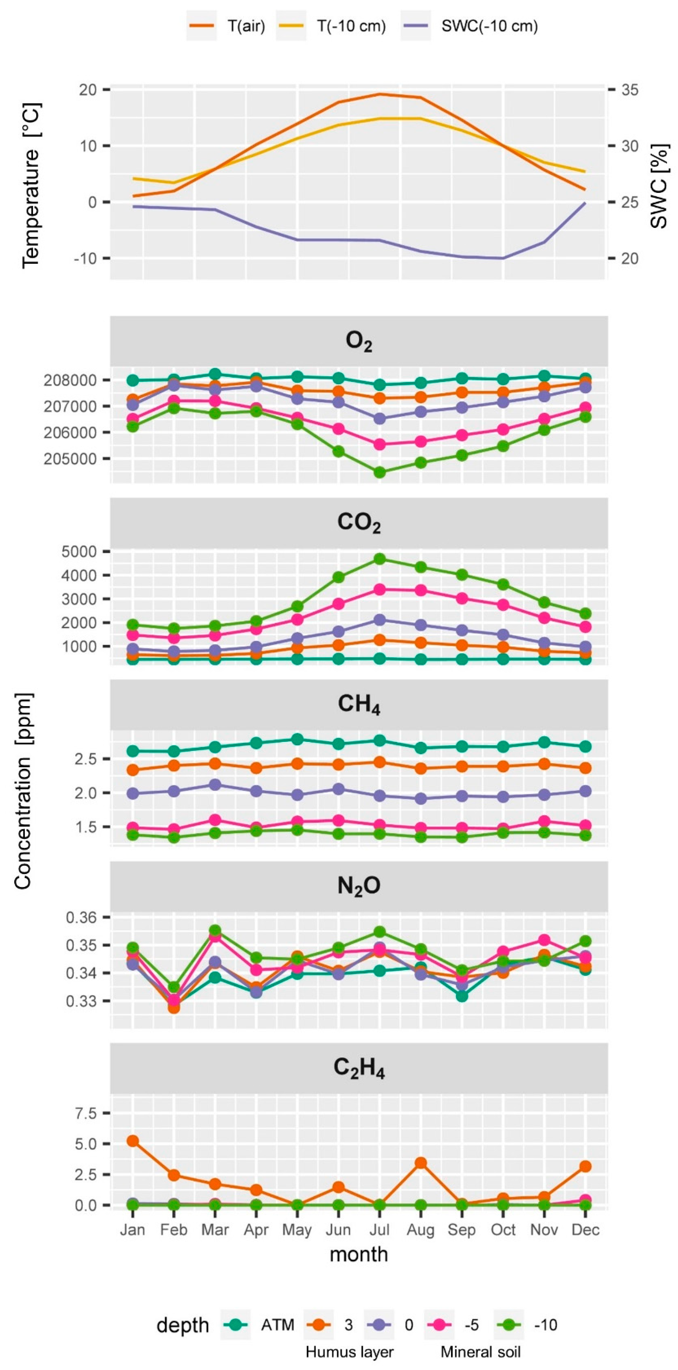
3.1. Time Series of O₂, CO₂, CH₄, N₂O and C₂H₄ and Typical Soil Gas Profiles

3.1.1. Time Series and Seasons

We present typical examples and interpretations of selected data from the Spruce monitoring plot at the ES site (Figure 4). All data were quality checked and filtered so that the different gases presented in this example cover different time slots. N₂ and Ar are not shown since they were only used for quality assurance purposes.

O₂ concentrations always decreased with depth indicating consumption of O₂ by the soil (Figure 4). A clear seasonality in O₂ concentrations was registered (Figure 5) with O₂ concentrations reaching down to 200,000 ppm (20%), which is approx. 8000 ppm below the atmospheric concentration of O₂ (Figure 4). This means, this soil was always well-aerated. Soil CO₂ showed an opposite course and clearly increased in concentration with depth throughout the entire time series (Figure 5). CO₂ concentrations ranged from 400 ppm near the soil surface to 10,000 ppm in 10 cm depth. Soil CO₂ also shows a typical seasonality with much higher concentrations in the summer when temperatures and soil respiration is highest (Figure 5).

Atmospheric CH₄ concentrations at the ES spruce plot were higher on average (2.6 pmm) than expected and seemed to fluctuate slightly over time. Soil CH₄ concentrations always showed a strong decrease with depth indicating CH₄ consumption by methanotrophic bacteria within the soil profile.

Soil CH₄ reached concentrations as low as 1 ppm at 10 cm depth (Figure 4). CH₄ concentrations did not show a clear seasonality unlike CO₂ and O₂ (Figure 5). The relatively high atmospheric CH₄ concentrations could be due to a strong local CH₄ source e.g., an industrial area, a biogas plant or peatland. It could also partly result from the relative uncertainty of the calibration gas and other artefacts. The apparently elevated atmospheric CH₄ concentration had only an indirect effect since our monitoring and flux calculation approach rather relies on detecting vertical gradients than measuring the absolute concentration. To find out about or source of CH₄ or possible artefact we are currently planning CH₄ measurements with an independent gas analysis system. The time series of N₂O neither showed a clear seasonality nor clear depth gradients. They often showed a very weak increase in concentration with depth, yet the variability at a given depth was often in a similar range (Figure 4). Calculating a seasonal average course from the entire time series (Figure 5) showed that this weak increase with depth was persistent during most of the seasons, which is an indication of an ongoing weak mean denitrification and production of N₂O.

Reliable measurement of soil C₂H₄ concentrations (above the detection limit) could be collected only after 2017 at this site (Figure 4). Most values of C₂H₄ measurements were below the detection limit which is normal for a well aerated soil. Despite the good supply of O₂ we detected concentrations of up to 6 ppm of C₂H₄. C₂H₄ concentrations seemed to have higher values in winter (Figure 5) when soil water content was higher and soil gas diffusivity lower. In summer, when soil temperature peaked and soil microbial activity was highest, C₂H₄ concentrations also seemed to become temporarily higher. The detected C₂H₄ concentrations of up to 6 ppm in the humus layer can be considered as a high value [27].

We think that the production of C₂H₄ occurs at hot spots similar to the production of N₂O. This is in contrast to the more or less evenly distributed production CO₂ or consumption of O₂ which results in more homogenous soil gas profiles. Calculating C₂H₄ fluxes or production rates was not feasible due to the limited data and its small-scale processes. Nevertheless, studying the dynamics and spatiotemporal patterns of the C₂H₄ data at all 13 monitoring plots promises new insights in intensity and frequency of situations during which C₂H₄ is produced in forest soils. The analysis of long term C₂H₄ data will allow the identification of drivers and effects, such as drought, liming, enhanced mineralization, waterlogged soils and biotic stressors.

3.1.2. Typical Soil Gas Profiles

Soil water content, soil temperature and soil gas diffusivity are important drivers and underlay seasonal cycles (Figure 5 and Figure 6). D_S/D₀ is highest in the humus layer and lower in the deeper mineral soil layers (Figure 6 top). This is an effect of the decrease in total pore space with depth which results from the load of the soil above [45,65]. D_S/D₀ is decreasing with depth within each layer because soil water content is usually increasing with depth. The typical D_S/D₀ profile changes through the seasons. The wet seasons of spring and winter have higher soil water contents and thus lower D_S/D₀ values than the warmer and drier seasons of summer and fall (Figure 5 and Figure 6).

Soil gas profiles data (O₂, CO₂, CH₄ and N₂O) were grouped according to their season (Figure 6). Seasonal average values per sampler were calculated instead of monthly averages of all five samplers per depth (as shown in Figure 5) to represent the variability covered by the replications. That means variability of the green dots at a given depth shown in Figure 6 represents the average spring concentration of one specific sampler at a given depth. This allows assessing the homogeneity of the soil gas profiles and gives some information on possibly simultaneously occurring processes

O₂ decreased with depth in all seasons, similar to the increase in CO₂ with depth. The CO₂ and O₂ gradients are much stronger in summer than in winter and spring. Average summer concentrations of CO₂ and O₂ of all samplers are clearly different from winter concentrations (blue and yellow dots do not mix), because the strong seasonal cycle dominates the variability of each sampler at all depths. The O₂ gradient is strongest during summer and lowest O₂ values were registered in 10 cm depth in the summer seasons, as observed in the seasonal time course of soil gas concentrations (Figure 4). Seasonal soil CO₂ concentrations were very similar to the O₂ profiles but had slightly bigger differences between the winter and spring profiles than the O₂ data (Figure 6). The CO₂ concentrations of all samplers showed a persistent ranking over time according to their depth, but also at each depth (data not shown). The lower absolute precision of the concentration measurement of O₂ compared to CO₂ resulted in a slightly larger scattering of daily profiles, which was smoothed out by averaging seasonal O₂ profiles in Figure 5 and Figure 6. Yet, daily O₂ profiles included a higher uncertainty in the concentration measurement than CO₂ profiles.

The seasonal soil CH₄ concentrations showed an almost constant profile all year round with a linear decrease in CH₄ concentration from the soil surface to 5 cm depth (Figure 5 and Figure 6) which means that the gradients did not vary too much over time and within the top soil. One of the five samplers at 10 cm depth had average CH₄ concentrations from 1.7 to 1.8 ppm throughout the seasons while all other samplers always had CH₄ concentrations below 1.5 ppm. This indicates either (a) a weak local net production of CH₄ near this sampler while net consumption of CH₄ dominated the rest of the soil gas profile, (b) less CH₄ consumption above this sampler, or (c) a locally higher soil gas diffusivity above the sampler. Since also CO₂ and O₂ concentrations of this gas sampler were closer to atmospheric concentrations, (c) is most probable. CH₄ concentrations of all samplers showed a persistent ranking over time as observed for CO_2. This persistence of the ranking over time is a clear hint that our sampling and measurements are highly reproducible and that our set-up allows detecting even small changes in the dynamics of soil gases.

Time series of the seasonal N₂O concentrations at a depth (Figure 4 and Figure 5) and seasonal profiles (Figure 6) showed a high variability in the N₂O profile and a large overlap of concentrations between the seasons. Averaged monthly atmospheric N₂O concentrations ranged from 324 to 340 ppb (Figure 5 and Figure 6) which is half the variability as observed within the soil profile (324 to 361 ppb). Even if an increase of N₂O concentrations with depth might be apparent from Figure 5 and Figure 6, we have to consider that the variability of N₂O concentrations at each depth is larger than the profile gradient (Figure 6). The weak increase in N₂O concentrations in the mineral soil indicates a weak ongoing production of N₂O. Yet, the N₂O gradient in the humus layer was sometimes negative and sometimes positive, and often weak and not significant. This can result from (a) insufficient precision of the measurement, (b) intrinsic variability of the soil gas profile resulting from small scale processes, or (c) absence of N₂O production or consumption. Regarding (a) we conclude that the observed average N₂O profiles of approx. 10 ppb can be reliably detected considering the measurement precision of N₂O of approximately. 3.6 ppb (Table 1). The even larger variability of 10–20 ppb between the replication samplers at each depth indicates that the lack of statistical significance in of the overall soil N₂O gradient results from (b) simultaneously occurring small scale production and consumption of N₂O. Forest soils can take up atmospheric N₂O [19]. This would be in agreement with the sub ambient concentrations [16,42] which were observed in the humus layer from time to time. Measurement of N₂O uptake is generally very difficult since N₂O uptake rates are usually very low and often below the detection limit of regular chamber measurements [42,111]. We also observed N₂O concentrations in the humus layer above atmospheric concentrations from time to time which would indicate a net production of N₂O. N₂O concentrations in forest soils can reach up to several ppm [76,112]. Especially in agricultural soils, N₂O fluxes can be very high after flooding or fertilization [113]. High N₂O concentrations were also observed from time to time at our other soil gas monitoring plots, especially during periods of enhanced mineralization of the humus layer (data not shown). The observed N₂O concentration profiles at this plot, however, did not show strong gradients and possible emissions or consumption could not be calculated. The N₂O balance of a forest or agricultural site rather depends on catching the peak events [113,114], than spanning the potentially long time between the peak events when fluxes might be negligible. A regular schedule might thus be a drawback. Covering long time series which combine discrete measurements (soil gas) and continuous measurement (temperature, soil moisture), on the other hand, allows to stochastically estimate the probability of N₂O peak emissions events and to identify the drivers. This would allow then modelling the undetected peaks using the continuous proxies.

3.2. Effect of Different Calculation Approaches for Gas Flux Estimation

3.2.1. Comparison of Calculation Approaches

Four different calculation approaches for the estimation of the soil-atmosphere gas flux were compared. For the comparison CH₄ and CO₂ concentration data were used. Soil respiration estimates of all four approaches yielded similar values, while the effect of the calculation approach was more pronounced for the CH₄ consumption estimation (Figure 6, middle, right). The ranking between the different approaches was the same for soil respiration and CH₄ consumption: the LR approach yielded the lowest soil respiration and CH₄ consumption estimates followed by EF approach. Estimates of the LL and LS approach were very similar. While other comparisons [76] found large overestimation by the EF approach, we observed substantially lower flux estimates for the EF, but only for CH₄ and not CO₂.

We explain the consistency of the different approaches by the linear shape of the CO₂ profile in the top soil (Figure 5) that can be appropriately fit and reflected by all four approaches. Other studies have also taken into account the concentrations at deeper depths [60,76,84]. These concentration measurements at greater depth have a mathematical effect on the calculation of the concentration gradient at the soil-atmosphere interface although they have practically no influence at all on the actual concentration gradient at the soil-atmosphere interface. It could be shown that the inappropriate use of the EF approach can lead to substantial overestimation of the efflux estimates [76]. Thus, the consistency of the different calculation approaches in our case can be interpreted as a robustness or independence of the CO₂ concentration gradient from the calculation approach, which is due to the shallow soil gas profile that focuses on the top 10 cm of the mineral soil and humus layer.

However, the four different approaches had a substantial effect on the estimation of the CH₄ consumption (Figure 7, middle). Visual inspection of (Figure 7 left) shows that the more flexible LL and LS approaches can better fit the concentration data in the humus and yield a stronger CH₄ gradient, and thus higher CH₄ flux rates. The fits of EF and LR include all data that means also concentrations between 10 and 0 cm depths where obviously another CH₄ gradient can be observed. The LL and LS approach yielded similar results (Figure 7, middle) and both approaches allow calculating soil gas fluxes at different depths. The LL approach however can be challenged more easily by soil gas profiles with weak gradients and outliers. We observed that under certain circumstances the LL approach yielded the same gradient in the humus layer as in the mineral soil with the regression functions shifted in parallel although a curvature was obvious in the entire soil gas profile. In such situations, the LS represented the overall curvature in a more realistic way, since it guarantees a continuous function.

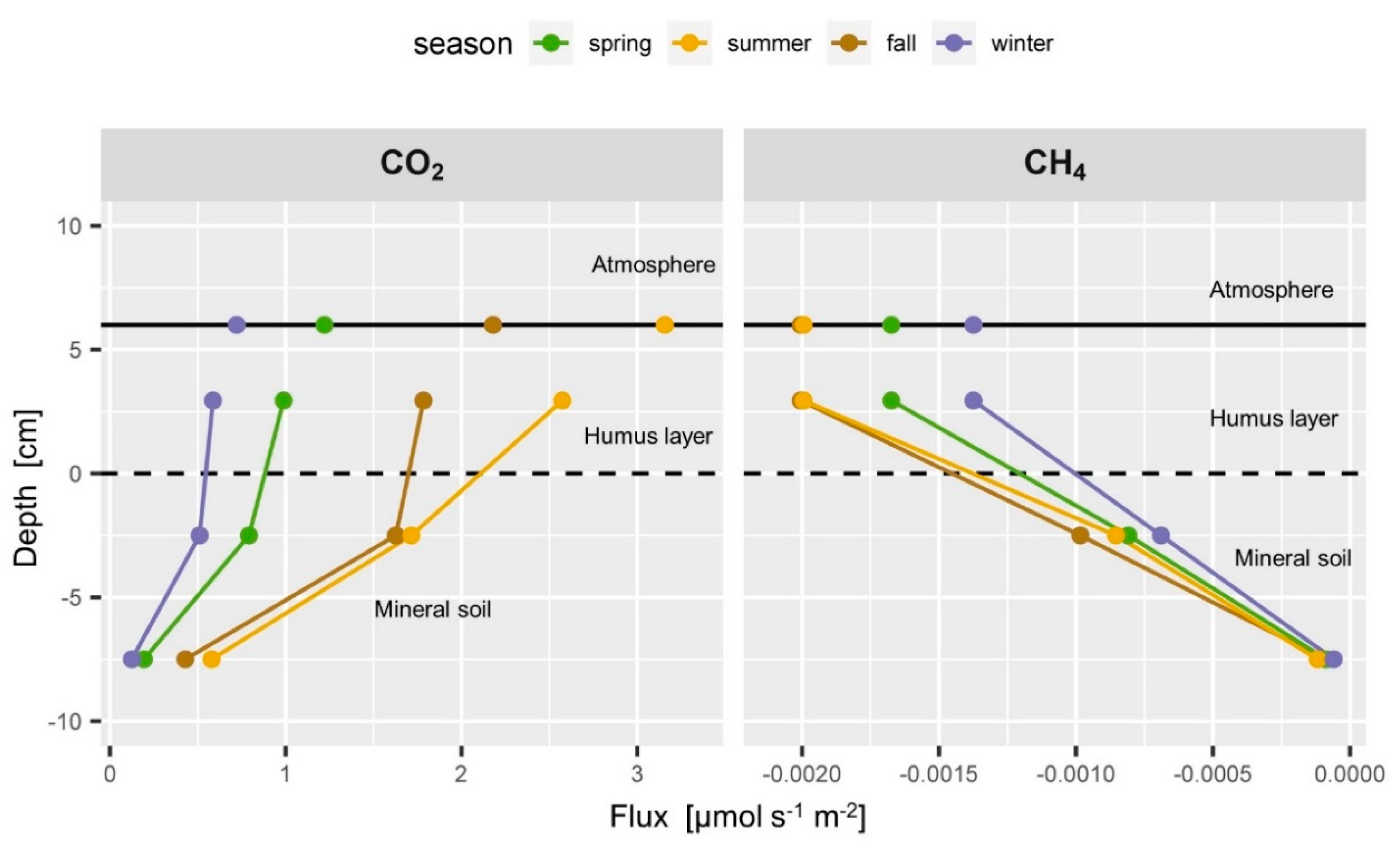
3.2.2. Vertical Partitioning of Soil Gas Fluxes

We used the LL method to derive concentration gradients at different depth for CO₂ and CH₄ (Figure 6), which allows calculating vertical profiles of soil gas fluxes (Figure 8) and allocating the production and consumption of gases to a certain depth [44,60]. The increase in the CO₂ flux between the 10 to 5 cm depth layer and the humus layer was extrapolated to the soil-atmosphere interface (Figure 8 left) as proposed by Hirano et al. [104]. CO₂ flux between 10 to 5 cm depth was usually <20% of the estimated efflux. Soil CO₂ fluxes always increased towards the soil surface. The increase in the CO₂ flux between the 5 to 0 cm depth layer and the humus layer was lower during the colder seasons (fall to spring) than in summer when the topsoil was warm. This higher soil respiration rate can be explained at least partly by the enhanced decomposition of organic material in the humus layer during summer. The top mineral soil and humus layer contributed the largest fraction of the total soil respiration as observed by others [11,16,60,84]. Future detailed analysis of the soil gas monitoring data will allow studying the temporal evolution of soil respiration in the mineral soil and the humus layer and their contribution to the total respiration. Such analysis holds the potential to better quantify the dynamics of the mineralization of the humus layer and better understand the C cycle in the soil.

The soil-atmosphere flux of CH₄ was set to the estimated CH₄ flux in the humus layer (Figure 8, right) since it can be expected that CH₄ consumption in the top cm of the spruce litter does not contribute substantially to CH₄ consumption [16,105]. The CH₄ flux between 5 and 10 cm depth was very low, which corresponds to the very weak gradient compared to the gradient observed above (Figure 6 and Figure 7 left). The negative soil CH₄ fluxes increased almost linearly from the 10 to 5 cm depth to the humus layer during all seasons (Figure 8 right). More than 90% of the CH₄ was consumed in the top 10 cm of the mineral soil. This corresponds to the observation that the topsoil is the most active CH₄ consumer [16,105]. The CH₄ flux profile showed an apparent seasonality with higher consumption rates in summer and fall than in winter, which resulted from the seasonal changes in soil moisture and soil gas diffusivity (Figure 6 and Figure 7).

The soil O₂ profiles did not allow using the LL or LS approach since they randomly yielded unrealistic flux estimates from time to time where O₂ fluxes in the mineral horizon seemed to be higher than in the humus layer above. Reducing the degree of freedom by using the LR approach instead allowed stabilizing the estimation of the O₂ gradient. This approach is suitable if the observed concentrations gradients are weak due to limited precision of the O₂ measurements, and if the assumption of more or less linear gradients is justified based on prior knowledge. The comparison of the calculation approaches could show that the LR and LS approach yield very similar results for the estimation of the soil-atmosphere flux of CO₂. Since O₂ fluxes mainly counterbalance CO₂ fluxes [115], it would be reasonable to assume that the LR approach is suitable for calculating the O₂ gradient.

N₂O data can also be characterized by problematic soil gas profiles that hardly exhibit significant concentration gradients, or profiles with very weak gradients (Figure 6, bottom) [16,76]. Even though O₂ profiles and N₂O profiles might yield a similar statistical result in terms of the quality of the regression (e.g., R²), they have to be interpreted differently. Production and consumption of N₂O can occur on very small spatial scales [16], and even within aggregates and other hot spots [15], so that “noisy” N₂O profiles are a result of really ongoing processes. O₂ is primarily consumed by microbes and counterbalances soil respiration which originates more or less evenly distributed from the entire topsoil. We think that the scattering in the O₂ profiles results to a larger extent from the lower precision of the measurement, which can be improved by repeated measurements (LR approach). Estimating surface fluxes of N₂O includes thus a higher uncertainty than O₂ fluxes although the estimation of their concentration gradients might yield a similar R². As a consequence, we used the LS and LL approach for soil gas profiles that allowed calculating flux rates at different depths (CO₂ and CH₄) and LR for the estimation of O₂ fluxes which require a more robust approach. N₂O fluxes were not calculated since the uncertainty requires additional quality assurance like comparative chamber measurements, which is currently planned.

3.3. Time Series and Interaction of Soil-Atmosphere Fluxes of O₂, CO₂ and CH₄

3.3.1. Time Series Soil-Atmosphere Fluxes

Soil-atmosphere fluxes of O₂ and CO₂ showed a strong seasonal behaviour (Figure 9) as observed from the soil gas profiles (Figure 5), with high flux rates during summer where temperatures were highest and soil moisture usually lowest (Figure 9). The time course of O₂ seemed to reflect inversely the time course of CO₂. CO₂ emissions and O₂ consumption reached from values close to zero up to approximately 6 µmol m⁻² s⁻¹, and had an average flux of 1.97 µmol CO₂ m⁻² s⁻¹ and of 1.95 µmol O₂ m⁻² s⁻¹. This flux corresponds to 746 g C m⁻² yr⁻¹ which is an average value for temperate forests [116,117].

Our soil respiration data represent an ideal base for further investigation e.g., the quantification of the effect of the environmental drivers such as soil temperature and soil moisture (Figure 9) [12,28] or the relationship between soil respiration and tree growth [37]. Working with the time series of all 13 soil gas monitoring plots will also allow comparing the effect of different trees, e.g., beech vs. spruce [117], and forest dynamics like thinning or drought effects.

Soil-atmosphere fluxes of CH₄ showed more variability than soil CH₄ concentrations, yet obvious seasonal cycles as observed with CO₂ and O₂ fluxes were not observed. Soil CH₄ consumption ranged between 0.001 and 0.003 µmol m⁻² s⁻¹, which is in the range of CH₄ consumption rates observed in the region [41,72]. The average yearly consumption of 8.08 kg CH₄ ha_-1 yr⁻¹ corresponds to a high value (top 25%) compared to temperate forest soils worldwide [18]. Future detailed analysis of the CH₄ profiles and fluxes of all sites will allow studying the temporal evolution and long-term changes of CH₄ consumption. This is of special interest since it is currently under debate that soils might be losing their capacity to consume atmospheric CH₄ as recently observed by Ni and Groffman [118].

The uncertainty in the CO₂, O₂ and CH₄ fluxes estimation changed over time (Figure 9) and resulted from the uncertainty in the gradient estimation and measurement of the soil water content. The uncertainty in CO₂ and O₂ fluxes seemed to be much smaller than in the CH₄ fluxes which is due to the stronger gradients and less scattering in the data (Figure 6 and Figure 7). The estimation of the uncertainty is not fully comparable between the CO₂ and O₂ fluxes since their calculation approach (LR vs. LL) was different and a different number of data points were used for the calculation of the gradient.

The relative contribution of the measurement uncertainty of the soil water content was constant over time, so that changes in the total uncertainty of flux estimates originate directly from the estimation of gradients in the gas concentration profiles. If the gradients in the respective soil gas profile become less distinct due to more scattering of the concentrations, the uncertainty in the flux estimation increases, e.g., the summer peak in soil CO₂ efflux in 2013 (Figure 9). The uncertainty in the parameter estimates of the diffusivity model would be an additional source of uncertainty which was not included so far. In situ measurements of soil gas diffusivity would allow to assess the quality of the diffusivity models [69,81] and improve the gradient based flux estimates. Additionally, chamber measurements next to the soil gas profiles would allow comparing and evaluating the gradient based flux estimates and also the diffusivity model [77].

3.3.2. Relationship of O₂ and CO₂ Fluxes

O₂ and CO₂ fluxes fell close to the diagonal −1:1 line (Figure 10), which means O₂ fluxes and CO₂ fluxes were well counterbalanced. Individual data points from winter and spring deviate substantially from the 1:1 line. This can be a result of a failure in the estimation of the O₂ gradients, or can be an actual ongoing process [115]. The ratio of the soil CO₂ efflux to the soil O₂ flux can be addressed as apparent respiratory quotient (ARQ) [119]. ARQ is often close to 1 [115,120] if transport mechanisms like the export of dissolved CO₂ or other relevant processes such as intensive weathering of minerals in the soil can be ruled out. Studies found ARQ values < 0.7 in Mediterranean ecosystems [119] and that even up to 2/3 of the soil respiration can be lost via subsurface processes [121]. At the ES site soil respiration seemed to be well counterbalanced by an equimolar O₂ flux so that CO₂ losses due to subsurface processes can be ruled out. Dissolution of soil CO₂ in soils with pH > 7 can play an important role [9,83,119]. Yet, the soil at the ES site is acidic and dissolution and export of soil CO₂ via percolating water plays only a negligible role.

Future detailed analysis of soil gas monitoring data will allow studying ARQ to evaluate the relevance of subsurface processes at the different sites. Studying the temporal evolution of ARQ and O₂ concentrations might give new insights into processes at temporarily waterlogged soils which may become anoxic for a certain time [120].

4. Conclusions

We introduced an experimental set-up and design for long term soil gas monitoring. Typical soil gas profiles and fluxes of one of 13 monitoring plots were presented to discuss the specifications, advantages, and drawbacks of the system. Several passive gas samplers per depth were used which allows a precise assignment of the sampling locations. This is a prerequisite for the assessment of the homogeneity of the soil gas profile and the quantification and qualification of the estimates of the soil gas fluxes. The samplers do not require electrical power or intensive maintenance and affect the soil surface only minimally which makes them ideal for long term monitoring. The soil gas samplers allow efficient and highly reproducible handling of the gas samples which is essential for a good quality assurance. The subsequent GC analysis was optimized for the purpose and additional gas analysis can be included. These features make the set-up an efficient, versatile, flexible, and reliable tool which is suitable for long-term monitoring of soil gas profiles.

The monitoring routine is scheduled from biweekly to monthly measurements for practical reasons. Such a schedule is suitable to cover seasonal cycles which are known for soil CO₂, O₂ and CH₄. The routine schedule is a drawback for occasional event-based soil gas dynamics such as N₂O fluxes that are dominated by peak events. While CO₂, O₂, and CH₄ fluxes can be reliably estimated based on their concentration profile, N₂O fluxes are more difficult to estimate especially when N₂O soil concentration gradients are weak and indicating concurrent production and consumption of N₂O at the same time within the profile. Future campaigns with chamber measurements could provide reference values of gas fluxes that can help to eliminate or minimize sources of uncertainty and add additional value to our data.

The long-term soil gas profile data of 13 forest plots and the ongoing monitoring and evaluation holds the potential to answer various research questions. It is the ideal data basis to study (a) the linkage between soil respiration, tree growth and forest productivity, (b) the interaction and drivers of soil gas fluxes of CO₂, CH₄ and N₂O, (c) the relationship of CO₂ and O₂ fluxes and potential interfering processes such as anoxic conditions, (d) the interaction between concurrent production and consumption of N₂O, and (e) appearance and drivers of C₂H₄ in forest soils. The continuity of the existing long term records soil gas data in combination with the ICP Forest Level 2 monitoring program are the ideal basis for further ecophysiological studies related to soil processes in which soil gases are produced or consumed.

References

1. Wang, B.; Brewer, P.E.; Shugart, H.H.; Lerdau, M.T.; Allison, S.D. Soil aggregates as biogeochemical reactors and implications for soil-atmosphere exchange of greenhouse gases—A concept. Glob. Chang. Biol. 2019, 25, 373–385. [Google Scholar] [CrossRef] [PubMed]
2. Chesworth, W. Encyclopedia of Soil Science; Springer: Dorderecht, The Netherlands, 2009; p. 902. [Google Scholar]
3. Smith, K.A.; Ball, T.; Conen, F.; Dobbie, K.E.; Rey, A. Exchange of greenhouse gases between soil and atmosphere: Interactions of soil physical factors and biological processes. Eur. J. Soil Sci. 2018, 69, 2–4. [Google Scholar] [CrossRef]
4. IPCC. Climate Change 2013: The Physical Science Basis. Contribution of Working Group I to the Fifth Assessment Report of the Intergovernmental Panel on Climate Change; IPCC: Cambridge, UK; New York, NY, USA, 2013.
5. Conrad, R. Soil microorganisms as controllers of atmospheric trace gases (H2, CO, CH4, OCS, N2O, and NO). Microbiol. Rev. 1996, 60, 609–640. [Google Scholar] [CrossRef] [PubMed]
6. Sánchez-Cañete, E.P.; Kowalski, A.S.; Serrano-Ortiz, P.; Pérez-Priego, O.; Domingo, F. Deep CO2 soil inhalation/exhalation induced by synoptic pressure changes and atmospheric tides in a carbonated semiarid steppe. Biogeosciences 2013, 10, 6591–6600. [Google Scholar] [CrossRef] [Green Version]
7. NOAA. Global Monitoring Laboratory Earth System Research Laboratories. Available online: https://www.esrl.noaa.gov/gmd/ccgg/trends/ (accessed on 22 November 2020).
8. Ryan, M.G.; Law, B.E. Interpreting, measuring, and modeling soil respiration. Biogeochemistry 2005, 73, 3–27. [Google Scholar] [CrossRef]
9. Maier, M.; Schack-Kirchner, H.; Hildebrand, E.E.; Schindler, D. Soil CO2 efflux vs. soil respiration: Implications for flux models. Agric. Meteorol. 2011, 151, 1723–1730. [Google Scholar] [CrossRef]
10. Chen, L.; Liu, L.; Qin, S.; Yang, G.; Fang, K.; Zhu, B.; Kuzyakov, Y.; Chen, P.; Xu, Y.; Yang, Y. Regulation of priming effect by soil organic matter stability over a broad geographic scale. Nat. Commun. 2019, 10, 5112. [Google Scholar] [CrossRef] [Green Version]
11. Goffin, S.; Aubinet, M.; Maier, M.; Plain, C.; Schack-Kirchner, H.; Longdoz, B. Characterization of the soil CO2 production and its carbon isotope composition in forest soil layers using the flux-gradient approach. Agr. Met. 2014, 188, 45–57. [Google Scholar] [CrossRef]
12. Davidson, E.A.; Janssens, I.A. Temperature sensitivity of soil carbon decomposition and feedbacks to climate change. Nature 2006, 440, 165–173. [Google Scholar] [CrossRef]
13. Conrad, R. Soil microbial processes involved in production and consumption of atmospheric trace gases. Adv. Microb. Ecol. 1995, 14, 207–250. [Google Scholar]
14. Smith, K.A.; Ball, T.; Conen, F.; Dobbie, K.E.; Massheder, J.; Rey, A. Exchange of greenhouse gases between soil and atmosphere: Interactions of soil physical factors and biological processes. Eur. J. Soil Sci. 2003, 54, 779–791. [Google Scholar] [CrossRef] [Green Version]
15. Kuzyakov, Y.; Blagodatskaya, E. Microbial hotspots and hot moments in soil: Concept & review. Soil Biol. Biochem. 2015, 83, 184–199. [Google Scholar] [CrossRef]
16. Maier, M.; Longdoz, B.; Laemmel, T.; Schack-Kirchner, H.; Lang, F. 2D profiles of CO2, CH4, N2O and gas diffusivity in a well aerated soil: Measurement and Finite Element Modeling. Agr. Met. 2017, 247, 21–33. [Google Scholar] [CrossRef]
17. Von Fischer, J.C.; Hedin, L.O. Separating methane production and consumption with a field-based isotope pool dilution technique. Glob. Biogeochem. Cycles 2002, 16, 8-1–8-13. [Google Scholar] [CrossRef]
18. Dutaur, L.; Verchot, L.V. A global inventory of the soil CH4 sink. Glob. Biogeochem. Cycles 2007, 21. [Google Scholar] [CrossRef]
19. Chapuis-Lardy, L.; Wrage, N.; Metay, A.; Chotte, J.-L.; Bernoux, M. Soils, a sink for N2O? A review. Glob. Chang. Biol. 2007, 13, 1–17. [Google Scholar] [CrossRef]
20. Davidson, E.A.; Verchot, L.V. Testing the Hole-in-the-Pipe Model of nitric and nitrous oxide emissions from soils using the TRAGNET Database. Glob. Biogeochem. Cycles 2000, 14, 1035–1043. [Google Scholar] [CrossRef]
21. Ingwersen, J.; Butterbach-Bahl, K.; Gasche, R.; Richter, O.; Papen, H. Barometric Process Separation: New Method for Quantifying Nitrification, Denitrification, and Nitrous Oxide Sources in Soils. Soil Sci. Soc. Am. J. 1999, 63, 117–128. [Google Scholar] [CrossRef]
22. Well, R.; Maier, M.; Lewicka-Szczebak, D.; Köster, J.-R.; Ruoss, N. Underestimation of denitrification rates from field application of the 15N gas flux method and its correction by gas diffusion modelling. Biogeosciences 2019, 16, 2233–2246. [Google Scholar] [CrossRef] [Green Version]
23. Smith, A.M. Ethylene in Soil Biology. Annu. Rev. Phytopathol. 1976, 14, 53–73. [Google Scholar] [CrossRef]
24. Neljubow, D. Über die horizontale Nutation der Stengel von Pisum sativa und einiger Anderer Pflanzen. Beih. Bot. Cent. 1901, 10, 128–139. [Google Scholar]
25. Arshad, M.; Frankenberger, W.T. Ethylene in Soil; Springer: Boston, MA, USA, 2002; pp. 139–193. [Google Scholar] [CrossRef]
26. Jackson, M.B. Ethylene and Responses of Plants to Soil Waterlogging and Submergence. Annu. Rev. Plant Physiol. 1985, 36, 145–174. [Google Scholar] [CrossRef]
27. Zechmeister-Boltenstern, S.; Smith, K.A. Ethylene production and decomposition in soils. Biol. Fertil. Soils 1998, 26, 354–361. [Google Scholar] [CrossRef]
28. Davidson, E.A.; Belk, E.; Boone, R.D. Soil water content and temperature as independent or confounded factors controlling soil respiration in a temperate mixed hardwood forest. Glob. Chang. Biol. 1998, 4, 217–227. [Google Scholar] [CrossRef] [Green Version]
29. Goffin, S.; Wylock, C.; Haut, B.; Maier, M.; Longdoz, B.; Aubinet, M. Modeling soil CO2 production and transport to investigate the intra-day variability of surface efflux and soil CO2 concentration measurements in a Scots Pine Forest (Pinus Sylvestris, L.). Plant Soil 2015, 390, 195–211. [Google Scholar] [CrossRef] [Green Version]
30. Conant, R.T.; Dalla-Betta, P.; Klopatek, C.C.; Klopatek, J.M. Controls on soil respiration in semiarid soils. Soil Biol. Biochem. 2004, 36, 945–951. [Google Scholar] [CrossRef]
31. Luo, G.J.; Kiese, R.; Wolf, B.; Butterbach-Bahl, K. Effects of soil temperature and moisture on methane uptake and nitrous oxide emissions across three different ecosystem types. Biogeosciences 2013, 10, 3205–3219. [Google Scholar] [CrossRef] [Green Version]
32. Luo, G.; Brüggemann, N.; Wolf, B.; Gasche, R.; Grote, R.; Butterbach-Bahl, K. Decadal variability of soil CO2, NO, N2O, and CH4 fluxes at the Höglwald Forest, Germany. Biogeosciences 2012, 9, 1741–1763. [Google Scholar] [CrossRef] [Green Version]
33. Subke, J.-A.; Moody, C.S.; Hill, T.C.; Voke, N.; Toet, S.; Ineson, P.; Teh, Y.A. Rhizosphere activity and atmospheric methane concentrations drive variations of methane fluxes in a temperate forest soil. Soil Biol. Biochem. 2018, 116, 323–332. [Google Scholar] [CrossRef]
34. Keller, M.; Varner, R.; Dias, J.D.; Silva, H.; Crill, P.; de Oliveira, R.C.; Asner, G.P. Soil–Atmosphere Exchange of Nitrous Oxide, Nitric Oxide, Methane, and Carbon Dioxide in Logged and Undisturbed Forest in the Tapajos National Forest, Brazil. Earth Interact. 2005, 9, 1–28. [Google Scholar] [CrossRef] [Green Version]
35. Fest, B.; Wardlaw, T.; Livesley, S.J.; Duff, T.J.; Arndt, S.K. Changes in soil moisture drive soil methane uptake along a fire regeneration chronosequence in a eucalypt forest landscape. Glob. Chang. Biol. 2015, 21, 4250–4264. [Google Scholar] [CrossRef] [PubMed]
36. Wolf, B.; Chen, W.; Brüggemann, N.; Zheng, X.; Pumpanen, J.; Butterbach-Bahl, K. Applicability of the soil gradient method for estimating soil-atmosphere CO2, CH4, and N2O fluxes for steppe soils in Inner Mongolia. J. Plant Nutr. Soil Sci. 2011, 174, 359–372. [Google Scholar] [CrossRef]
37. Janssens, I.A.; Lankreijer, H.; Matteucci, G.; Kowalski, A.S.; Buchmann, N.; Epron, D.; Pilegaard, K.; Kutsch, W.; Longdoz, B.; Grunwald, T.; et al. Productivity overshadows temperature in determining soil and ecosystem respiration across European forests. Glob. Chang. Biol. 2001, 7, 269–278. [Google Scholar] [CrossRef]
38. Smith, K.A.; Dobbie, K.E.; Ball, B.C.; Bakken, L.R.; Sitaula, B.K.; Hansen, S.; Brumme, R.; Borken, W.; Christensen, S.; Priemé, A.; et al. Oxidation of atmospheric methane in Northern European soils, comparison with other ecosystems, and uncertainties in the global terrestrial sink. Glob. Chang. Biol. 2000, 6, 791–803. [Google Scholar] [CrossRef]
39. Dore, S.; Fry, D.L.; Stephens, S.L. Spatial heterogeneity of soil CO2 efflux after harvest and prescribed fire in a California mixed conifer forest. Ecol. Manag. 2014, 319, 150–160. [Google Scholar] [CrossRef]
40. Darenova, E.; Pavelka, M.; Macalkova, L. Spatial heterogeneity of CO2 efflux and optimization of the number of measurement positions. Eur. J. Soil Biol. 2016, 75, 123–134. [Google Scholar] [CrossRef]
41. Maier, M.; Cordes, M.; Osterholt, L. Soil respiration and CH4 consumption covary on the plot scale. Geoderma 2021, 382, 114702. [Google Scholar] [CrossRef]
42. Maier, M.; Paulus, S.; Nicolai, C.; Stutz, K.; Nauer, P. Drivers of Plot-Scale Variability of CH4 Consumption in a Well-Aerated Pine Forest Soil. Forests 2017, 8, 193. [Google Scholar] [CrossRef] [Green Version]
43. Sabrekov, A.F.; Glagolev, M.V.; Fastovets, I.A.; Smolentsev, B.A.; Il’yasov, D.V.; Maksyutov, S.S. Relationship of methane consumption with the respiration of soil and grass-moss layers in forest ecosystems of the southern taiga in Western Siberia. Eurasian Soil Sci. 2015, 48, 841–851. [Google Scholar] [CrossRef]
44. Maier, M.; Schack-Kirchner, H. Using the gradient method to determine soil gas flux: A review. Agric. For. Meteorol. 2014, 192–193, 78–95. [Google Scholar] [CrossRef]
45. Kühne, A.; Schack-Kirchner, H.; Hildebrand, E.E. Gas diffusivity in soils compared to ideal isotropic porous media. J. Plant Nutr. Soil Sci. 2012, 175, 34–45. [Google Scholar] [CrossRef]
46. Lange, S.F.; Allaire, S.E.; Rolston, D.E. Soil-gas diffusivity in large soil monoliths. Eur. J. Soil Sci. 2009, 60, 1065–1077. [Google Scholar] [CrossRef]
47. Pavelka, M.; Acosta, M.; Kiese, R.; Altimir, N.; Brümmer, C.; Crill, P.; Longdoz, B.; Ortiz, S. Standardisation of chamber technique for CO2, N2O and CH4 fluxes measurements from terrestrial ecosystems. Int. Agrophys. 2018, 32, 569–587. [Google Scholar] [CrossRef]
48. Massman, W.J.; Lee, X. Eddy covariance flux corrections and uncertainties in long-term studies of carbon and energy exchanges. Agric. Meteorol. 2002, 113, 121–144. [Google Scholar] [CrossRef]
49. Davidson, E.A.; Savage, K.; Verchot, L.V.; Navarro, R. Minimizing artifacts and biases in chamber-based measurements of soil respiration. Agric. Meteorol. 2002, 113, 21–37. [Google Scholar] [CrossRef]
50. De Jong, E.; Schappert, H.J.V. Calculation of Soil Respiration and Activity From CO2 Profiles in the Soil. Soil Sci. 1972, 113, 328–333. [Google Scholar] [CrossRef]
51. Baldocchi, D.D. Assessing the eddy covariance technique for evaluating carbon dioxide exchange rates of ecosystems: Past, present and future. Glob. Chang. Biol. 2003, 9, 479–492. [Google Scholar] [CrossRef] [Green Version]
52. Lundegardh, H. Carbon dioxide evolution of soil and crop growth. Soil Sci. 1927, 23, 417–453. [Google Scholar] [CrossRef]
53. Hutchinson, G.L.; Livingston, G.P. Vents and seals in non-steady-state chambers used for measuring gas exchange between soil and the atmosphere. Eur. J. Soil Sci. 2001, 52, 675–682. [Google Scholar] [CrossRef]
54. Livingston, G.P.; Hutchinson, G.L.; Spartalian, K. Trace Gas Emission in Chambers. Soil Sci. Soc. Am. J. 2006, 70, 1459. [Google Scholar] [CrossRef] [Green Version]
55. Pumpanen, J.; Kolari, P.; Ilvesniemi, H.; Minkkinen, K.; Vesala, T.; Niinistö, S.; Lohila, A.; Larmola, T.; Morero, M.; Pihlatie, M.; et al. Comparison of different chamber techniques for measuring soil CO2 efflux. Agric. Meteorol. 2004, 123, 159–176. [Google Scholar] [CrossRef]
56. Pihlatie, M.K.; Christiansen, J.R.; Aaltonen, H.; Korhonen, J.F.J.; Nordbo, A.; Rasilo, T.; Benanti, G.; Giebels, M.; Helmy, M.; Sheehy, J.; et al. Comparison of static chambers to measure CH4 emissions from soils. Agric. Meteorol. 2013, 171–172, 124–136. [Google Scholar] [CrossRef] [Green Version]
57. Hogberg, P.; Nordgren, A.; Buchmann, N.; Taylor, A.F.; Ekblad, A.; Hogberg, M.N.; Nyberg, G.; Ottosson-Lofvenius, M.; Read, D.J. Large-scale forest girdling shows that current photosynthesis drives soil respiration. Nature 2001, 411, 789–792. [Google Scholar] [CrossRef] [PubMed]
58. Maier, M.; Mayer, S.; Laemmel, T. Rain and wind affect chamber measurements. Agric. Meteorol. 2019, 279, 107754. [Google Scholar] [CrossRef]
59. Hillel, D. Fundamentals of Soil Physics; Academic Press: New York, NY, USA, 1980; p. 413. [Google Scholar]
60. Davidson, E.A.; Savage, K.E.; Trumbore, S.E.; Borken, W. Vertical partitioning of CO2 production within a temperate forest soi. Glob. Chang. Biol. 2006, 12, 944–956. [Google Scholar] [CrossRef] [Green Version]
61. de Jong, E.; Redmann, R.E.; Ripley, E.A. A Comparison of Methods To Measure Soil Respiration. Soil Sci. 1979, 127, 300–306. [Google Scholar] [CrossRef]
62. Pumpanen, J.; Ilvesniemi, H.; Kulmala, L.; Siivola, E.; Laakso, H.; Kolari, P.; Helenelund, C.; Laakso, M.; Uusimaa, M.; Hari, P. Respiration in boreal forest soil as determined from carbon dioxide concentration profile. Soil Sci. Soc. Am. J. 2007, 72, 1187–1196. [Google Scholar] [CrossRef]
63. Vargas, R.; Allen, M.F. Dynamics of Fine Root, Fungal Rhizomorphs, and Soil Respiration in a Mixed Temperate Forest: Integrating Sensors and Observations. Vadose Zone J. 2008, 7, 1055–1064. [Google Scholar] [CrossRef] [Green Version]
64. Tang, J.; Baldocchi, D.D.; Qi, Y.; Xu, L. Assessing soil CO2 efflux using continuous measurements of CO2 profiles in soils with small solid-state sensors. Agric. Meteorol. 2003, 118, 207–220. [Google Scholar] [CrossRef]
65. Maier, M.; Schack-Kirchner, H.; Hildebrand, E.E.; Holst, J. Pore-space CO2 dynamics in a deep, well-aerated soil. Eur. J. Soil Sci. 2010, 61, 877–887. [Google Scholar] [CrossRef]
66. Seok, B.; Helmig, D.; Williams, M.W.; Liptzin, D.; Chowanski, K.; Hueber, J. An automated system for continuous measurements of trace gas fluxes through snow: An evaluation of the gas diffusion method at a subalpine forest site, Niwot Ridge, Colorado. Biogeochemistry 2009, 95, 95–113. [Google Scholar] [CrossRef] [Green Version]
67. Pihlatie, M.; Pumpanen, J.; Rinne, J.; Ilvesniemi, H.; Simojoki, A.; Hari, P.; Vesala, T. Gas concentration driven fluxes of nitrous oxide and carbon dioxide in boreal forest soil. Tellus B Chem. Phys. Meteorol. 2007, 59, 458–469. [Google Scholar] [CrossRef]
68. Goffin, S.; Longdoz, B.; Maier, M.; Schack-Kirchner, H.; Aubinet, M. Soil Respiration in forest Ecosystems: Combination of a multilayer Approach and an Isotopic Signal Analysis. Commun. Agric. Appl. Biol. Sci. 2012, 72, 139–144. [Google Scholar]
69. Laemmel, T.; Maier, M.; Schack-Kirchner, H.; Lang, F. An in situ method for real-time measurement of gas transport in soil. Eur. J. Soil Sci. 2017, 68, 156–166. [Google Scholar] [CrossRef]
70. Parent, F.; Plain, C.; Epron, D.; Maier, M.; Longdoz, B. A new method for continuously measuring the δ13C of soil CO2 concentrations at different depths by laser spectrometry. Eur. J. Soil Sci. 2013, 64, 516–525. [Google Scholar] [CrossRef]
71. Kammann, C.; Grünhage, L.; Jäger, H.J. A new sampling technique to monitor concentrations of CH4, N2O and CO2 in air at well-defined depths in soils with varied water potential. Eur. J. Soil Sci. 2001, 52, 297–303. [Google Scholar] [CrossRef]
72. Maier, M.; Machacova, K.; Lang, F.; Svobodova, K.; Urban, O. Combining soil and tree-stem flux measurements and soil gas profiles to understand CH4 pathways in Fagus sylvatica forests. J. Plant Nutr. Soil Sci. 2018, 181, 31–35. [Google Scholar] [CrossRef] [Green Version]
73. Vicca, S.; Bahn, M.; Estiarte, M.; van Loon, E.E.; Vargas, R.; Alberti, G.; Ambus, P.; Arain, M.A.; Beier, C.; Bentley, L.P.; et al. Can current moisture responses predict soil CO2 efflux under altered precipitation regimes? A synthesis of manipulation experiments. Biogeosci. Discuss. 2014, 11, 853–899. [Google Scholar] [CrossRef]
74. Vargas, R.; Allen, M.F. Environmental controls and the influence of vegetation type, fine roots and rhizomorphs on diel and seasonal variation in soil respiration. New Phytol. 2008, 179, 460–471. [Google Scholar] [CrossRef] [Green Version]
75. Warlo, H.; Machacova, K.; Nordstrom, N.; Maier, M.; Laemmel, T.; Roos, A.; Schack-Kirchner, H. Comparison of portable devices for sub-ambient concentration measurements of methane (CH4) and nitrous oxide (N2O) in soil research. Int. J. Environ. Anal. Chem. 2018, 98, 1030–1037. [Google Scholar] [CrossRef]
76. Schack-Kirchner, H.; Kublin, E.; Hildebrand, E.E. Finite-Element Regression to Estimate Production Profiles of Greenhouse Gases in Soils. Vadose Zone J. 2011, 10, 169–183. [Google Scholar] [CrossRef]
77. Sánchez-Cañete, E.P.; Scott, R.L.; van Haren, J.; Barron-Gafford, G.A. Improving the accuracy of the gradient method for determining soil carbon dioxide efflux. J. Geophys. Res. Biogeosci. 2017, 122, 50–64. [Google Scholar] [CrossRef] [Green Version]
78. Schack-Kirchner, H.; Hildebrand, E.E.; von Wilpert, K. Ein konvektionsfreies Sammelsystem für Bodenluft—Soil gas sampling avoiding mass-flow. Z. Für Pflanz. Und Bodenkd. 1993, 156, 307–310. [Google Scholar] [CrossRef]
79. Levintal, E.; Dragila, M.I.; Kamai, T.; Weisbrod, N. Free and forced gas convection in highly permeable, dry porous media. Agric. Meteorol. 2017, 232, 469–478. [Google Scholar] [CrossRef] [Green Version]
80. Maier, M.; Schack-Kirchner, H.; Aubinet, M.; Goffin, S.; Longdoz, B.; Parent, F. Turbulence Effect on Gas Transport in Three Contrasting Forest Soils. Soil Sci. Soc. Am. J. 2012, 76, 1518–1528. [Google Scholar] [CrossRef] [Green Version]
81. Laemmel, T.; Mohr, M.; Longdoz, B.; Schack-Kirchner, H.; Lang, F.; Schindler, D.; Maier, M. From above the forest into the soil–How wind affects soil gas transport through air pressure fluctuations. Agric. Meteorol. 2019, 265, 424–434. [Google Scholar] [CrossRef]
82. Sánchez-Cañete, E.P.; Kowalski, A.S. Comment on “Using the gradient method to determine soil gas flux: A review” by M. Maier and H. Schack-Kirchner. Agric. Meteorol. 2014, 197, 254–255. [Google Scholar] [CrossRef]
83. Flechard, C.R.; Neftel, A.; Jocher, M.; Ammann, C.; Leifeld, J.; Fuhrer, J. Temporal changes in soil pore space CO2 concentration and storage under permanent grassland. Agric. Meteorol. 2007, 142, 66–84. [Google Scholar] [CrossRef]
84. Jassal, R.; Black, A.; Novak, M.; Morgenstern, K.; Nesic, Z.; Gaumont-Guay, D. Relationship between soil CO2 concentrations and forest-floor CO2 effluxes. Agric. Meteorol. 2005, 130, 176–192. [Google Scholar] [CrossRef]
85. Troeh, F.R.; Jabro, J.D.; Kirkham, D. Gaseous diffusion equations for porous materials. Geoderma 1982, 239–253. [Google Scholar] [CrossRef]
86. Moldrup, P.; Olesen, T.; Gamst, J.; Schjønning, P.; Yamaguchi, T.; Rolston, D.E. Predicting the Gas Diffusion Coefficient in Repacked Soil: Water-Induced Linear Reduction Model. Soil Sci. Soc. Am. J. 2000, 64, 1588–1594. [Google Scholar] [CrossRef]
87. Penman, H.L. Gas and vapour movements in the soil: I. The diffusion of vapours through porous solids. J. Agric. Sci. 1940, 30, 437. [Google Scholar] [CrossRef]
88. Millington, R. Gas diffusion in porous media. Science 1959, 130, 100–102. [Google Scholar] [CrossRef] [PubMed]
89. Deepagoda, T.; Moldrup, P.; Schjønning, P.; Jonge, L.W.d.; Kawamoto, K.; Komatsu, T. Density-corrected models for gas diffusivity and air permeability in unsaturated soil. Vadose Zone J. 2011, 10, 226–238. [Google Scholar] [CrossRef] [Green Version]
90. Thorbjørn, A.; Moldrup, P.; Blendstrup, H.; Komatsu, T.; Rolston, D.E. A Gas Diffusivity Model Based on Air-, Solid-, and Water-Phase Resistance in Variably Saturated Soil. Vadose Zone J. 2008, 7, 1276. [Google Scholar] [CrossRef]
91. Moldrup, P.; Olesen, T.; Yoshikawa, S.; Komatsu, T.; Rolston, D.E. Predictive-descriptive models for gas and solute diffusion coefficients in variably saturated porous media coupled to pore-size distribution: II. Gas diffusivity in undisturbed soil. Soil Sci. 2005, 170, 867–880. [Google Scholar] [CrossRef]
92. Maier, M.; Lang, V. Gas Diffusivity in the Forest Humus Layer. Soil Sci. 2019, 184, 13–16. [Google Scholar] [CrossRef]
93. Massman, W.J. A review of the molecular diffusivities of H2O, CO2, CH4, CO, O3, SO2, NH3, N2O, NO, and NO2 in air, O2 and N2 near STP. Atmos. Environ. 1998, 32, 1111–1127. [Google Scholar] [CrossRef]
94. Hammel, K.; Kennel, M. Charakterisierung und Analyse der Wasserverfügbarkeit und des Wasserhaushalts von Waldstandorten in Bayern Mit Dem Simulationsmodell BROOK90; Heinrich Frank: München, Germany, 2001; Volume 185, p. 148. [Google Scholar]
95. Shuttleworth, W.J.; Wallace, J. Evaporation from sparse crops-an energy combination theory. Q. J. R. Meteorol. Soc. 1985, 111, 839–855. [Google Scholar] [CrossRef]
96. van Genuchten, M.T. A Closed-form Equation for Predicting the Hydraulic Conductivity of Unsaturated Soils. Soil Sci. Soc. Am. J. 1980, 44, 892–898. [Google Scholar] [CrossRef] [Green Version]
97. Mualem, Y. A new model for predicting the hydraulic conductivity of unsaturated porous media. Water Resour. Res. 1976, 12, 513–522. [Google Scholar] [CrossRef] [Green Version]
98. Richards, L.A. Capillary Conduction of Liquids through Porous Mediums. Physics 1931, 1, 318–333. [Google Scholar] [CrossRef]
99. Federer, C.A.; Vörösmarty, C.; Fekete, B. Sensitivity of Annual Evaporation to Soil and Root Properties in Two Models of Contrasting Complexity. J. Hydrometeorol. 2003, 4, 1276–1290. [Google Scholar] [CrossRef]
100. Federer, C. BROOK90: A Simulation Model for Evaporation, Soil Water, and Streamflow. 1995. Available online: http://www.ecoshift.net/brook/brook90.htm (accessed on 22 November 2020).
101. Schmidt-Walter, P.; Ahrends, B.; Mette, T.; Puhlmann, H.; Meesenburg, H. NFIWADS: The water budget, soil moisture, and drought stress indicator database for the German National Forest Inventory (NFI). Ann. For. Sci. 2019, 76, 39. [Google Scholar] [CrossRef] [Green Version]
102. Tang, J.; Baldocchi, D.D.; Xu, L. Tree photosynthesis modulates soil respiration on a diurnal time scale. Glob. Chang. Biol. 2005, 11, 1298–1304. [Google Scholar] [CrossRef]
103. Turcu, V.E.; Jones, S.B.; Or, D. Continuous Soil Carbon Dioxide and Oxygen Measurements and Estimation of Gradient-Based Gaseous Flux. Vadose Zone J. 2005, 4, 1161–1169. [Google Scholar] [CrossRef] [Green Version]
104. Hirano, T. Long-term half-hourly measurement of soil CO2 concentration and soil respiration in a temperate deciduous forest. J. Geophys. Res. 2003, 108. [Google Scholar] [CrossRef]
105. Borken, W.; Davidson, E.A.; Savage, K.; Sundquist, E.T.; Steudler, P. Effect of summer throughfall exclusion, summer drought, and winter snow cover on methane fluxes in a temperate forest soil. Soil Biol. Biochem. 2006, 38, 1388–1395. [Google Scholar] [CrossRef]
106. R Core Team. R: A Language and Environment for Statistical Computing; R Foundation for Statistical Computing: Vienna, Austria, 2019. [Google Scholar]
107. Gómez-Rubio, V. ggplot2—Elegant Graphics for Data Analysis (2nd Edition). J. Stat. Softw. 2017, 77. [Google Scholar] [CrossRef] [Green Version]
108. Wickham, H.; François, R.; Henry, L.; Müller, K. dplyr: A Grammar of Data Manipulation. R package Version 1.0.2; 2020; Available online: https://github.com/tidyverse/dplyr/ (accessed on 22 November 2020).
109. Bund-Länder-AG. Forstliches Umweltmonitoring in Deutschland; Bundesministerium für Ernährung und Landwirtschaft: Berlin, Germany, 2016; p. 39. [Google Scholar]
110. The World Reference Base for Soil Resources (WRB). International Soil Classification System for Naming Soils and Creating Legends for Soil Maps. World Soil Resources Reports No. 106; FAO: Rome, Italy, 2015. [Google Scholar]
111. Clough, T.J.; Rochette, P.; Thomas, S.M.; Pihlatie, M.; Christiansen, J.R.; Thorman, R.E. Global Research Alliance N2O chamber methodology guidelines: Design considerations. J. Env. Qual. 2020, 49, 1081–1091. [Google Scholar] [CrossRef]
112. Schack-Kirchner, H. (Ed.) Struktur und Gashaushalt von Waldböden; Ber. Forschungszentrum Waldökosysteme: Göttingen, Germany, 1994; Volume 112, p. 145. [Google Scholar]
113. Franco-Luesma, S.; Cavero, J.; Plaza-Bonilla, D.; Cantero-Martínez, C.; Tortosa, G.; Bedmar, E.J.; Álvaro-Fuentes, J. Irrigation and tillage effects on soil nitrous oxide emissions in maize monoculture. Agron. J. 2020, 112, 56–71. [Google Scholar] [CrossRef]
114. Warlo, H.; von Wilpert, K.; Lang, F.; Schack-Kirchner, H. Black Alder (Alnus glutinosa (L.) Gaertn.) on Compacted Skid Trails: A Trade-off between Greenhouse Gas Fluxes and Soil Structure Recovery? Forests 2019, 10, 726. [Google Scholar] [CrossRef] [Green Version]
115. Seibt, U.; Brand, W.A.; Heimann, M.; Lloyd, J.; Severinghaus, J.P.; Wingate, L. Observations of O2:CO2exchange ratios during ecosystem gas exchange. Glob. Biogeochem. Cycles 2004, 18. [Google Scholar] [CrossRef]
116. Bond-Lamberty, B.; Thomson, A. A global database of soil respiration data. Biogeosciences 2010, 7, 1915–1926. [Google Scholar] [CrossRef] [Green Version]
117. Borken, W.; Xu, Y.-J.; Davidson, E.A.; Beese, F. Site and temporal variation of soil respiration in European beech, Norway spruce, and Scots pine forests. Glob. Chang. Biol. 2002, 8, 1205–1216. [Google Scholar] [CrossRef]
118. Ni, X.; Groffman, P.M. Declines in methane uptake in forest soils. Proc. Natl. Acad. Sci. USA 2018, 115, 8587–8590. [Google Scholar] [CrossRef] [Green Version]
119. Angert, A.; Yakir, D.; Rodeghiero, M.; Preisler, Y.; Davidson, E.A.; Weiner, T. Using O2 to study the relationships between soil CO2 efflux and soil respiration. Biogeosciences 2015, 12, 2089–2099. [Google Scholar] [CrossRef] [Green Version]
120. Hodges, C.; Kim, H.; Brantley, S.L.; Kaye, J. Soil CO2 and O2 Concentrations Illuminate the Relative Importance of Weathering and Respiration to Seasonal Soil Gas Fluctuations. Soil Sci. Soc. Am. J. 2019, 83, 1167–1180. [Google Scholar] [CrossRef]
121. Sanchez-Canete, E.P.; Barron-Gafford, G.A.; Chorover, J. A considerable fraction of soil-respired CO2 is not emitted directly to the atmosphere. Sci. Rep. 2018, 8, 13518. [Google Scholar] [CrossRef]
Figure 1. Set-up and instrumentation at the soil gas monitoring sites in Baden-Württemberg. Right: Enlarged view: cross section of a passive gas sampler used for the routine monitoring of soil gas concentrations. Left: The standard set-up included (1) arrays of passive soil gas samplers at different depths (2) a meteorological tower for reference measurements of temperature and precipitation above the canopy, (3) soil moisture sensors, (4) matrix potential and soil temperature sensors, (5) suction cups for collecting soil water.
Applsci 10 08653 g001
Figure 2. Example of a soil gas profile resulting from soil respiration. Steady-state production and transport of soil CO2 can be described by Fick’s first law which links the soil profiles of (left) soil gas diffusivity (DS/D0), (middle) CO2 concentration, and (right) the resulting CO2 flux.
Applsci 10 08653 g002
Figure 3. Map of Baden Württemberg (SW Germany) showing the sites with soil gas monitoring run by Forest Research Institute Baden Wuerttemberg (FVA-BW). Dark green indicates forest areas.
Applsci 10 08653 g003
Figure 4. Time series of the soil gas profile at the ES spruce plot showing the course of average concentrations of O2, CO2, CH4, N2O and C2H4 at different positions in the mineral soil (−10, −5, MS), in the humus layer (0, 3, HL), and in the atmosphere (ATM). CO2, O2 and N2O concentration measurements cover almost the entire observation period, while technical difficulties limit the data availability of CH4 and C2H4 concentrations.
Applsci 10 08653 g004
Figure 5. Typical seasonal time course of (from top to bottom) air temperature (T(air)), soil temperature (T(−10 cm)) and soil water content (SWC(−10 cm)) at 10 cm depth, and averaged monthly soil gas concentrations of O2, CO2, CH4, N2O, and C2H4 of all samplers at a depth in the soil profile and in the atmosphere (ATM).
Applsci 10 08653 g005
Figure 6. Typical seasonal soil profiles of (top) soil gas diffusivity (DS/DO) and (below) soil gas concentrations of O2, CO2, CH4 and N2O. Seasons are indicated by colours for spring (green), summer (yellow), fall (brown) and winter (blue). Each dot represents the average seasonal value of one sampler. Vertical lines connect average values per depth.
Applsci 10 08653 g006
Figure 7. Comparison of different calculation approaches for the estimation of the soil-atmosphere gas flux. Left: Example of a typical soil CH4 profile. The lines of the Linear Regression (LR, grey, dashed), Exponential Function (EF, black, dashed) and the functions of the Local Linear approach (LL, green dotted) and the Linear Spline approach (LS, orange) yield different slopes at the soil surface. (Middle) CH4 consumption rates calculated by the LR and EF approach for our whole data set are much lower than the flux estimates of the LL and LS approach. Right: CO2 fluxes calculated by the LR and EF are slightly lower than fluxes calculated by the LL and LS approach.
Applsci 10 08653 g007
Figure 8. Typical seasonal flux profiles of CO2 (left) and CH4 (right). Soil CO2 flux is highest in summer in all depths with a large fraction coming from the topsoil < −5 cm depth. The very linear CH4 flux profile changes only slightly throughout the seasons.
Applsci 10 08653 g008
Figure 9. Time series of soil-atmosphere fluxes of O2, CO2, CH4, soil and air temperature, monthly rainfall and soil water content at 10 cm depth at the ES spruce plot. Uncertainty of the flux estimation is indicated in grey and is derived from the variability of the replications in the concentration profiles and the uncertainty in the estimation of the diffusivity. Please note the different scales on the y axis for O2, CO2 and CH4.
Applsci 10 08653 g009
Figure 10. Relationship of O2 and CO2 fluxes at the ES spruce site. CO2 emission and O2 consumption fall close to the diagonal 1:−1 line in most of the cases and were highest in summer (yellow) and lowest in winter (blue).
Applsci 10 08653 g010