Buffer Allocation via Bottleneck-Based Variable Neighborhood Search

 and
and
Abstract
1. Introduction
2. Problem Statement
- Jobs enter a server or buffer in a production line at an external arrival rate according to a Poisson process that is widely used in the analysis of production lines [21].
- Jobs leave a server or buffer at a service rate with an exponential distribution that is widely used in the analysis of production lines [21].
- Both servers and buffers in a production line have their own service rates by which the working rate of the servers and buffers can be described.
- The capacities of the server and the buffer are set as “1” to simplify modelling; note that the capacity can be set as any value without affecting the effectiveness of the proposed approach. If the capacity of a server or a buffer is one, it implies that a server or buffer can deal with or contain only one job at a time.
- Although both blocking mechanisms—blocking before service and blocking after services—can be applied to the proposed approach to schedule job movement when blocking occurs in production lines [21], in the study, the former is adopted.
- Designed buffers that are allocated by the proposed approach have service rates that are equal to the highest service rate in an initial production line.
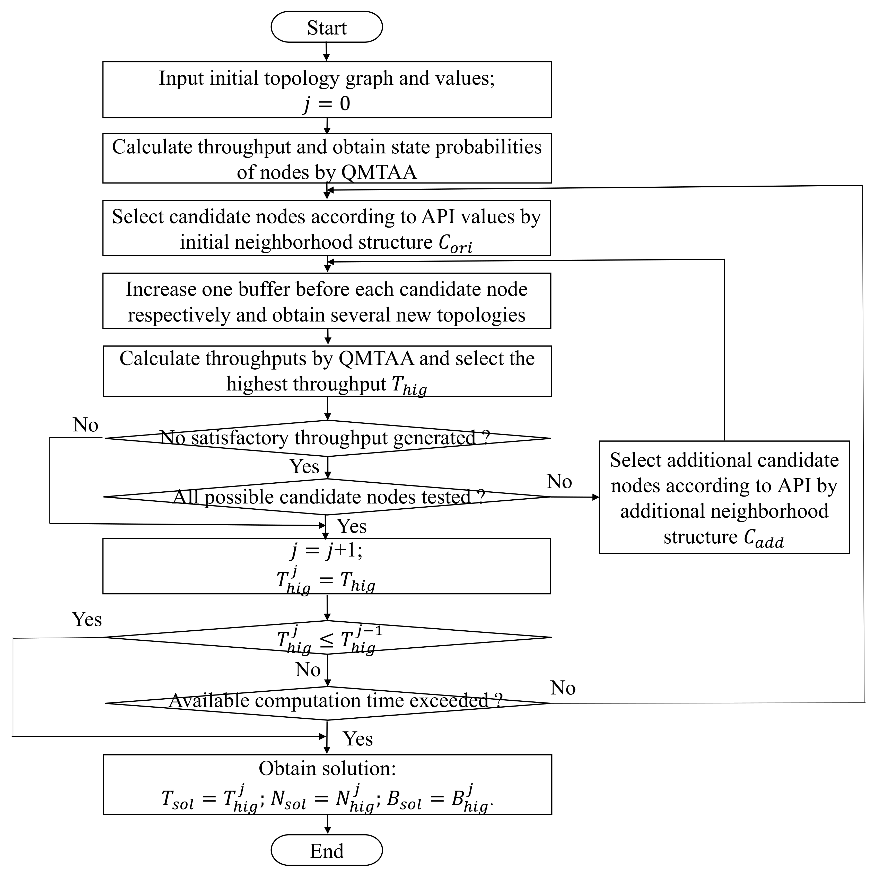
3. Solution Methodology
| Algorithm 1: bottleneck-based variable neighborhood search algorithm |
| 1 Initialize parameters |
| 2 |
| 3 at merging or splitting node i |
| 4 |
| 5 |
| 6 |
| 7 |
| 8 |
| 9 |
| 10 |
| 11 |
| 12 |
| 13 |
| 14 |
| 15 |
| 16 |
| 17 Add one buffer before one candidate bottleneck based on βi from high value to low value and generate new |
| 18 Calculate throughput of the new by QMTAA and put it into throughput set thr |
| 19 |
| 20 |
| 21 |
| 22 |
| 23 |
| 24 |
| 25 |
| 26 Add one buffer before one candidate bottleneck based on βi from high value to low value and generate new |
| 27 Calculate throughput of the new by QMTAA and put it into throughput set thr |
| 28 |
| 29 |
| 30 |
| 31 end while |
| 32 |
| 33 |
| 34 |
| 35 |
| 36 |
3.1. Notations
- : A node that models a server or buffer.
- : Number of jobs at node .
- : Steady-state probability of jobs being at node .
- : External Poisson arrival rate at node ; i.e., the average number of jobs that enter a production line from node per unit time.
- : Exponential mean service rate at node ; i.e., the average number of jobs that leave node per unit time.
- : Number of buffer updates.
- : Throughput at which jobs leave node per unit time.
- : Temporary highest throughput rate.
- : Obtained highest throughput rate at th buffer update.
- : Throughput in the solution.
- : Buffer size corresponding to the obtained highest throughput rate at th buffer update.
- : Buffer size in the solution.
- : Buffer configuration vector corresponding to the obtained highest throughput rate at the th buffer update.
- : Buffer configuration vector in the solution.
- : Search times of the initial neighborhood.
- : Search times of an additional neighborhood.
- : Number of nodes that may be the bottleneck.
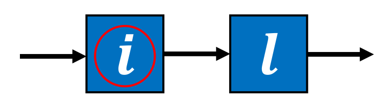
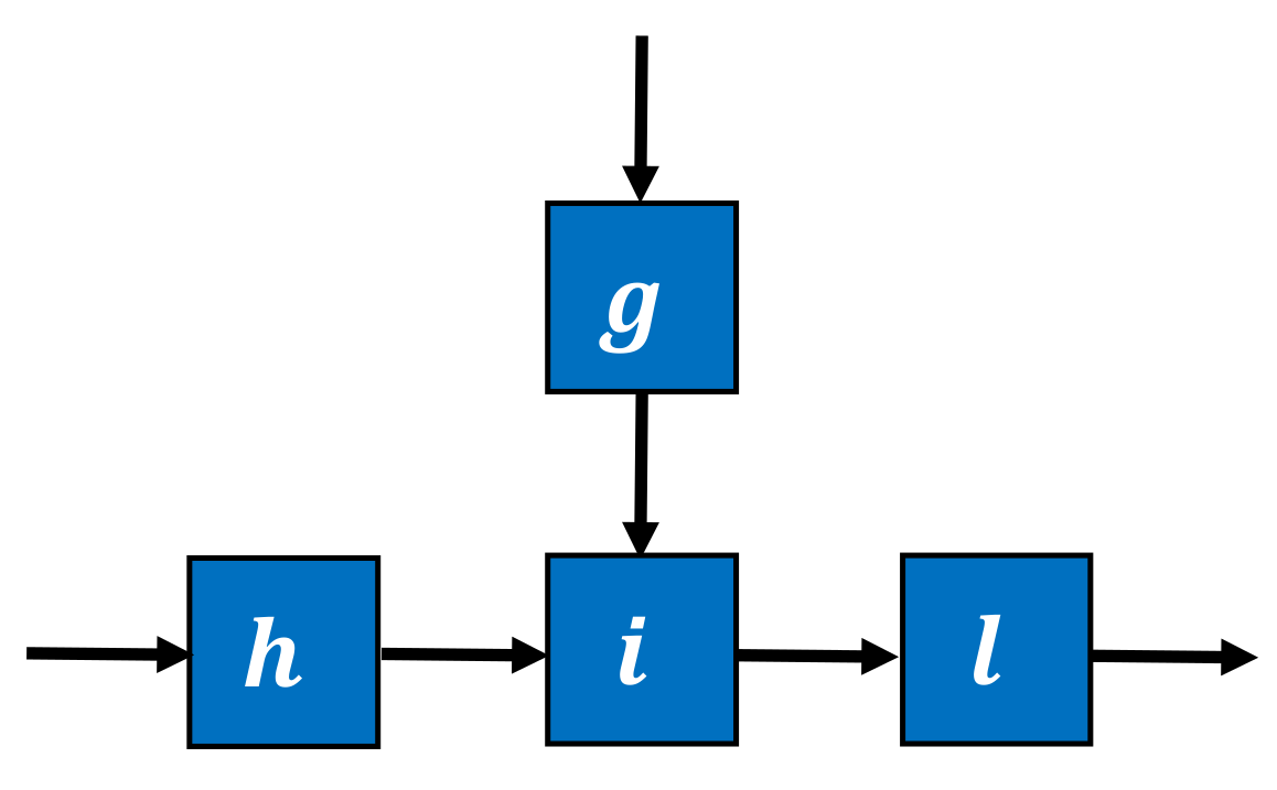
- : Number of merging nodes.
- : Number of splitting nodes.
- : Active probability index.
3.2. Queue Module-Based Throughput Analysis Approach (QMTAA)
3.3. Active Probability Index (API)
3.4. Variable Neighborhood Search (VNS)
3.4.1. Initial Neighborhood Structure
3.4.2. Neighborhood Change Criterion
3.4.3. Additional Neighborhood Structure
4. Numerical Example
- The proposed buffer allocation approach that generates candidate bottlenecks by the API and detects the real bottleneck by VNS, which is denoted by API-VNS.
- Park [24] used inventory to evaluate the candidate bottlenecks of a production line and used the beam search (BS) algorithm to search for the real bottleneck. Therefore, the inventory-based beam search algorithm (Inv-BS) is used as another method for comparison.
- Lutz et al. [28] and Papadopoulos et al. [29] used the tabu search (TS) algorithm to obtain suitable buffer allocation solutions. The solution quality of this method was shown to be high, and the computation time was controllable. Therefore, TS is used as a method for comparison. However, in prior studies, TS was typically used to maximize the throughput of a production line subject to a fixed number of designed buffers, whereas the designed buffer size is decided by available computation time in the proposed approach. For the comparison, it is assumed that in each buffer update, one buffer is added and the TS attempts to maximize the throughput. If the obtained throughput does not increase even when buffers are added, or available computation time is exceeded, the buffer allocation process stops. Otherwise, the loop of one buffer addition and throughput calculation is performed. This extended tabu search algorithm is denoted by ETS. Moreover, in the numerical examples, a random mechanism is used to generate candidate buffer allocation solutions in ETS; therefore, the average values based on five calculations are used.
- To further evaluate the effectiveness of the API, the API-BS generated by BS [24] and the proposed API is set as the fourth method for comparison.
- To evaluate the effectiveness of VNS further, Inv-VNS generated by inventory [24] and the proposed VNS is set as the fifth method for comparison.
- Solution quality refers to the obtained solution throughput because a buffer allocation approach with a high solution quality usually generates a high solution throughput. In the case of the same solution throughput, the buffer allocation approach that generates the same throughput with fewer designed buffer sizes has a higher solution quality.
- Computation time refers to the computation time spent to achieve the same throughput, because an efficient buffer allocation can allocate buffers and achieve an objective throughput rapidly.
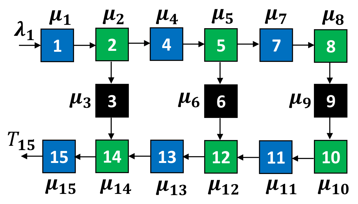
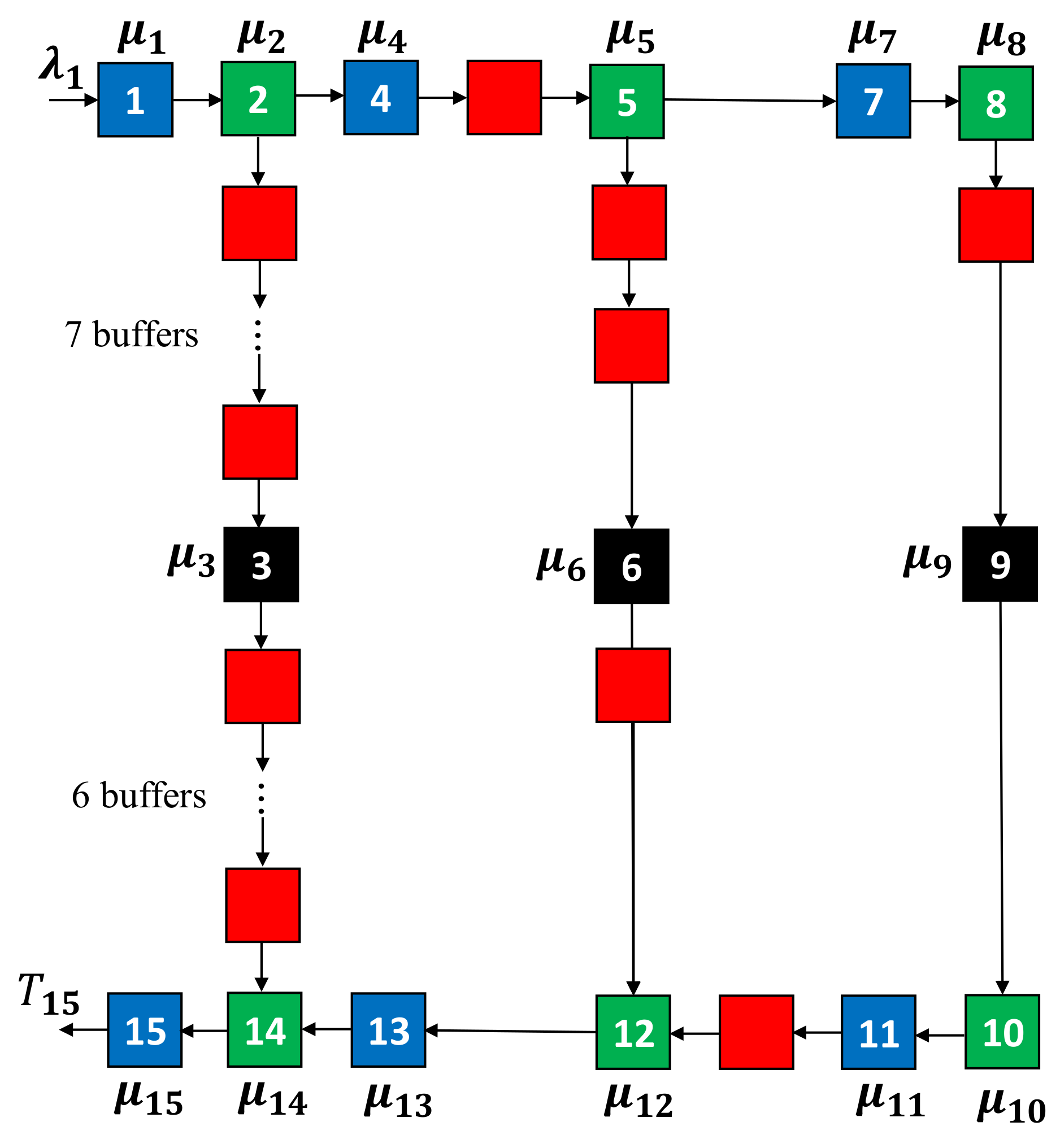
4.1. Small-Scale Topology Experiment
4.1.1. Setting
4.1.2. Results
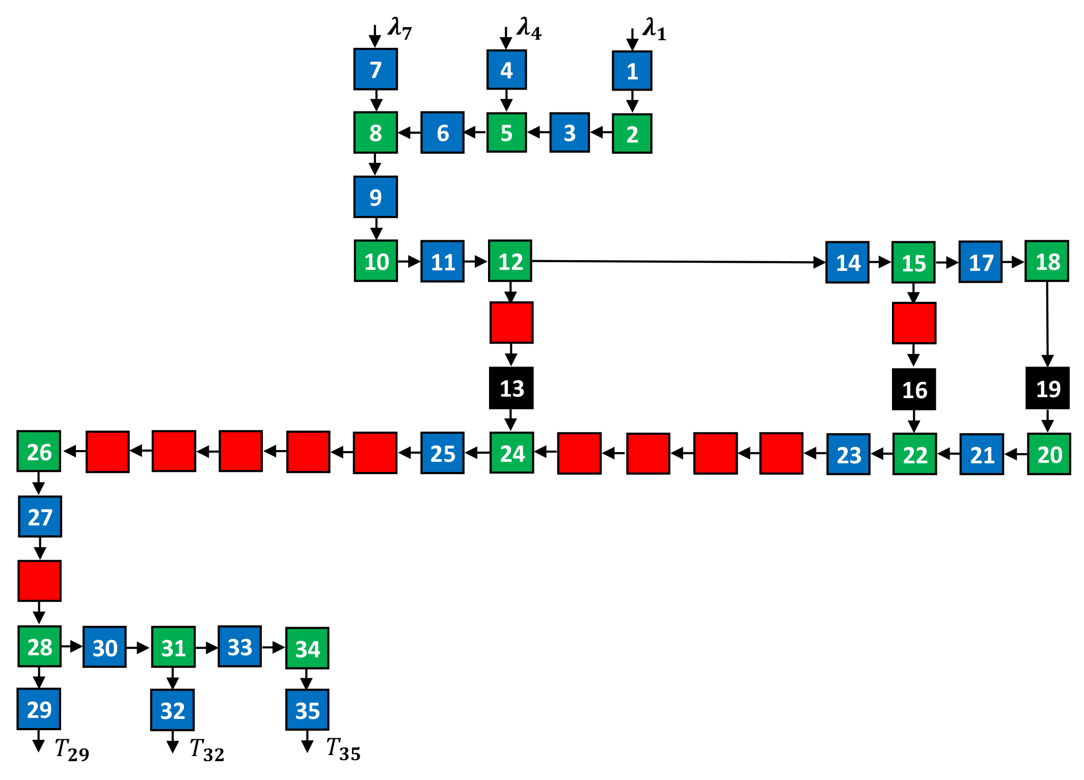
4.2. Large-Scale Topology Experiment
4.2.1. Setting
4.2.2. Results
4.3. Discussion
5. Conclusions and Future Work
Author Contributions
Funding
Conflicts of Interest
References
- Gunasekaran, A. Agile Manufacturing: A Framework for Research and Development. Int. J. Prod. Econ. 1999. [Google Scholar] [CrossRef]
- Altiok, T.; Stidham, S. The Allocation of Interstage Buffer Capacities in Production Lines. IIE Trans. 1983. [Google Scholar] [CrossRef]
- Jafari, M.A.; Shanthikumar, J.G. Determination of Optimal Buffer Storage Capacities and Optimal Allocation in Multistage Automatic Transfer Lines. IIE Trans. 1989. [Google Scholar] [CrossRef]
- Tempelmeier, H. Practical Considerations in the Optimization of Flow Production Systems. Int. J. Prod. Res. 2003. [Google Scholar] [CrossRef]
- Weiss, S.; Schwarz, J.A.; Stolletz, R. The Buffer Allocation Problem in Production Lines: Formulations, Solution Methods, and Instances. IISE Trans. 2019. [Google Scholar] [CrossRef]
- Smith, J.M.; Cruz, F.R.B.; Van Woensel, T. Topological Network Design of General, Finite, Multi-Server Queueing Networks. Eur. J. Oper. Res. 2010. [Google Scholar] [CrossRef]
- Huang, M.-G.; Chang, P.-L.; Chou, Y.-C. Buffer Allocation in Flow-Shop-Type Production Systems with General Arrival and Service Patterns. Comput. Oper. Res. 2002. [Google Scholar] [CrossRef]
- Hillier, M.S. Characterizing the Optimal Allocation of Storage Space in Production Line Systems with Variable Processing Times. IIE Trans. 2000. [Google Scholar] [CrossRef]
- Sennott, L.I. Stochastic Dynamic Programming and the Control of Queueing Systems; John Wiley & Sons, Inc.: Hoboken, NJ, USA, 2008. [Google Scholar]
- Diamantidis, A.C.; Papadopoulos, C.T. A Dynamic Programming Algorithm for the Buffer Allocation Problem in Homogeneous Asymptotically Reliable Serial Production Lines. Math. Probl. Eng. 2004. [Google Scholar] [CrossRef]
- Sadr, J.; Malhame, R. Decomposition/Aggregation-Based Dynamic Programming Optimization of Partially Homogeneous Unreliable Transfer Lines. IEEE Trans. Autom. Contr. 2004. [Google Scholar] [CrossRef]
- Kose, S.Y.; Kilincci, O. A Multi-Objective Hybrid Evolutionary Approach for Buffer Allocation in Open Serial Production Lines. J. Intell. Manuf. 2020. [Google Scholar] [CrossRef]
- Costa, A.; Alfieri, A.; Matta, A.; Fichera, S. A Parallel Tabu Search for Solving the Primal Buffer Allocation Problem in Serial Production Systems. Comput. Oper. Res. 2015. [Google Scholar] [CrossRef]
- Beşikçi, E.B.; Arslan, O.; Turan, O.; Ölçer, A.I. An Artificial Neural Network Based Decision Support System for Energy Efficient Ship Operations. Comput. Oper. Res. 2016. [Google Scholar] [CrossRef]
- Lin, J.T.; Chiu, C.-C. A Hybrid Particle Swarm Optimization with Local Search for Stochastic Resource Allocation Problem. J. Intell. Manuf. 2018. [Google Scholar] [CrossRef]
- Lin, J.T.; Chiu, C.-C. A Segmentation Approach for Solving Buffer Allocation Problems in Large Production Systems. Int. J. Prod. Res. 2016. [Google Scholar] [CrossRef]
- Li, J. Continuous Improvement at Toyota Manufacturing Plant: Applications of Production Systems Engineering Methods. Int. J. Prod. Res. 2013. [Google Scholar] [CrossRef]
- Vergara, H.A.; Kim, D.S. A New Method for the Placement of Buffers in Serial Production Lines. Int. J. Prod. Res. 2009. [Google Scholar] [CrossRef]
- Seo, D.-W.; Lee, H. Stationary Waiting Times in m-Node Tandem Queues with Production Blocking. IEEE Trans. Autom. Control 2011. [Google Scholar] [CrossRef]
- MacGregor Smith, J. Joint Optimisation of Buffers and Network Population for Closed Finite Queueing Systems. Int. J. Prod. Res. 2016. [Google Scholar] [CrossRef]
- Balsamo, S. Queueing Networks with Blocking: Analysis, Solution Algorithms and Properties. In Network Performance Engineering. Lecture Notes in Computer Science; Kouvatsos, D.D., Ed.; Springer: Berlin, Germany, 2011. [Google Scholar]
- Gershwin, S.B.; Schor, J.E. Efficient Algorithms for Buffer Space Allocation. Ann. Oper. Res. 2000. [Google Scholar] [CrossRef]
- Gao, S.; Rubrico, J.I.U.; Higashi, T.; Kobayashi, T.; Taneda, K.; Ota, J. Efficient Throughput Analysis of Production Lines Based on Modular Queues. IEEE Access 2019. [Google Scholar] [CrossRef]
- Park, T. A Two-Phase Heuristic Algorithm for Determining Buffer Sizes of Production Lines. Int. J. Prod. Res. 1993. [Google Scholar] [CrossRef]
- Roser, C.; Nakano, M.; Tanaka, M. A practical bottleneck detection method. In Proceedings of the Winter Simulation Conference Proceedings, Arlington, VA, USA, 9–12 December 2001. [Google Scholar] [CrossRef]
- Demir, L.; Tunalı, S.; Eliiyi, D.T. An adaptive tabu search approach for buffer allocation problem in unreliable non-homogenous production lines. Comput. Oper. Res. 2012. [Google Scholar] [CrossRef]
- Suri, R. An Overview of Evaluative Models for Flexible Manufacturing Systems. Ann. Oper. Res. 1985. [Google Scholar] [CrossRef]
- Lutz, C.M.; Davis, K.R.; Sun, M. Determining Buffer Location and Size in Production Lines Using Tabu Search. Eur. J. Oper. Res. 1998. [Google Scholar] [CrossRef]
- Papadopoulos, C.T.; O’Kelly, M.E.J.; Tsadiras, A.K. A DSS for the Buffer Allocation of Production Lines Based on a Comparative Evaluation of a Set of Search Algorithms. Int. J. Prod. Res. 2013. [Google Scholar] [CrossRef]


| Neighborhood Definition | ||||
|---|---|---|---|---|
| API | Inventory [24] | Random | ||
| Search algorithms | VNS | API-VNS (Proposed approach) | Inv-VNS | |
| BS [24] | API-BS | Inv-BS | ||
| TS [29] | ETS | |||
| Items | Parameters |
|---|---|
| Arrival rates | (jobs/s) |
| Service rates of buffers 1, 4, 7, 11, 13, 15 | (jobs/s) |
| Service rates of buffers 2, 5, 8, 10, 12, 14 | (jobs/s) |
| Service rates of servers 3, 6, 9 | (jobs/s) |
| Service discipline of merging | First come, first served: jobs arriving at the merging node enter it first preemptively. |
| Service discipline of splitting | Random: jobs at the splitting node move to ensuing nodes randomly. |
| Algorithm | |||||
|---|---|---|---|---|---|
| (0.4, 1.0, 0.5, 0.2) | API-VNS | 1012 | 0.2403 | 13 | (10,2,1,0,0,0,0,0,0,0,0) |
| Inv-BS | 1605 | 0.2200 | 10 | (1,0,0,2,0,1,0,3,0,3,0) | |
| ETS | Average: 14,400 | Average: | Average: | ||
| 0.2438 | 12 | ||||
| ① 0.2408 | ① 11 | ① (6,1,1,1,1,1,0,0,0,0,0) | |||
| ② 0.2492 | ② 10 | ② (4,0,4,0,1,0,0,0,1,0,0) | |||
| ③ 0.2413 | ③ 15 | ③ (11,1,1,0,1,0,0,0,0,0,0) | |||
| ④ 0.2459 | ④ 10 | ④ (5,0,2,0,2,0,0,0,0,1,0) | |||
| ⑤ 0.2416 | ⑤ 13 | ⑤ (8,2,1,0,1,1,0,0,0,0,0) | |||
| API-BS | 1476 | 0.2403 | 13 | (10,2,1,0,0,0,0,0,0,0,0) | |
| Inv-VNS | 1895 | 0.2200 | 10 | (1,0,0,2,0,1,0,3,0,3,0) | |
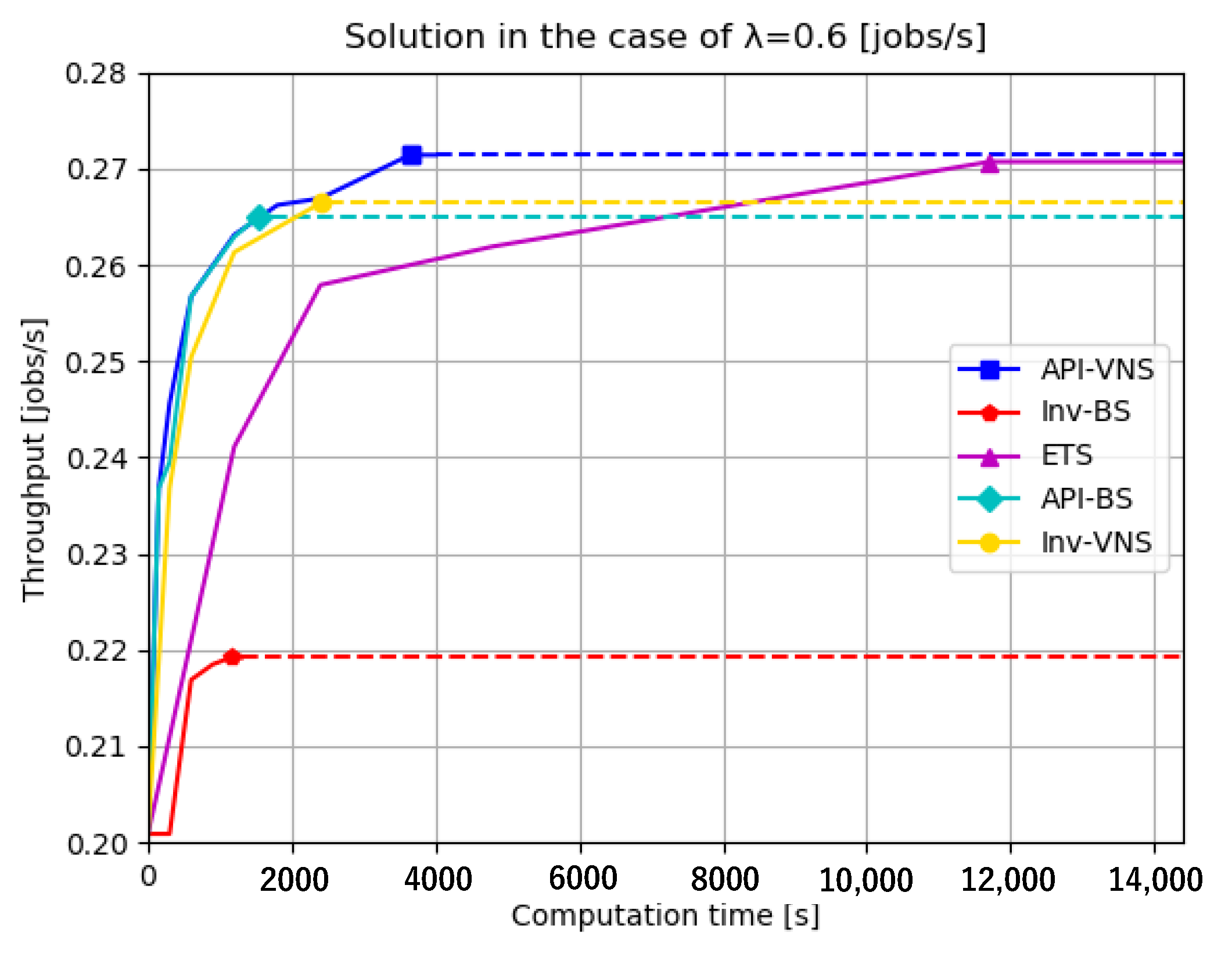
| (0.6, 1.0, 0.5, 0.2) | API-VNS | 3644 | 0.2714 | 19 | (0,7,6,1,2,1,0,1,0,1,0) |
| Inv-BS | 1148 | 0.2192 | 8 | (0,0,0,0,3,4,0,0,0,1,0) | |
| ETS | Average: 14,400 | Average: | Average: | ||
| 0.2707 | 15 | ||||
| ① 0.2714 | ① 12 | ① (0,5,5,0,1,0,0,0,0,1,0) | |||
| ② 0.2695 | ② 12 | ② (0,2,5,0,2,0,0,0,2,1,0) | |||
| ③ 0.2733 | ③ 20 | ③ (4,5,9,0,1,0,0,0,1,0,0) | |||
| ④ 0.2687 | ④ 15 | ④ (0,4,4,2,0,3,1,0,0,1,0) | |||
| ⑤ 0.2704 | ⑤ 16 | ⑤ (0,4,5,3,1,2,0,0,1,0,0) | |||
| API-BS | 1530 | 0.2650 | 14 | (0,7,7,0,0,0,0,0,0,0,0) | |
| Inv-VNS | 2399 | 0.2664 | 18 | (1,7,5,1,1,1,0,0,0,0,2) |
| Items | Parameters |
|---|---|
| Arrival rates | (jobs/s) |
| Service rates of buffers 1, 3, , 33, 35 | (jobs/s) |
| Service rates of buffers 2, 5, , 31, 34 | (jobs/s) |
| Service rates of servers 13, 16, 19 | (jobs/s) |
| Service discipline of merging | First come, first served: jobs arriving at the merging node enter it first preemptively. |
| Service discipline of splitting | Random: jobs at the splitting node move to ensuing nodes randomly. |
| Algorithm | |||||
|---|---|---|---|---|---|
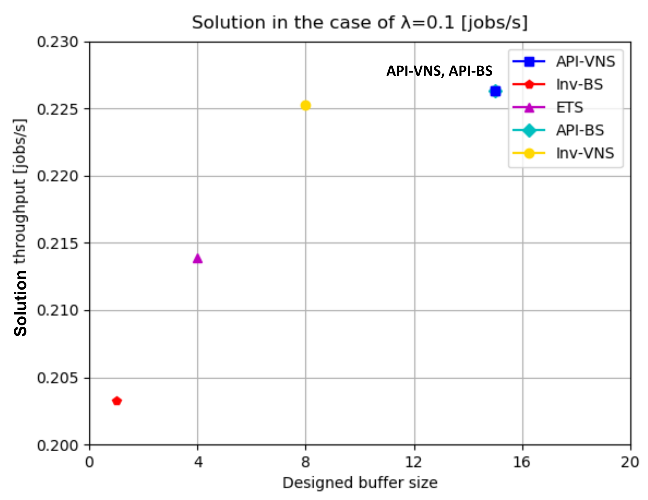
| (0.1, 1.0, 0.5, 0.2) | API-VNS | 21,430 | 0.2263 | 15 | (0,0,0,0,0,0,0,2,0,0,0,1,0,0,0,0,1,9,2,0,0) |
| Inv-BS | 633 | 0.2033 | 1 | (0,0,0,0,1,0,0,0,0,0,0,0,0,0,0,0,0,0,0,0,0) | |
| ETS | Average: 28,800 | Average: | Average: | ||
| 0.2139 | 4 | ||||
| ① 0.2154 | ① 5 | ① (0,0,0,0,0,0,0,1,0,0,0,0,0 ,0,0,1,2,1,0,0,0) | |||
| ② 0.2103 | ② 3 | ② (0,0,0,0,0,0,0,1,0,0,0,1,0 ,0,0,0,0,1,0,0,0) | |||
| ③ 0.2255 | ③ 4 | ③ (0,0,0,0,0,0,0,0,0,0,0,1,0 ,0,0,1,0,0,0,0,2) | |||
| ④ 0.2097 | ④ 3 | ④ (0,0,0,0,0,0,0,1,0,0,0,1,0 ,0,0,0,0,1,0,0,0) | |||
| ⑤ 0.2089 | ⑤ 3 | ⑤ (0,0,0,0,0,0,0,1,0,0,0,0,0 ,0,0,0,0,1,1,0,0) | |||
| API-BS | 18376 | 0.2263 | 15 | (0,0,0,0,0,0,0,2,0,0,0,1,0,0,0,0,1,9,2,0,0) | |
| Inv-VNS | 15518 | 0.2253 | 8 | (2,0,0,0,2,0,0,2,0,1,1,0,0,0,0,0,0,0,0,0,0) | |
| (0.2, 1.0, 0.5, 0.2) | API-VNS | 23924 | 0.2292 | 12 | (0,0,0,0,0,0,0,1,0,0,0,1,0,0,0,0,4,5,1,0,0) |
| Inv-BS | 745 | 0.2033 | 1 | (0,0,0,0,1,0,0,0,0,0,0,0,0,0,0,0,0,0,0,0,0) | |
| ETS | Average: 28,800 | Average: | Average: | ||
| 0.2210 | 7 | ||||
| ① 0.2275 | ① 4 | ① (0,0,0,0,0,0,0,1,0,0,0,0,0 ,0,1,1,0,0,0,1,0) | |||
| ② 0.2135 | ② 4 | ② (0,0,0,0,0,0,0,1,0,0,0,1,0 ,0,0,0,1,1,0,0,0) | |||
| ③ 0.2135 | ③ 9 | ③ (0,0,1,3,1,0,0,0,0,0,1,0,0 ,0,0,0,1,1,1,0,0) | |||
| ④ 0.2248 | ④ 8 | ④ (3,0,0,1,0,1,0,0,0,0,0,0,0 ,0,1,0,0,0,0,1,1) | |||
| ⑤ 0.2262 | ⑤ 9 | ⑤ (4,0,0,1,0,0,0,0,0,0,0,0,0 ,0,0,1,0,0,0,2,1) | |||
| API-BS | 22,371 | 0.2292 | 12 | (0,0,0,0,0,0,0,1,0,0,0,1,0,0,0,0,4,5,1,0,0) | |
| Inv-VNS | 21,884 | 0.2248 | 10 | (0,0,0,0,2,0,0,6,0,1,1,0,0,0,0,0,0,0,0,0,0) |
Publisher’s Note: MDPI stays neutral with regard to jurisdictional claims in published maps and institutional affiliations. |
© 2020 by the authors. Licensee MDPI, Basel, Switzerland. This article is an open access article distributed under the terms and conditions of the Creative Commons Attribution (CC BY) license (http://creativecommons.org/licenses/by/4.0/).
Share and Cite
Gao, S.; Higashi, T.; Kobayashi, T.; Taneda, K.; Rubrico, J.I.U.; Ota, J. Buffer Allocation via Bottleneck-Based Variable Neighborhood Search. Appl. Sci. 2020, 10, 8569. https://doi.org/10.3390/app10238569
Gao S, Higashi T, Kobayashi T, Taneda K, Rubrico JIU, Ota J. Buffer Allocation via Bottleneck-Based Variable Neighborhood Search. Applied Sciences. 2020; 10(23):8569. https://doi.org/10.3390/app10238569
Chicago/Turabian StyleGao, Sixiao, Toshimitsu Higashi, Toyokazu Kobayashi, Kosuke Taneda, Jose I. U. Rubrico, and Jun Ota. 2020. "Buffer Allocation via Bottleneck-Based Variable Neighborhood Search" Applied Sciences 10, no. 23: 8569. https://doi.org/10.3390/app10238569
APA StyleGao, S., Higashi, T., Kobayashi, T., Taneda, K., Rubrico, J. I. U., & Ota, J. (2020). Buffer Allocation via Bottleneck-Based Variable Neighborhood Search. Applied Sciences, 10(23), 8569. https://doi.org/10.3390/app10238569