Two-Layer-Graph Clustering for Real-Time 3D LiDAR Point Cloud Segmentation

Abstract

The perception system has become a topic of great importance for autonomous vehicles, as high accuracy and real-time performance can ensure safety in complex urban scenarios. Clustering is a fundamental step for parsing point cloud due to the extensive input data (over 100,000 points) of a wide variety of complex objects. It is still challenging to achieve high precision real-time performance with limited vehicle-mounted computing resources, which need to balance the accuracy and processing time. We propose a method based on a Two-Layer-Graph (TLG) structure, which can be applied in a real autonomous vehicle under urban scenarios. TLG can describe the point clouds hierarchically, we use a range graph to represent point clouds and a set graph for point cloud sets, which reduce both processing time and memory consumption. In the range graph, Euclidean distance and the angle of the sensor position with two adjacent vectors (calculated from continuing points to different direction) are used as the segmentation standard, which use the local concave features to distinguish different objects close to each other. In the set graph, we use the start and end position to express the whole set of continuous points concisely, and an improved Breadth-First-Search (BFS) algorithm is designed to update categories of point cloud sets between different channels. This method is evaluated on real vehicles and major datasets. The results show that TLG succeeds in providing a real-time performance (less than 20 ms per frame), and a high segmentation accuracy rate (93.64%) for traffic objects in the road of urban scenarios.

1. Introduction

With the rapid development of autonomous vehicle technology in the past decade, the performance of the sensors and the perception algorithm have been greatly improved. The perception system is the first stage of the autonomous vehicle system to process data. In order to ensure the vehicles’ safety when they are running at a high speed, it is generally required to complete all sensing tasks within 100 ms [1]. Furthermore, the accurate performance of perception ensures that the vehicle decision system operates correctly, which is crucial for autonomous vehicle safety [2].

3D LiDAR sensors have been applied more and more for robotics and autonomous vehicles in recent years [3]. Compared with the digital image, LiDAR has specific characteristics, such as high measurement accuracy and insensitiveness for different light conditions; it can work in both the day and the night. Considering common in-vehicle LiDAR data has a large amount of information, there are often more than 100,000 points in one frame, and it can acquire the data at a fast speed. Therefore, it is the most popular sensor in the autonomous vehicle research currently, and how to deal with such massive data has become an essential topic in the perception system [4,5]. A city environment is complex for autonomous vehicles due to a large number of traffic objects. Segmentation is an effective way to deal with this kind of cluttered point cloud, and unsupervised segmentation is instrumental in dealing with a 3D point cloud of a real scenario [6].

Point cloud clustering is the process of dividing indistinguishable points into different categories according to objects’ characters. Clustering is crucial since it reduces the amount of data at the level of 100,000 to hundreds, which can facilitate the systems ability for object detection and target tracking [7]. In point cloud clustering, the accuracy and running time are the key indicators of the system; the high-accuracy of the segmentation can reduce errors in the informed decision of the autonomous vehicle, and real-time performance enables vehicles to respond quickly in complex traffic environments, which can improve the safety of autonomous vehicles.

For dealing with the point cloud data, a method was proposed by Sebastian Thrun [8] to put the point cloud data into a certain size grid. He separates the ground by calculating the height difference of the point cloud in the grid. This method creatively uses a grid map to process the point cloud, which significantly improves the speed and makes an important contribution to the development of automatic driving technology. Michael Himmelsbach [9] proposes a polar grid method, which divides the point cloud data into different sectors and extracts the point cloud in the sector to fit and segment the point cloud in line with certain line characteristics. His method can reduce the dimensions of a point cloud to a grid map, which improves the operation speed. Lu [10] uses Gaussian distribution to cluster different objects on a grid map. The methods mentioned above are representative of the grid map method. Xu [11] uses a voxel and graph-based strategy to reduce point cloud density, and Jeremie [12] also reduces the number of regions by voxel. Although this kind of method can significantly reduce the running time, the accuracy of the results depends on the grid or voxel accuracy, and there are a lot of blank areas in the grid map, which waste space.

Bogoslavskyi [13] proposed a clustering algorithm based on a range graph. The method uses the angle on the vertical channel to segment the ground, calculates the change of vector between the adjacent point cloud, and then carries out the Breadth-First-Search in four neighbor areas to cluster the non-ground point cloud. Zermas [14] proposed a new method to utilize some seed points and two thresholds to estimate the ground fitting equation, calculate the distance from points to the fitting equation and get the result of the ground points and non-ground points. Patrick Burger proposed a mesh-graph based clustering. It traverses the point cloud from different directions, integrates multiple features as the evaluation criteria, and uses the structured neighborhood relationship between point clouds to improve the operation efficiency [15,16]. These methods have made a lot of contributions to the point cloud storage structure. The use of a graph structure [17,18] enables the vast data to represent the relationship between different points and make full use of the storage space. However, the segmentation standard designed by the above methods is relatively simple, and in some cases, over-segmentation occurs.

Bertrand Douillard [19] directly clusters all point clouds. They can use specially designed features to deal with complex point cloud scenes effectively. RANSAC is a classic method, and many point cloud clustering is improved based on this method; Adam [20] used H-RANSAC combining 2d and 3d data, Xu [21] used a weighted RANSAC for building roof plane segmentation of point clouds, and Li [22] used an improved RANSAC based on normal distribution transformation cells. Weinmann [23] used the designed 2D and 3D features to analyze the point clouds. Hu [24] used the graph model and data-driven method to cluster the point cloud. The region growing method [25,26,27], model fitting method [28,29], and hierarchical clustering method [30,31,32] are also widely used in point cloud clustering. The method of multi feature fusion is also a mainstream research direction [33,34,35]. Nevertheless, most of those methods require dense point clouds and complex mathematical models, which have a negative impact on real-time performance.

All the methods mentioned above are those popularly used at present. The grid map can significantly reduce the amount of data to be processed, and the mature image processing algorithm is applied. However, this kind of method loses the accuracy of clustering results. The second kind of method uses the range graph to simplify the storage, but there are some over-segmentation problems. The third method ensures the accuracy by designing features and models; however, the calculation process is complex, and the running time is long. Some single frame processing methods can reach more than 1 s, which is unacceptable for the real-time system. For a real-time system, the implementation of the whole perception system needs to be controlled within 100 ms [1]. At the same time, the accuracy of clustering results is related to the subsequent recognition task. It is necessary to ensure that more than 85% of a point cloud of a particular object can be correctly classified, and the running time of some excellent methods can be less than 40 ms [13,16,36].

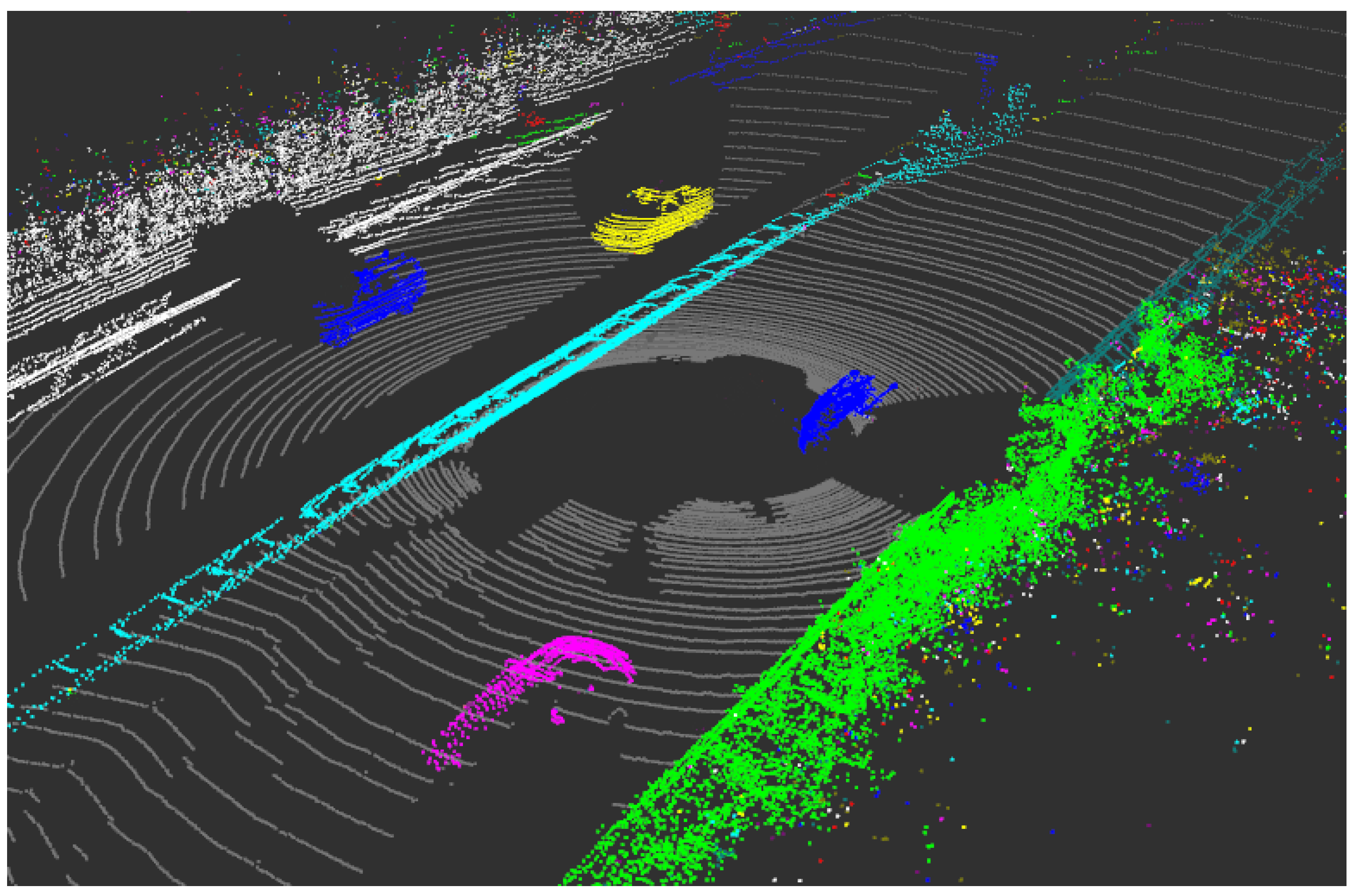
In order to meet the real-time and accuracy requirements of autonomous vehicles, we design a Two-Layer-Graph clustering method (improved from the range graph) and use an improved BFS algorithm. In Figure 1, different objects are represented by points of different colors, our method can not only ensure the accuracy but also compress the running time as much as possible. Also, particularly, we design the segmentation standard to solve this kind of over-segmentation problem.

2. Data and Problem Analysis

In this section, we will explain the characteristics of a LiDAR 3D point cloud data, some clustering strategies according to different characteristics, and some issues in the process of clustering. The analysis of these data characteristics and problems will provide help for the design of the clustering method.

2.1. LiDAR Data Characteristics

In the task of point cloud clustering, we need to be familiar with the characteristics of the point cloud collected by the LiDAR. For the rotary LiDAR, like Velodyne 64E, the main characteristics of point clouds are as follows:

(1) Sparse density in different directions: For the same object, the point cloud in the horizontal direction is dense, while the vertical direction is relatively sparse. Therefore, the processing point cloud in the horizontal and vertical directions needs different methods to adapt to its density characteristics [37]. For point clouds in the same horizontal channel, if the Euclidean distance is less than a particular threshold value, it can be regarded as the same category. However, if the distance exceeds the threshold value, other judgment methods should be added to prevent over-segmentation. For points in the same vertical direction, they come from different channels, for which we need to calculate their spatial position relationship, and the selection of the threshold is also different.

(2) Distance to the sensor: The point cloud collected at close range is dense, but the distant object only has sporadic point clouds. With the same angular resolution, the farther the distance is, the greater the distance between the same included angles is [36]. So an object’s point cloud density depends on the distance to the sensor. For the point cloud nearby, the distance between ten adjacent vertical angle units is still relatively close, while for the distant point cloud, the difference of several vertical angle units is far in space.

(3) Missing point cloud: Although the number of lasers collected from the LiDAR is same at a certain frequency, the amount of data collected by the receiver is different. The point cloud in some angles is missing, because black areas absorb laser light, or it might be sent to the sky and not return, and these missing data need to be handled properly, preventing it from interfering with clustering speed. Therefore, we need to establish a connection method, which can mark the invalid points and quickly find the effective point clouds on different sides of the invalid points.

2.2. Analysis of Clustering Tasks

The ability to run point cloud clustering in real time needs to be optimized in multiple aspects. We mainly focus on the following aspects to make our proposed clustering algorithm faster than other methods.

(1) Storage structure: The general point cloud is disordered, but the data of the rotary LiDAR has a certain organizational structure because of its collection principle. By organizing it into an orderly structure, the speed of reading is greatly improved. In addition to the storage structure of the point cloud, the data attributes of a single point are also what we need to pay attention to. How to update the attributes of each point quickly is the key to improving the speed of calculation, so it is necessary to design the storage structure of a point cloud with suitable data attributes. The range graph is useful in the presence of the neighborhood relationship of point clouds, easy to search, and will not waste storage space; this storage structure has been used in many researches [13,16]. A graph structure can effectively represent the relationship between points [38,39], and a single graph node can represent point cloud groups. According to the characteristics of the original point cloud data, we design a Two-Layer-Graph structure based on a range graph and use edges to represent their neighborhood relationship. This structure combines the advantages of a range graph (save space, easy to read and write) and graph structure (application of fast search algorithm), which dramatically improves the efficiency of the algorithm.

(2) Segmentation standard: For the original point cloud, each point has its own angle information and 3D space position information. Whether to classify different points into one category or different categories is also the focus of attention, so suitable segmentation standards are very important. Standards can affect the accuracy of the clustering results, but complex segmentation standards will consume more running time. In the face of different application requirements, we need to choose some suitable segmentation standards. The standard method is to use Euclidean distance and segments according to the distribution characteristics of continuous points or to calculate the angle relationship of adjacent point clouds [13,15], and an optimal neighborhood should be selected [40]. Considering the difference in point cloud density, we design different segmentation standards in horizontal and vertical directions. In the horizontal direction, we use the Euclidean distance and the angle between the vectors on both sides of the adjacent points and the sensor position as the segmentation standard, and the distance of the horizontal projection in the vertical direction.

(3) Category update: In the process of point cloud clustering, the category of a single point cloud or a partial area point cloud can not be determined at once. It is necessary to update the category of point cloud. The method to update the category greatly affects the real-time performance of the point cloud clustering. Patrick Burger [15] updates the categories after the initial segmentation using connection maps in different directions. It is a common practice to use a breadth-first-search algorithm in the search, which is used in many fields of automatic vehicles [13,41]. In the graph structure storage model we designed, we improved the breadth-first-search method for data characteristics.

3. Proposed Method

In this section, we propose Two-Layer-Graph (TLG) clustering method, which significantly increases the speed of calculations while ensuring the accuracy of segmentation. We divide the task of point cloud clustering into three parts: (1) storage structures, (2) segmentation standards, (3) category update.

3.1. Storage Structures

For point cloud data storage, in order to meet real-time performance, we give these requirements:

• Fast read and write: For over 100,000 pieces of point cloud data, we need to quickly locate each point cloud and be able to modify its attributes.
• Data connection: For a point cloud scene, we need to express the connection between point clouds and find the neighbor points of any point cloud quickly.

In response to the above requirements, we designed the following point cloud Two-Layer-Graph structure, the layer of range graph to save single points, and the layer of point cloud set graph to save points set.

3.1.1. Range Graph

For the entire point cloud scene, we use the range graph structure for storage. It can meet the point cloud-level traversal requirements and achieve high-speed access to any point data. The structure of the range graph is consistent in Figure 2. The length and width represent the horizontal angle and vertical angle of the point cloud, for each point cloud with a single point structure, located at the node position of the channel number and the horizontal number. Nevertheless, some node of the range graph does not have a valid point, so a valid attribute is designed in the single point storage structure.

The single point structure in

Table 1. Single point structure.

Attributes	3D Position	Angle Info	Valid	1ST LBL	FIN LBL
Symbol	x,y,z,d	Ver,Hor	V	$\alpha$	$\beta$
Uint	Meter	Integer	T/F	Integer	Integer

not only stores standard point cloud information, such as point cloud x, y, z three-dimensional information, distance information d, serial numbers in the horizontal and vertical directions, but also contains several vital attributes, such as whether it is a valid point, the category number after the first segmentation $\alpha$, and the final category $\beta$. These attributes do not come from initial data but the attribute information that needs to be processed. The design of each attribute’s information can help improve real-time performance.

Range graph can well represent the neighbor relationship of point clouds; we can find the neighbor point fast by this structure. In TLG, the range graph is the first-level graph structure. Moreover, in this graph, we do the first segmentation of the point cloud in each channel.

3.1.2. Point Cloud Set Graph:

Two processes complete the method proposed in this paper, the clustering of point clouds. The first step is a channel-level clustering process. So a structure for storing the point cloud set after the first segmentation is designed. In Figure 3, a graph node structure represents a point cloud set, and the lines connecting different nodes present the neighbor relationship of nodes. It has the same number of channels as a range graph, but in each channel, the number of graph nodes is not consistent.

Table 2. Point cloud set node.

Info	Channel	Start Pos	End Pos	LBL NO
Symbol	C	S	E	N
Uint	Integer	Integer	Integer	Integer

shows the information of a point cloud set node. Each node represents a point cloud set, contains information about start position, end position, channel number and category label in the current channel.

The set graph is the second-layer graph structure we proposed. In Figure 3, the set graph merges the point clouds that belong to the same category into one node.

A node stores the start position, end position and channel number of the point cloud set, so reading the information of a node can quickly find the corresponding point cloud set. Using nodes instead of searching each point cloud is beneficial to improve the efficiency of the second clustering processing.

3.2. Segmentation Standard

To judge whether two point clouds belong to the same category, the standard of segmentation is the key to the accuracy of results. Because of the difference in density between the vertical and horizontal directions, this paper uses a variety of features to distinguish point cloud categories.

3.2.1. Horizontal Direction

The continuous point clouds under a channel have the same vertical angle, and the horizontal angle between adjacent point clouds is very small, showing a dense feature. We perform the first segmentation operation of point clouds under the same channel. The primary standards used are distance and angle characteristics.

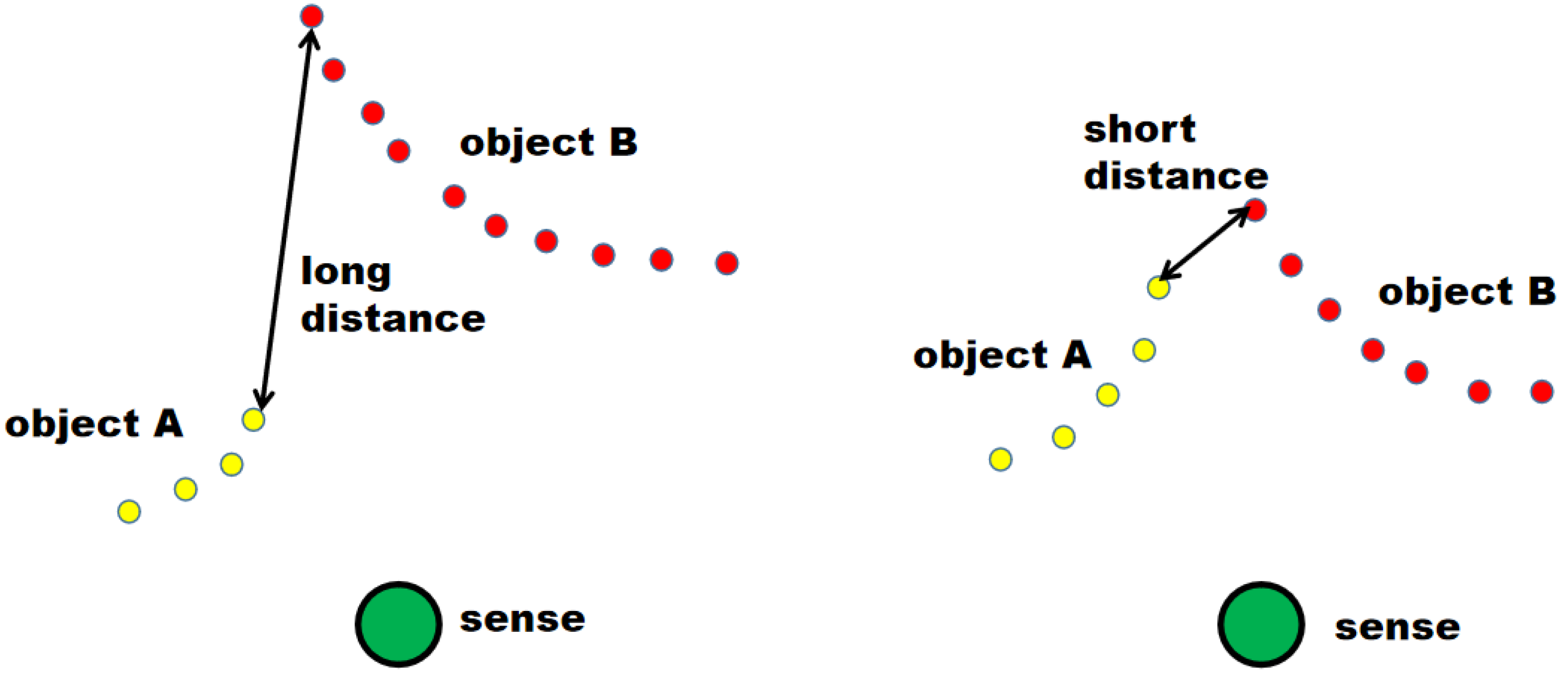
In Figure 4, some adjacent points belong to different objects under the same channel, have a long-distance difference on the horizontal plane, so distance can be used as the segmentation standard directly. So we use the distance between adjacent point clouds as one of the segmentation standards.

For two points under the same channel $ve{r}_1$:

$$p_{ver1,hor1}=\{x_1,y_1,z_1,d_1,ve{r}_1,ho{r}_1,V_1,{\alpha }_1,{\beta }_1\}$$

(1)

$$p_{ver1,hor1+1}=\{x_2,y_2,z_2,d_2,ve{r}_1,ho{r}_2,V_2,{\alpha }_2,{\beta }_2\}$$

(2)

x, y, z represent 3D space coordinates, d represents the distance from the point cloud to the sensor, $ver$ and $hor$ are the vertical angle and the horizontal angle, V represents whether the point is valid, $\alpha$, $\beta$ represent the first category label and the final category label. These two parameters are both −1, which means that the segmentation process has not been performed yet.

We first calculate the distance on the xy plane.

$$dis=\sqrt{{(x_1-x_2)}^2+{(y_1-y_2)}^2}>T{h}_{dis}$$

(3)

In the left of Figure 4, if the distance between two adjacent points is over a certain threshold, we think they belong to different categories. However, there are also some adjacent point clouds that belong to different objects with close distance in the right of Figure 4, but it is not easy to segment them using only the distance standard. For this case, we have designed an angle-dependent segmentation standard. Different from other methods, we first calculate the vector angles on different sides of the adjacent points. This method takes into account the position relationship of five points, including the sensor position, to determine whether the adjacent two points belong to the same category.

For adjacent point clouds in a short distance, we obtain the vector directions to the point clouds on different sides and then calculate the direction of the angle bisector of the two vectors.

Using $V_1$ and $V_2$ in Figure 5a to represent the unit vectors from points $p_{ver1,hor1}$ and $p_{ver1,hor1+1}$ to adjacent point clouds on different sides. Calculate the unit vector on the bisector of the angle of the two unit vectors $V_{angle-bisector}$.

$$V_{angle-bisector}=\frac{V_1+V_2}{\parallel V_1+V_2\parallel }$$

(4)

The vector from the midpoint of points $p_{ver1,hor1}$ and $p_{ver1,hor1+1}$ to the position of the sensor, we call it $V_{m-o}$:

$$V_{m-o}=(-\frac{x_1+x_2}{2},-\frac{y_1+y_2}{2})$$

(5)

$$V_{m-o}{V}_{angle-bisector}>0$$

(6)

$$arccos\left(\frac{V_1{V}_2}{\parallel V_1{V}_2\parallel }\right)<T{h}_{angle}$$

(7)

When Formulas (6) and (7) are met, the inner product of vector $V_{angle-bisector}$ and vector $V_{m-o}$ is greater than zero, and the angle between vectors $V_1$ and $V_2$ is less than the threshold $T{h}_{angle}$, the two points are divided into different categories.

If the angle bisector is located at the position enclosed by the red dashed line in Figure 5c, and the angle between $V_{angle-bisector}$ and $V_{m-o}$ is less than a certain threshold, the two adjacent points are classified into different categories. If it is located in the shadow of the black dashed area, the two points are of the same category. In this subsection, we use the local concave features to distinguish different objects close to each other with as little data as possible.

3.2.2. Vertical Direction

In the vertical direction, the work of point cloud clustering is mainly to merge different types of point cloud sets. For points belonging to different channels, we use the distance on the xy plane as the merge standard.

$$Dis=\sqrt{{(X_1-X_2)}^2+{(Y_1-Y_2)}^2}>T{h}_{Dis}$$

(8)

$X_1$, $X_2$, $Y_1$, and $Y_2$, respectively, represent the coordinate positions of point clouds belonging to different channels in the xy plane.

3.3. Category Update

A category update requires the use of a search algorithm. The search algorithm is a method of traversing the point cloud. The fewer times the point cloud is traversed, the less time it takes. We traverse the two-layer-graph structure twice according to the segmentation steps.

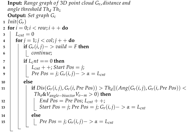
The first traversal is on the range graph. It uses the horizontal segmentation standards to divide the points under each channel into different sets. In Algorithm 1, first initialize the range graph (line 1), segment according to each channel (line 2), first set the category label to 0 (line 3), traverse in the order of the horizontal rotation angle (line 4), if it encounters an invalid point, skip and continue searching (line 5–6)in Figure 6a, If it is the first valid point of the current channel (line 7), add 1 to the category label, use the current position as the start position and Pre Pos, and mark the first label of this point on the range graph (line 8–11). If the segmentation condition is met, the current point and Pre Pos point belong to different categories, assign the end position to Pre Pos, add a node in the set graph, add 1 to the category label, and use the current position as the new start position and Pre Pos (line 13–18). If the segmentation condition is not met, Pre Pos is updated, and marks the current label for the current position (line 19–21) in Figure 6b.

Algorithm 1: First segmentation Algorithm

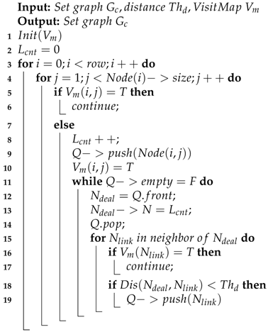
The second step is mainly to merge the graph nodes of the point sets in Figure 6c. In this step, only graph nodes under each channel are traversed. We use an improved BFS algorithm based on the neighbor relationship of the set graph.

In Algorithm 2, the visit map is initialized first (line 1), all nodes are in the unvisited state, a category label is assigned the value of 0 (line 2), and each channel is searched (line 3). If the current node has been visited in the visit map (line 5), the node is skipped (line 6). Find a node that has not been visited, add 1 to the category label, and add it to the queue. The visit map corresponding to the node is marked as visited (line 7–10). When the node queue is not empty, take the first node of the queue and mark its category as the current category label (line 11–14). Search the nodes near the current node (the nodes in upper and lower adjacent channels, which are connected to the current node and the first unconnected node on both sides, as shown in Figure 7). If the node is not visited or meets the requirements of node merging, join the node queue (line 15–19). Repeat until the queue is empty.

Algorithm 2: Set graph clustering Algorithm

Compared with BFS, not all connected nodes need to be traversed (the same channel is not traversed), and some nodes that are not connected can also be traversed (the first unconnected node on both sides of the adjacent channel).

4. Result and Discussion

We used the LiDAR data of Velodyne 64 to test a large number of data in the Ubuntu 16.04 system with Intel i5-7200u 2.5Ghz CPU and RAM 8G.

4.1. Segmentation Results Visualization

The main purpose of clustering is to distinguish the objects in traffic scenes effectively. We used the Semantic KITTI [42,43] data set to test, which is a classic data set in automatic driving, including point cloud, image, IMU and other data. Semantic Kitti is a data set with point cloud level annotation. We compare the annotation of this dataset with the experimental results and can get the accuracy of our method.

In Figure 8, two Semantic KITTI point clouds in city scenarios are shown in the form of a range graph: the precisely labeled data is the upper image, and the lower image is the result of the proposed method. The horizontal direction of the range graph represents the horizontal angle of the point cloud, and the vertical direction represents the vertical angle. Each pixel represents a point cloud, and different colors represent different categories. Among them, black indicates that the point is invalid, and no point is returned at this angle.

Compared with the accurate annotation data and the results of our proposed method, the traffic objects in the road are well distinguished, which meets the requirements of automatic driving vehicles for point cloud segmentation. The results show that the vehicles in Figure 8 are well differentiated from the surrounding environment. In the next subsection, we will show the test results on the entire Semantic KITTI dataset.

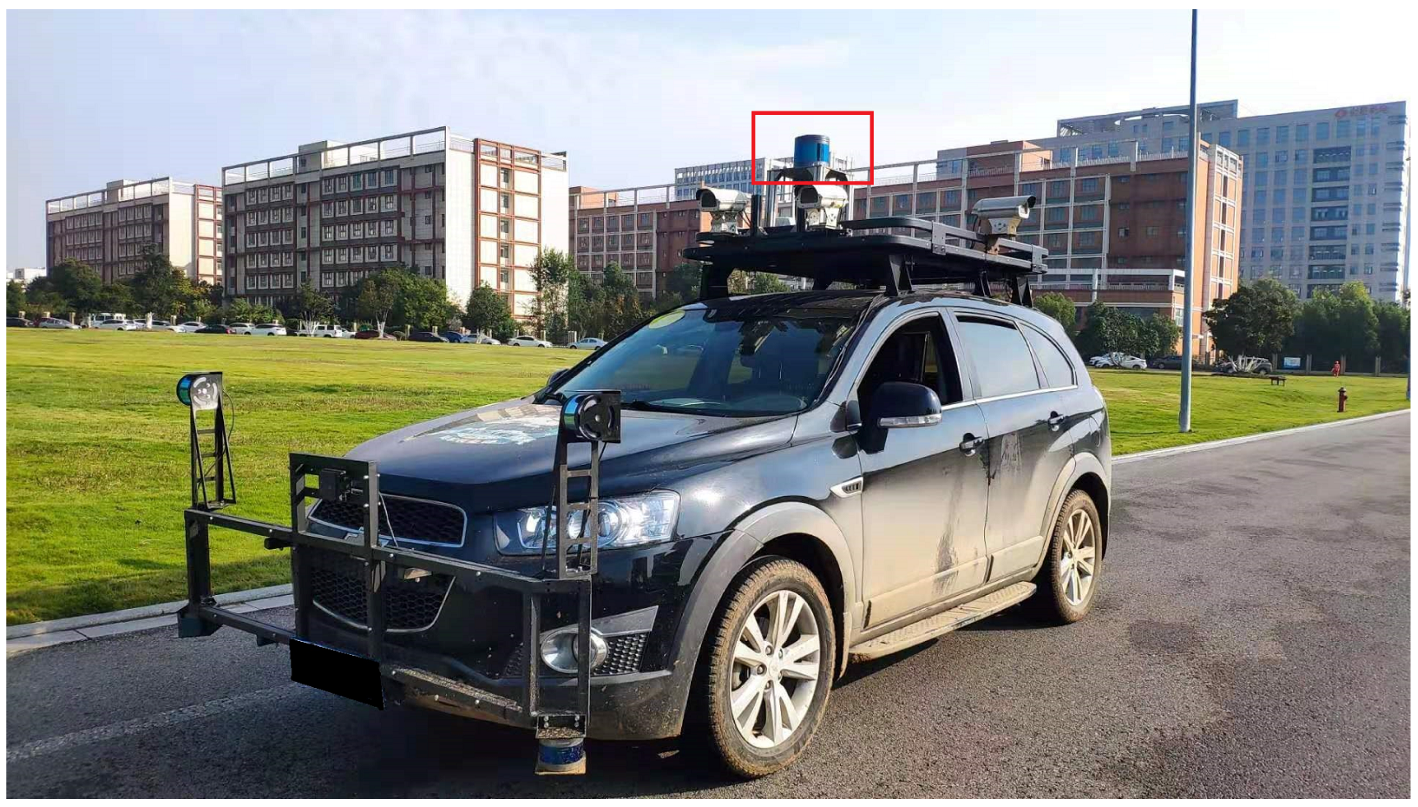
We also apply our clustering algorithm to an automatic vehicle to test the method. Figure 9 is our test platform. Robosense RS-Ruby (128 channels) LiDAR sensor is installed on the top of the car. Compared with the 64 channel LiDAR, the sensor needs to process more data per frame and has higher requirements for the real-time performance of the algorithm.

In Figure 10, we show the point cloud segmentation results of a complex traffic scene. On the road with heavy traffic, our method can well distinguish different traffic objects, which shows that the segmentation standard we adopted is very effective. The detailed perspective in Figure 10 shows that adjacent vehicles are divided into different categories. The trees outside the road are also well distinguished.

The algorithm on real vehicles needs to ensure the accuracy and real-time performance of higher standards to meet the application requirements of real vehicles. So we test the accuracy and running time of the proposed method.

4.2. Accuracy

We use the Semantic KITTI data set to test the clustering results. The main test is the accuracy of the clustering of road participants such as vehicles, motorcycles, and pedestrians, i.e., to calculate how many point clouds belonging to the same category are classified into the same category.

For a traffic object in the road, we assume that its real point cloud set is $P_{object}=\{p_1,p_2,\dots ,p_n\}$ after clustering. These points may be divided into different categories or belong to the same category. We count the largest number of categories in the set as $N_{max}$, the accuracy calculation formula of this object is as follows:

$$Ac{c}_{single}=\frac{N_{max}}{n}$$

(9)

The distance between the traffic object and the sensor is calculated as follows:

$$Di{s}_i=\sqrt{{\left(X_i\right)}^2+{\left(Y_i\right)}^2}$$

(10)

$$Di{s}_{single}=\frac{Di{s}_1+Di{s}_2+\dots +Di{s}_n}{n}$$

(11)

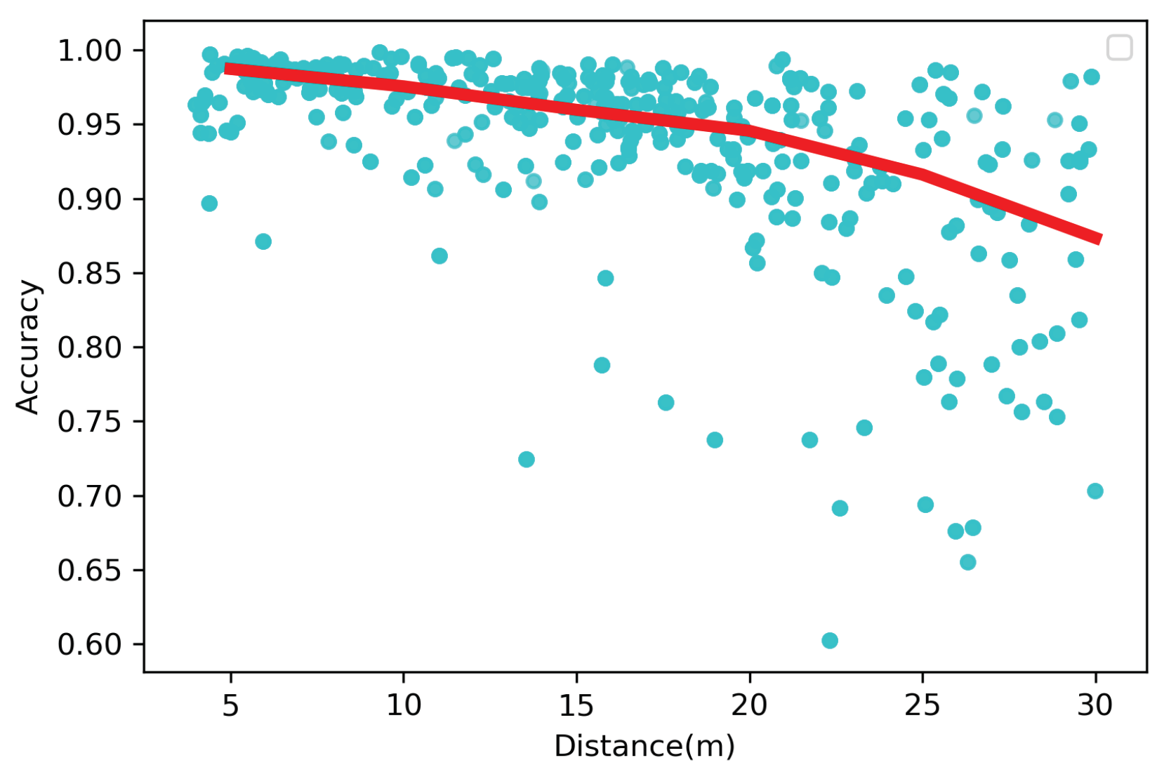
We test the relationship between object distance and accuracy, and get the result in Figure 11. The accuracy of traffic objects decreases with the increase of distance, and the accuracy of most objects remains above 90%. The red line is the curve of accuracy change at different distances.

We find that as the distance of the object increases, the accuracy will decrease. In this regard, we believe that this is because the point cloud data in the distance is very sparse and the loss of information occurs at a distance, considering the mechanism of returning to the effective point from the LiDAR. However, in the real vehicle test, we find that when the point cloud data exceeds 40 m away, the amount of data itself is very small, and the vehicle information may only have a dozen point clouds. What we really concentrate on is that on the road within 40 m, the accuracy of the method we proposed can meet the requirements.

After calculating the accuracy of a single object, we calculate the accuracy of the objects in the whole scene, and correspondingly the result is the accuracy of the traffic objects in the whole scene. If there are N objects, the accuracy in this scene is as follows:

$$Ac{c}_{scene}=\frac{n_1\ast Ac{c}_{single1}+n_2\ast Ac{c}_{single2}+\dots +n_N\ast Ac{c}_{singleN}}{N}$$

(12)

Calculate the average distance of all traffic objects in the whole scene:

$$Di{s}_{scene}=\frac{n_1\ast Di{s}_{single1}+n_2\ast Di{s}_{single2}+\dots +n_N\ast Di{s}_{singleN}}{N}$$

(13)

We compare the accuracy results of our method and several effective methods in different distances (the average distance of a scene), and found that our method has better accuracy than other methods. The average accuracy of our results is 93.64%, and the accuracy performance at different distances is shown in

Table 3. The scene accuracy of different methods at different distances.

Distance	Less 15 m	15–20 m	20–25 m	25–30 m	Over 30 m
Bogoslavskyi	0.954	0.932	0.904	0.893	0.864
Patrick Burger	0.970	0.955	0.948	0.907	0.886
Proposed	0.976	0.959	0.946	0.916	0.874

.

Bogoslavskyi’s method only uses a range graph in the horizontal direction, calculates the angle between two adjacent points and the sensor position, and uses the angle change between continuous points in the vertical direction as the segmentation standard. If the angle is larger than the threshold, points are divided into different categories. Finally, he directly updates categories by using the breadth-first-search algorithm of four neighborhoods on the range graph.

Patrick Burger designed the loss function according to the spatial distribution of multiple continuous point clouds in the horizontal and vertical directions, giving different weights to different point clouds to get two segmented maps, which are horizontal and vertical. It also updates the category by combining the connection between the two maps.

Compared with the above two methods, the main reason why our method performs well is as follows. It is more appropriate to judge whether two adjacent points belong to the same category through five critical positions. Bogoslavskyi only considers two adjacent points and sensors. Peripheral points also play a decisive role. Patrick burger uses multiple points that are continuously distributed, and too many points may also affect the results.

4.3. Running Time

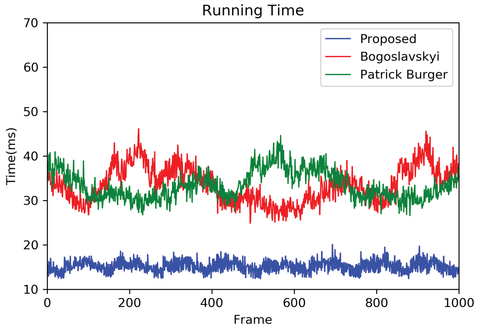
In Figure 12, we test the running time of different methods on the same platform, and we find that the average running time of some classic and effective methods (algorithm of [13,15]) is about 30–40 ms, but the average time of our proposed method is 15.53 ms. Most of the running time can be controlled within 20 ms. From the running time curve, we can infer that the stability of our algorithm performs well, and running time does not change greatly with the change of scene.

Our algorithm not only improves the segmentation standard but also reduces the running time because of the search structure. Bogoslavskyi directly uses the search algorithm on the range graph, which needs to search every point, consuming a lot of time. Burger proposes to segment in different directions, and then use two range maps to update the category. However, in the vertical direction, the relationship between each pair of adjacent points must be judged, which takes some time.

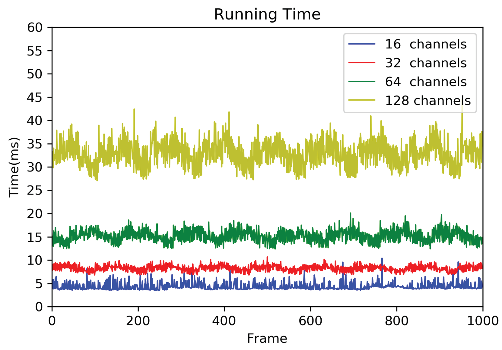
In order to better test the generality of the clustering algorithm, we test the following four different LiDARs: Robosense RS-LiDAR-16, Velodyne HDL-32E, Velodyne HDL-64E, Robosense RS-Ruby (128 channels). These LiDARs have 16, 32, 64 and 128 laser channels, respectively, and the data volume increases linearly. It can be concluded from Figure 13 that the running time of our proposed method is nearly linear with the increase of data volume. In the first traversal, the time complexity is $O\left(N\right)$, the time increases linearly with the data. The second traversal is on the set graph, the improved BFS algorithm is used, and the time complexity is $O(N+E)$. However, in the second traversal, the calculation times are related to the number of nodes and edges. In the worst case, all single points are nodes, and the time increases linearly with the amount of data. Therefore, the method we proposed is a linear algorithm; it can be used in a variety of LiDARs.

5. Conclusions

In this article, we propose a point cloud clustering algorithm with a Two-Layer-Graph structure. Through the merging of graph nodes, we get the simulation results, which show that our method has a high-quality accuracy (the accuracy rate of objects in the road is 93.64%) while the running time of our method is less than 20 ms. We test it on the actual vehicle and find that our method meets the requirements of real-time operation with different LiDARs.

The accuracy of our proposed method in segmentation performance is better than some classic methods. The possible reasons are as follows: (1) more effective selection of the vectors from adjacent points to different sides, and (2) the consideration of the relationship with the position of the sensor devices. Compared with other methods, our method, i.e., the TLG method, uses the least information to represent the characteristics of the object itself and the location relationship with the autonomous vehicle. It not only satisfies the richness of information but also saves the computing time, using the local concave features to distinguish different objects close to each other with as little information as possible.

The running time of TLG has been greatly compressed compared with other methods. The TLG clustering algorithm mainly improves the point cloud structure, segmentation standard and search algorithm. Its point cloud structure is closely related to the search algorithm, which can greatly improve the operation speed and omit some unnecessary calculations. When updating, instead of performing operations on all adjacent points in the vertical direction, it can merge in the form of nodes, which greatly improves the operating efficiency. In the worst case, its time complexity is linear. In recent years, the laser channel of LiDAR has been increased to obtain more environmental information, so the linear time complexity is very important, so that TLG clustering can do a good job. The biggest contribution of this paper is to reduce the processing time to less than 20 ms, and ensure high accuracy.

Our method also has limitations. The segmentation standard is designed for traffic objects, and we mainly evaluated the method on a large number of urban scenes. It is not tested in the complex wild environment, where there are more disordered objects on the road (weeds, shrubs, etc.) and those may affect the segmentation results.

In the promising future direction, we will consider how to use the clustering results for real-time target recognition and point cloud clustering of multiple LiDAR. In addition, we plan to introduce continuous time to help two-layer-graph point cloud clustering.