Experimental Analysis of the Dynamic Stiffness in Industrial Robots

Abstract

Industrial robots are regularly being employed for machining tasks. As a key machining parameter, dynamic stiffness has a significant influence on robotic machining performance. This paper examines two experimental approaches for obtaining the dynamic stiffness of an industrial robot. One approach is based on experimental modal analysis. The other approach is a direct calculation with the acquisition of excitation forces and vibration displacement. Different excitation frequencies are planned to stimulate an industrial robot. The dynamic stiffnesses obtained by the two approaches are thoroughly evaluated. Large deviation appears between the dynamic stiffness measured by two approaches. The factors that result in variations in the measurements are discussed.

1. Introduction

Compared to a machining center, an industrial robot has a lower stiffness value. In addition, the stiffness distribution is nonlinear within the range of the workspace. Huseyin et al. investigated the static stiffness of different robot pose configurations in a machining plane, and their results indicated that the values change in the range from $5\times {10}^{-7} \mathrm{m}/\mathrm{N}$ to $14\times {10}^{-7} \mathrm{m}/\mathrm{N}$ [1]. The stiffness value includes both the static stiffness and the dynamic stiffness. To improve machining accuracy, most studies have focused on the static stiffness of industrial robots. Through establishing stiffness models for industrial robots, the deformations resulting from the machining force can be compensated. E. Abele et al. used two approaches to obtain the cartesian stiffness of an articulated industrial robot. The first approach established a stiffness model based on virtual joint modeling (VJM). Each joint stiffness value was identified through experiments, and the Cartesian stiffness was calculated with the stiffness model. Another approach measured the Cartesian stiffness directly in the workspace. The results indicated that the calculated stiffness based on the stiffness model was nearly twice as high as the experimental stiffness. Milling tests were conducted with Aluminum AW-2017A. The calculated displacement of the robot end effector based on the experimental stiffness is almost equal to the measured displacement [2]. Zengxi Pan et al. adopted the same approach to get the static stiffness model by measuring the stiffness of an industrial robot in the workspace. This stiffness model was used for real-time deformation compensation in robotic machining. End milling was conducted with an aluminum block. With the compensation, the mean error of the deformation in the milling process can be reduced from 0.4 mm to 0.1 mm [3]. Ulrich Schneider et al. introduced a static stiffness model with 36 degrees of freedom to improve the accuracy of the stiffness modeling. The stiffness model was integrated into the robot controller for the compliance compensation. Circular paths were milled on the aluminum material. The distance from the nominal contour was calculated through compensated and uncompensated control strategies. The results indicated that the absolute average error of the compensated circular path can be reduced by nearly 50% [4]. Static stiffness is a major problem in robotic machining. In addition, low-frequency oscillations, which affect the surface quality, can appear during the milling process [5].

As the dynamic stiffness is more directly related to the vibration, obvious tool marks can appear on the workpiece surface if the robot has low dynamic stiffness. Therefore, the dynamic stiffness has an influence on the surface quality during the machining process. A few authors have discussed ways to obtain the dynamic stiffness of an industrial robot. An experimental modal analysis has been adopted to analyze the stiffness of industrial robots. Different robot position configurations were selected, and modal impact tests were implemented on the robot end effector to obtain the frequency spectrum. Based on a comparison of the amplitudes in the frequency spectrum, the stiffness variation has been discussed [6]. Jean-Yves K’NEVEZ et al. investigated the dynamic stiffness distribution of an industrial robot at the first natural frequency in different poses. Through analyzing the variability of the dynamic stiffness, the machining direction can be determined [7].

Jacob Huckaby and Henrik I. Christensen compared the dynamic characteristics of two lightweight robots (KUKA KR5 sixx and KUKA LBR) by analyzing their dynamic compliance [8]. A single-axis accelerometer was attached to the end effector of the manipulator. Modal tests with impact hammers were performed to obtain the frequency response function (FRF) across the 0–100 Hz frequency range. The data measured with an accelerometer yielded an accelerance FRF, which was defined as

$$A\left(f\right)=\frac{\ddot{X}}{F\left(f\right)}$$

(1)

where $\ddot{X}$ is the acceleration response and $F\left(f\right)$ is the input force. The compliance FRF $\alpha \left(f\right)$ is represented in the following equation:

$$a\left(f\right)=\frac{X}{F\left(f\right)}$$

(2)

where $X$ is the displacement. Then, the compliance FRF $\left|\alpha \left(f\right)\right|$ is obtained based on Equations (1) and (2) as

$$\left|\alpha \left(f\right)\right|=\frac{\left|A\left(f\right)\right|}{f^2}$$

(3)

This equation serves to compare compliances of different frequencies at several robot poses between two robots. The results showed that the LBR is as stiff as or stiffer than the KR5 sixx [8].

Abele and Fiedler investigated the dynamic behavior of a spindle during milling operations based on the state–space identification of the frequency response functions (FRFs) of the spindle [9]. Atsushi Matsubara et al. designed a noncontact excitation test to evaluate the dynamic stiffness of the machine tool spindle. Based on the measured FRFs, dynamic uncertainty and its effect on cutting stability were investigated [10]. Toni Cvitanica et al. used a second-order transfer function to build a dynamic stiffness model of an industrial robot. The robot pose configuration was then optimized for machining applications based on this model [11]. Shil-Geun Kim et al. analyzed the dynamic stiffness of a five-axis machine tool by using the finite element method (FEM) and experimental modal analysis. Eigenfrequencies obtained by the two methods showed good agreement and the maximum error between them was less than 10%. However, the dynamic stiffness had different degrees of deviation in the XYZ directions [12]. Ali Karim et al. used experimental modal analysis to analyze the eigenfrequency distribution and mode shapes of an industrial robot within the entire workspace. In all poses, similar mode shapes were recognized. However, the oscillation direction varies. The values of the eigenfrequencies showed linear behavior in parts of the workspace [13]. Vinh Nguyen et al. proposed a Gaussian process regression (GPR)-based approach to model the dynamic properties of a six-axis industrial robot. Experimental modal analysis was used to obtain the modal parameters (modal frequency, modal stiffness and modal damping coefficient) of the robot to develop the GPR model. An analytical model derived from robot tool tip dynamics was established to compare with the GPR model. The analytical model was found to overestimate the robot’s stiffness, especially in extended arm configuration. The GPR model gave an accurate prediction of the robot’s dominant natural frequency, stiffness, and damping coefficient in its measurement space. Milling experiments were planned at two positions to measure the tool tip vibration. The average peak-to-valley tool tip vibration amplitudes from the experiments and the GPR model were compared. The results showed that the average peak-to-valley vibrations predicted by the model follow the experimental trends. The predicted values were smaller than the measurements [14]. Other, different robot poses can be planned to measure sufficient modal parameters and to improve this GPR model.

As the robot links are assumed to be more or less stiff, the robot can be modeled as a multibody system (MBS) [15]. Depending on the intended use of the dynamic model, the bodies can be assumed as rigid, elastically coupled, or elastically deformable [16]. E. Abele et al. presented an industrial robot with elastic joints as an MBS. The simulation packages ADAMS and SimMechanics were adopted to build the model of the MBS. To evaluate this model, high speed milling was implemented with the industrial robot. The simulation and measurement of the Tool Center Point (TCP) displacement in the axial force direction and tangential force direction were compared. The results showed a good congruence in the direction of the tangential force. However, the prediction in the direction of the axial force needed improvement [17]. Stefanie A. Zimmermann et al. proposed a multibody model of a six-axis industrial robot that included flexible bodies, which were exported from the corresponding finite element model of the structural parts. This model was used to accurately describe the robot’s dynamic behavior. Since it was built purely based on development and datasheet data, experimental methods were not needed for the parameter identification of the structural parts, making this approach especially relevant during the development of new manipulators [16].

To improve the robot’s dynamic performance, the approaches in the abovementioned research can be divided into two categories: modeling approach and experimental approach. The modeling approach attempts to predict the dynamic behavior through building a model of the robot’s structure. The common methods, which are kinematics analysis, MBS, and FEM, are adopted. The experimental approach directly measures the parameters that influence the robot’s dynamic behavior. Based on the analysis of the parameters, strategies are developed to improve the robot’s dynamic performance. The robot’s transmission system is complex, and it mainly includes harmonic reducers, rotate vector (RV) reducers, motors, and bearings. This makes it difficult to obtain accurate modeling parameters. Therefore, experimental modal analysis is an important tool to identify key parameters of the robot’s structure in both approaches. The dynamic stiffness is mainly obtained by experimental modal analysis and FEM. The studies of dynamic stiffness mainly focus on the vibration of robotic machining. Two aspects are investigated to reduce the vibration. First, the eigenfrequency distribution is analyzed to avoid self-excitation during the machining process. Second, robot pose configuration and machining direction are optimized based on the analysis of the variations in the dynamic stiffness. Although experimental modal analysis is a type of experimental method, the dynamic stiffness is obtained indirectly on the basis of FRFs (Equation (3)). There could therefore be deviations between the real value and measurement value. When industrial robots are adopted for machining applications, especially in finish machining, the machining quality can be sensitive to these deviations. Therefore, this paper analyzes the dynamic stiffness of an articulated industrial robot using an indirect approach and a direct approach.

(i)

The indirect approach adopts the FRFs based on the experimental modal analysis.

(ii)

The direct approach measures the vibration displacement and the corresponding excitation force through a force sensor and high-speed camera system.

This research thoroughly studies the dynamic stiffness of an industrial robot using the two approaches mentioned above. The following section describes the methods used to obtain the required data for the stiffness calculation. Through data processing, dynamic stiffness is obtained and evaluated. The difference in dynamic stiffness between these two approaches is discussed.

2. Measurement System

Two types of experiments are set up for measuring the required data according to the two approaches. The indirect approach adopts an experimental modal test to acquire the data. Forced vibration experiments are planned for the direct approach to receive the excitation forces and vibration displacements of the robot. These two experimental configurations are stated in detail as follows.

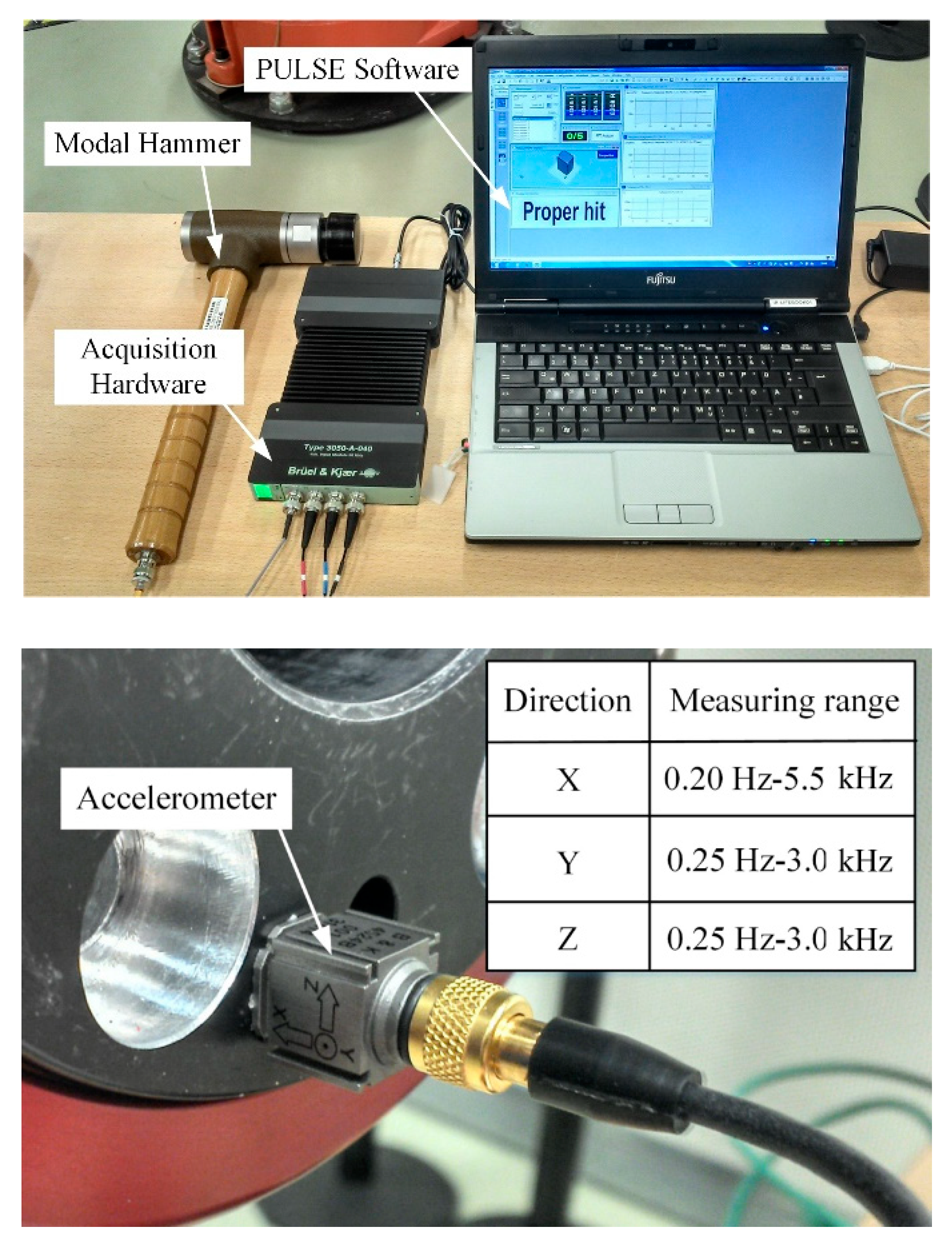
2.1. Configuration of the Experimental Modal Test

This analysis applies the modal analysis system, which is produced by the Bruel & Kjaer (B&K) company. The system contains four parts: a modal hammer, an accelerometer, acquisition hardware, and PULSE software (Figure 1).

The modal hammer is used to exert an impact to excite the structure. An 8208 hammer is used in the experiment, which is designed for excitation on a medium to a very large structure. It has a mass of 1.36 kg, and the maximum measuring range can reach up to 22,200 N. Four types of impact tips are offered: a hard tip, a tough tip, a medium tip and a soft tip. The accelerometer is attached onto the end effector of the robot, which is a three-directional B&K 4524 transducer (

Table 1. Specifications of the accelerometer and the modal hammer [20,21].

Device	Type	Dynamic Characteristics	Unites	Value
Accelerometer	B&K 4524 transducer	Measuring Range	m/s2	±500
		Amplitude Response ±10%	Hz	X: 0.2 to 5500 Y: 0.25 to 3000 Z: 0.25 to 3000
		Residual Noise (1 to 6000 Hz) Broadband	mg	X: <0.4 Y: <0.2 Z: <0.2
		Transverse Sensitivity	%	<5
Modal hammer	B&K impact hammer 8208	Sensitivity	mV/N	0.225
		Full Scale Force Range Compression	kN	22.2
		Linear Error at Full Scale	%	<±2

). The transducer and modal hammer are connected to the four input channels of the acquisition hardware, which is a type 3050-A-040 from B&K [18]. The data are then transmitted by this acquisition hardware to the computer for vibration analysis with PULSE software (Type 7770) [19].

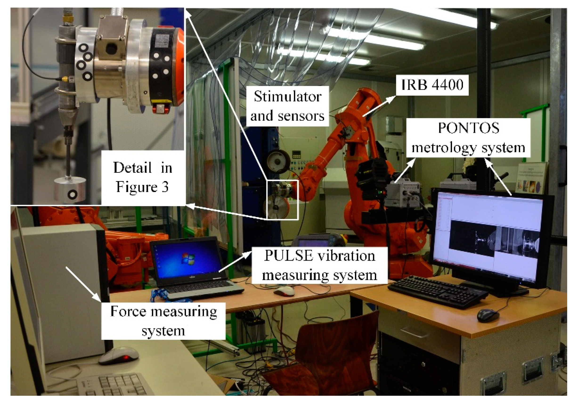
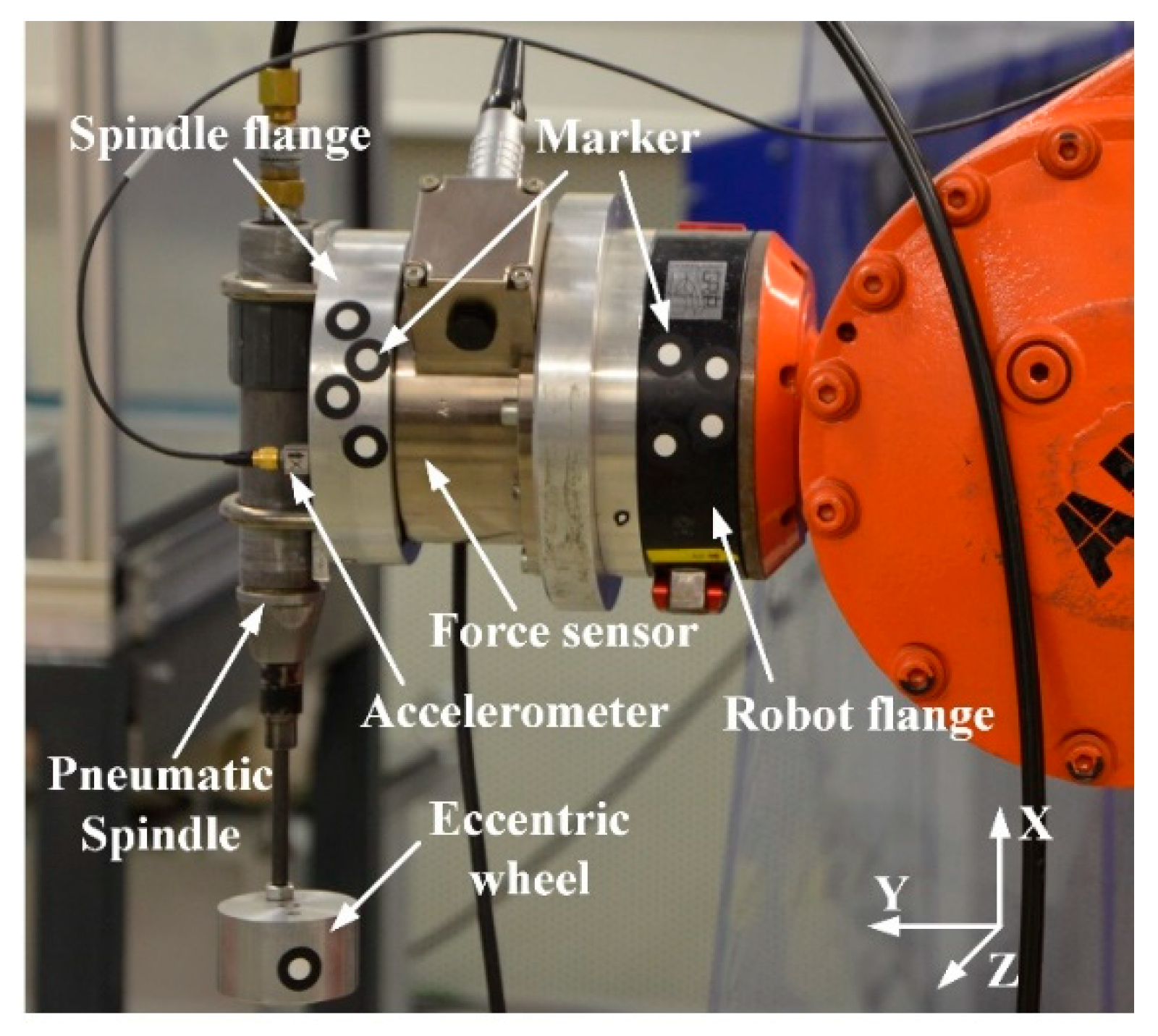
2.2. Configuration of the Experimental Modal Test

The configurations of the forced vibration experiment setup are illustrated in Figure 2 and Figure 3. The setup contains six components: the IRB 4400 industrial robot, the PONTOS metrology system, the PULSE vibration measuring system, the stimulator, the force sensor and the accelerometer.

The IRB 4400 robot is designed for robotic machining. The main applications are cutting, deburring, grinding and polishing. The maximum reach of its arm is 1.96 m, and the payload can reach up to 60 kg. Its position repeatability can reach 0.19 mm.

The high-speed camera measuring system used in this work, named PONTOS, is developed by the Gesellschaft fuer optische Messtechnik (GOM). The maximum camera resolution can reach 2048$\times$2048, and the corresponding frame rate can reach 1080 Hz. Based on the triangulation principle, its accuracy can reach 0.001 mm depending on the measuring area. The static position is measured with this metrology system for 7 s to obtain the actual accuracy. The results show that the absolute position accuracy values of the measuring system are X = 0.0016 mm, Y = 0.0019 mm and Z = 0.0051 mm [22]. The Z direction has the lowest accuracy because it is in the direction of the focal depth axis. The metrology system tracks the robot’s motion by identifying a special marker. As shown in Figure 3, markers are attached on the robot flange to track its motion. A measuring frequency (frame rate) of 500 Hz is set to track the vibration displacements. Specified parameters are stated in the table below (

Table 2. Parameter settings in the PONTOS system.

PONTOS System	Value
Focal length of lens	35 mm
Measuring volume	400 × 400 mm
Frame rate	500 Hz
Resolution	1024 × 1024 pixels

).

To measure the vibration, a stimulator and variant sensors are installed on the robot. From right to left in Figure 3, the force sensor is installed on the flange of the robot’s sixth axis. The stimulator is mounted on the force sensor, while the accelerometer is fixed on the spindle flange. These objects installed on the robot flange have a total weight of 4.7 kg. The stimulator consists of two components: a pneumatic spindle and an eccentric wheel (Figure 3). By regulating the air pressure, different vibration frequencies can be obtained. The type of pneumatic spindle is SRD 645, which is produced by BIAX Company (Greenville, WI, USA). Under a pressure of 8 bar, the spindle can reach 45,000 rpm. To provide a certain excitation force under different rotating speeds, two methods are used to achieve this requirement. One method changes the eccentric distance. The other method changes the weight of the eccentric wheel. As a result, two eccentric wheels of different weights are designed with two different eccentric distances.

PULSE vibration measuring system

In the experimental modal analysis, PULSE software is used to analyze the FRF with the data from the accelerometer and impact hammer. In this experiment, the software is used to monitor the instant vibration frequency, and obtain the required excitation frequency through regulating the pneumatic spindle. As shown in Figure 4, the PULSE software displays the data in three groups. The right graph shows the instant vibration signal from the accelerometer, which displays the signal in an instant period of one second. The upper left graph shows the fast Fourier transform of the vibration signal in one second. The lower left graph shows the 3D display of the amplitude of the vibration signal in the time and frequency domains. The x-axis is the frequency domain set from 0 to 200 Hz. The y-axis is the total measuring time, and the color contour provides the vibration amplitude. The domain vibration frequency is generated from the stimulator. It is therefore used to monitor the rotating frequency of the pneumatic spindle.

Force measuring system

This system includes one six-degrees-of-freedom force sensor (Figure 3) and a data acquisition system. The parameters of the force sensor are stated in

Table 3. Force sensor parameters.

Type	Sensing Ranges		Measurement Uncertainty
ATI Delta IP 65	Fx, Fy	Fz	Fx, Fy	Fz
	660 N	1980 N	±0.66 N	±1.98 N

. In this vibration measuring experiment, only the forces of three directions are measured with the ATI data acquisition (DAQ) system [23], which uses the DAQ F/T interface for data collection from the force sensor. The maximum data rate of this data acquisition system can reach 41.67 kHz [24]. The data sampling rate in the force measurement is set to 500 Hz.

3. Experimental Procedure and Data Analysis

This chapter is divided into three parts: Section 3.1, the first part, discusses the principle used to obtain the dynamic stiffness with modal test data and introduces the corresponding equation. Meanwhile, the excitation frequencies are planned for the direct approach based on the modal test data. Section 3.2, the second part, presents the procedure of the forced vibration measurement and the data processing and introduces the equation used for dynamic stiffness calculation; the third part, Section 3.3, compares the dynamic stiffness of the two approaches.

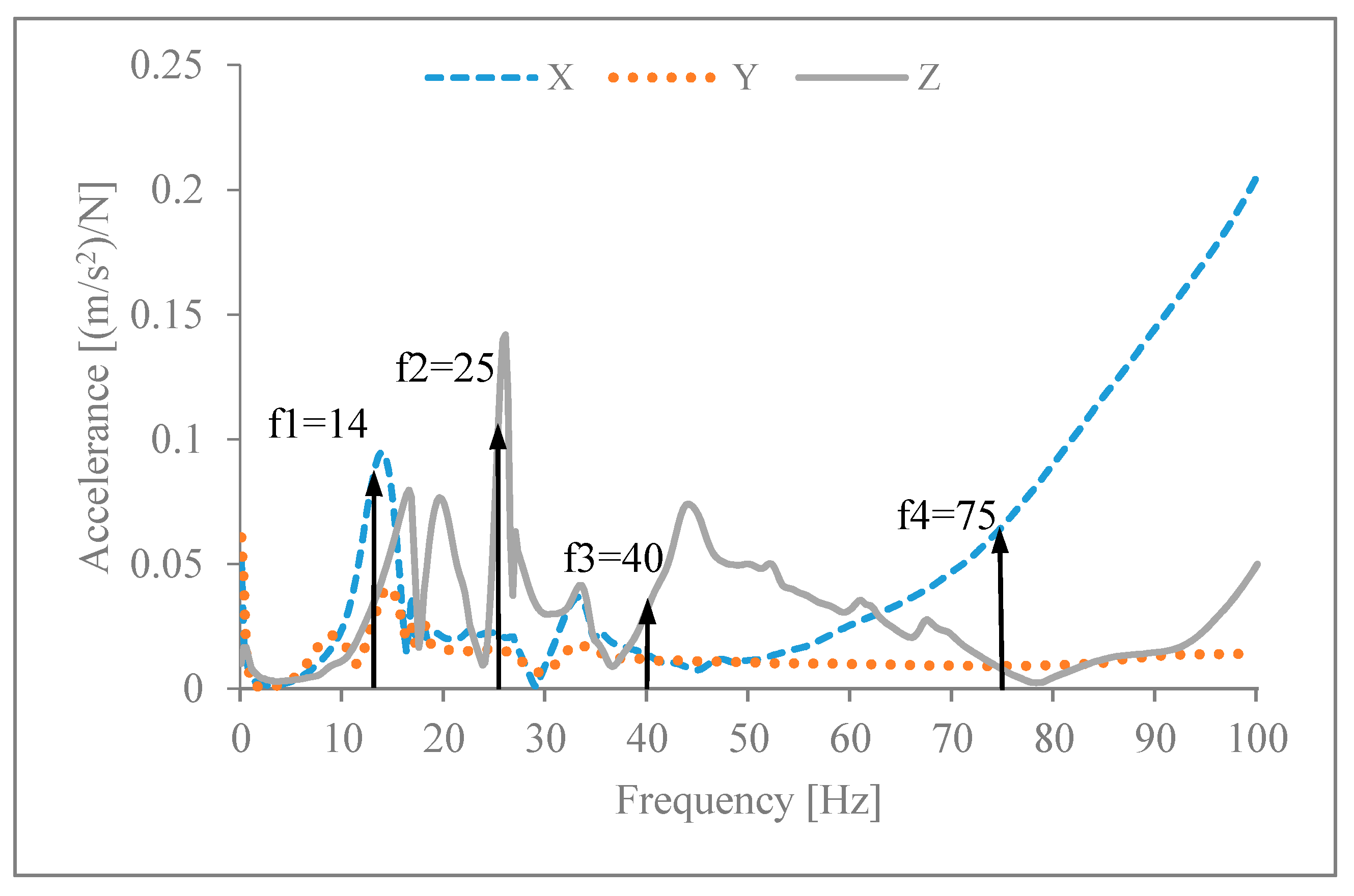
3.1. Dynamic Stiffness Calculation with Modal Test Data

A frequency response function is defined as the ratio of output to input. Three alternative estimators for the frequency response function, H1, H2 and H3, are available using a dual-channel analyzer [25]. The selection of these three estimators depends on whether there is noise in the input or output. Because impact excitation is adopted in the modal test, the noise in the input signal is negligible. As a result, H1 is used for estimating the frequency response function [26]. The equation is described below.

$$H1=\frac{G_{AB}\left(f\right)}{G_{AA}\left(f\right)}$$

(4)

where $G_{AA}(f$) is the auto spectrum and $G_{AB}\left(f\right)$ is the cross spectrum. Here, using PULSE software, H1 can be directly obtained. The dynamic stiffness $K_m$ is calculated by dividing $f^2$ by the magnitude of $H1\left(f\right)$ [27]. Here, $f$ is the frequency value.

$$K_m =\frac{f^2}{\left|H1\left(f\right)\right|}$$

(5)

An arbitrary robot position configuration in the workspace (Figure 2) is selected for this test. First, the experimental modal test is performed on the end effector of the robot to obtain the accelerance FRF of the robot. The accelerometer is fixed on the plane of the end effector (Figure 1. The characteristics of the robot are different according to the three directions (Figure 3). Hence, the FRF of each direction is measured separately when the impact force is executed in the same direction. Five impact times are planned for each direction to get the average accelerance FRF. To reduce the influence of the impact force and impact direction on the experimental results, the FRF is only recorded for analysis when the minimum coherence value is larger than 0.95. Tests with different parameters are made to ensure the appropriate setting of the modal analysis system. The details of the parameter settings are stated in

Table 4. Parameter settings in the modal analysis system.

Setting	Values
Hammer impact tip	Hard
Impact force	200–300 N
Frequency span	100 Hz
Frequency resolution	0.125 Hz
Measuring time	8 s
Average times	5

. The average times in the table concern the times of impact on the end effector. All the measurements are made in a static state without activating the motor.

The impact modal tests are carried out based on the settings above. Figure 5 illustrates the FRF H1 in three directions. This shows that the profile of H1 in each direction has its own characteristics. The peaks of the curves, which represent the eigenfrequencies of the robot in each direction, are located at different frequency values. To compare the dynamic stiffness under different frequencies, four frequency values are chosen from low to high. The frequency of f1 = 14 Hz is close to the eigenfrequency of the X and Y directions. The frequency of f2 = 25 Hz is close to the eigenfrequency of the Z direction. The other two frequencies of f3 = 40 Hz and f4 = 75 Hz are away from the eigenfrequency.

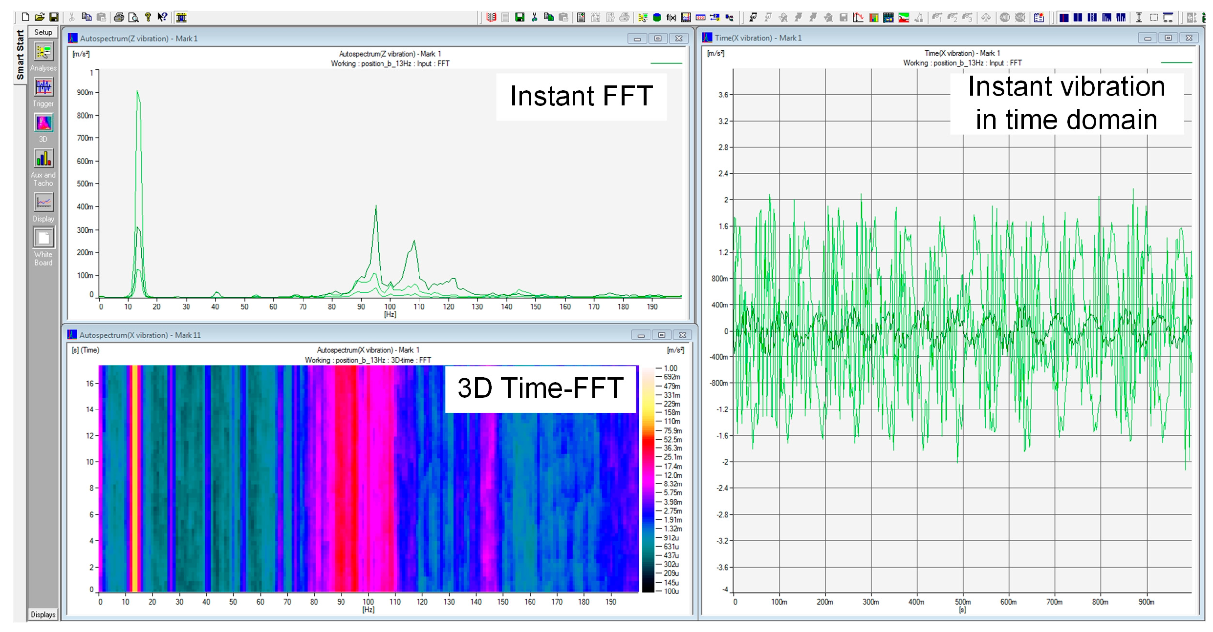
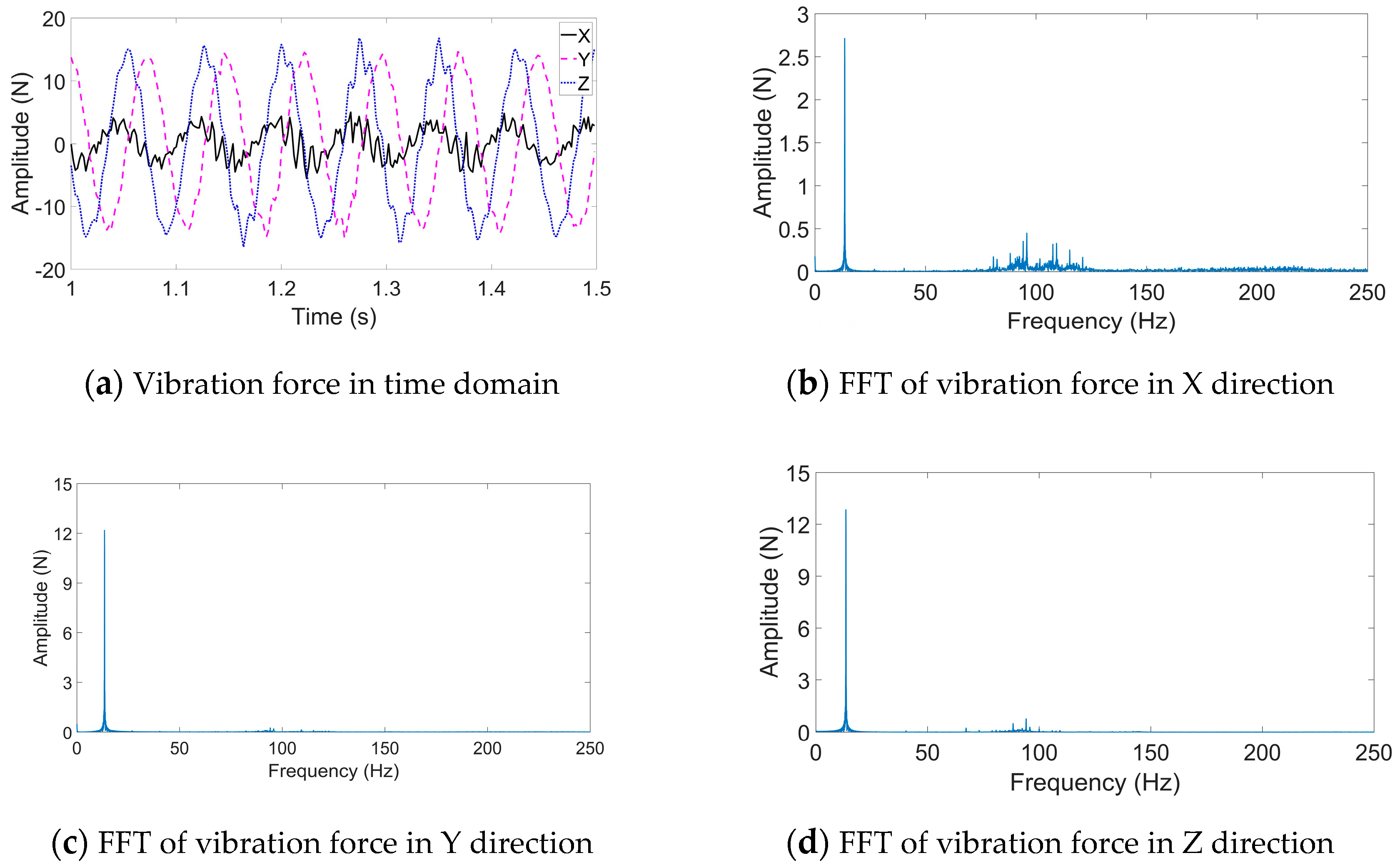
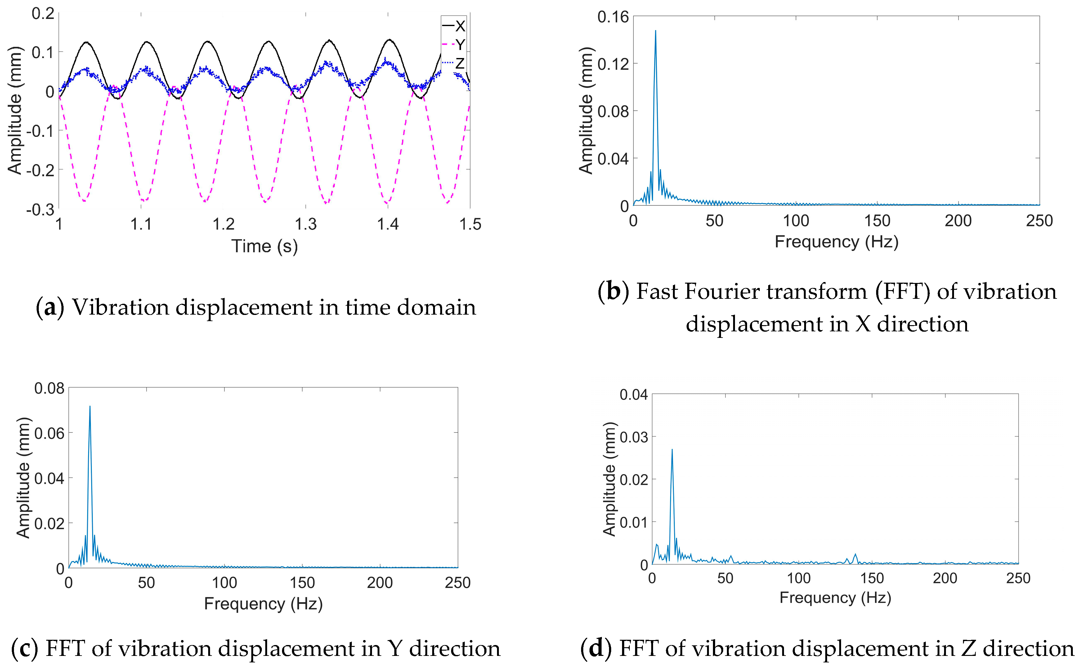
3.2. Dynamic Stiffness Calculation with Forced Vibration Data

According to the four planned excitation frequencies, the spindle is regulated to each excitation frequency. The vibration data under the condition of a 14 Hz excitation frequency are taken as an illustration of the data processing. The distribution of the forces and displacements are illustrated in both the time domain and frequency domain (Figure 6 and Figure 7). According to the force distributions in the time domain (Figure 6a), the three directions have different force amplitudes. The X direction has the lowest amplitude. This is mainly because the X direction is in the axial direction of the spindle. However, the vibration displacement has the highest amplitude among the three directions (Figure 7a). This is in accordance with the experimental results of the impact modal test, which shows the highest magnitude in the X direction at a frequency of 14 Hz (Figure 5). As the pneumatic spindle does not rotate as stably as the electrospindle, high-frequency noise can appear in the excitation vibration. Through fast Fourier transform (FFT), the vibration distribution in the frequency domain shows a high-frequency vibration at approximately 100 Hz (Figure 6b). However, the values can be ignored compared to the dominant vibration amplitude. As the spindle is manually controlled, it is difficult to set the same excitation frequency as the planned value. FFT shows that the excitation frequency is located at a frequency of 13.43 Hz. For this reason, the calculation uses the practical excitation frequency obtained from the FFT of the vibration data. Compared to the force data, the vibration displacements have much less noise. As shown in Figure 7a, noises appearing in the Z direction, which is in the direction of the focal depth axis, mainly come from the measuring system itself. Because of noise in the vibration, the peak value of the dominant excitation frequency is used to calculate the dynamic stiffness $K_e$ (Equation (6)). $F_e$ in the equation is the excitation force, and $D_e$ is the amplitude of vibration displacement.

$$K_e =\frac{F_e}{D_e}$$

(6)

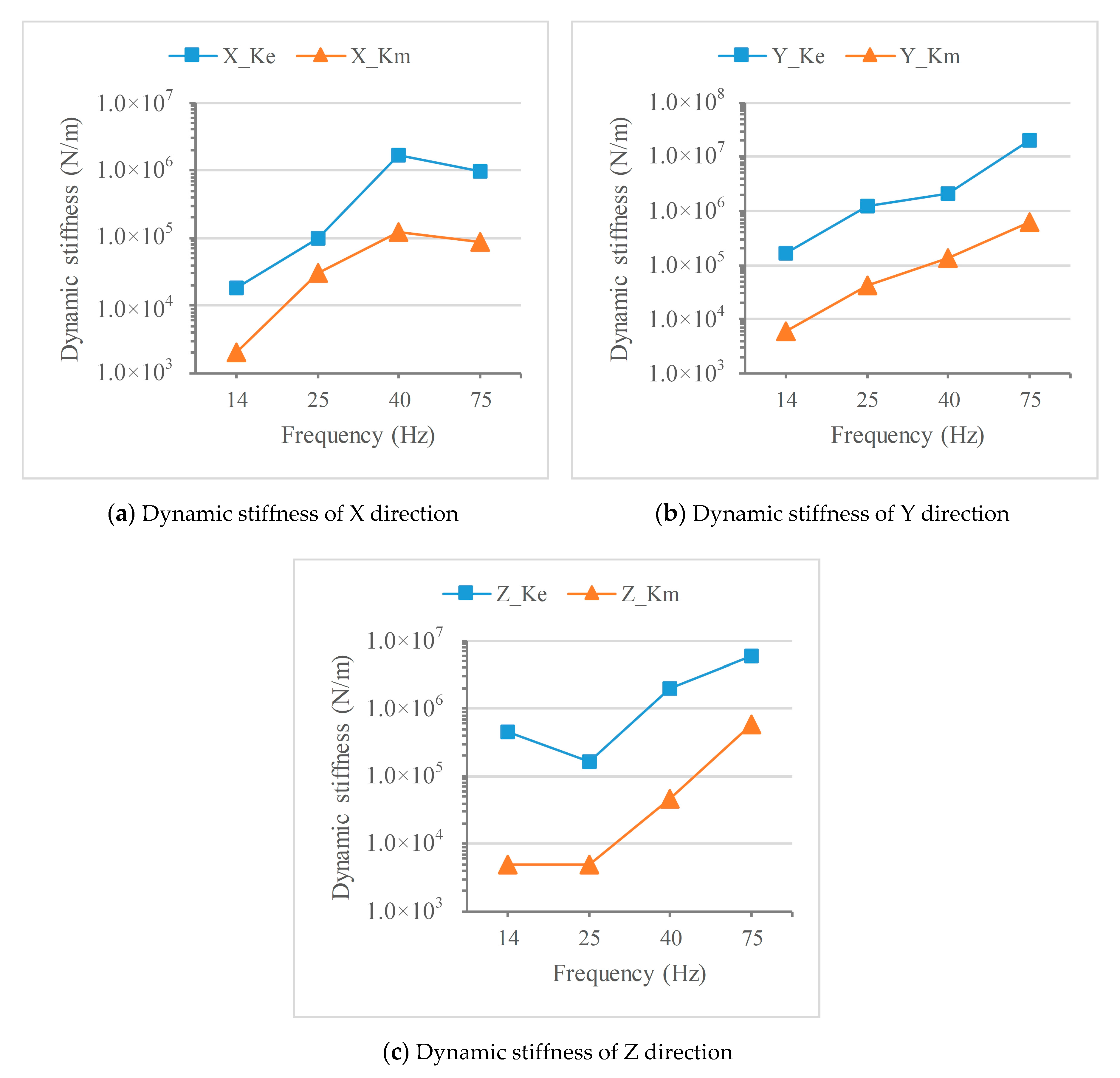
3.3. Dynamic Stiffness Analysis

Based on the abovementioned approaches, all data are processed to obtain the dynamic stiffness (Table 4). The distributions of the dynamic stiffness are illustrated in Figure 8. Because the values of the dynamic stiffness vary significantly, a logarithmic coordinate is used for the illustration, which shows that all values obtained by the direct approach are higher than the values of the indirect approach. The direct approach gives constant excitation on the industrial robot, and each robot joint is activated to vibrate. Compared with the indirect approach, the viscous damping of the robot joint has a greater impact on the attenuation of vibration. Therefore, the direct approach can obtain relatively higher dynamic stiffness. The distributions show a similar trend of change in each direction. However, the two distributions have their own change ratios. As shown in Figure 8c, $K_e$ has an obvious decrease from 14 Hz to 25 Hz. However, $K_m$ has a slight decrease. Both excitation frequencies are close to the eigenfrequency of the robot in the Z direction, which means that the dynamic stiffness is more sensitive to the forces and excitation frequency. As the distribution under different conditions is rather random, there is no regularity in the relationship between $K_m$ and $K_e$. The ratio of $K_e$ to $K_m$ ranges from 3.2 to 90.8. The large difference between the two types of dynamic stiffness is possible because the excitation energy implemented on the robot is totally different. In addition, there are excitation frequencies close to the eigenfrequency of the robot. The dynamic stiffness in this situation is prone to being influenced by the external excitation conditions, which contain the excitation force, robot pose, damping ratio and measurement uncertainty of the measuring equipment. Nevertheless, more experiments that have the same excitation force under different excitation frequencies should be planned to confirm whether this results in constant variance.

Regarding the values of the dynamic stiffness, different directions have their own characteristics under different excitation frequencies. For practical robotic machining, the dynamic stiffness of the direct approach is more meaningful for machining quality control. This apparently shows that the robot has a very low dynamic stiffness under excitation frequencies of 14 Hz and 25 Hz, while these two frequencies are close to the eigenfrequencies of the robot. In the external range of the eigenfrequency, both 40 Hz and 75 Hz have higher dynamic stiffness.

The dynamic stiffness at 40 Hz has slight variance in three directions. Its X direction has the lowest value of 1.678 × 10⁶ N/m, which is comparable to the static stiffness of industrial robots, whose values usually range between 10⁵–10⁶ N/m [28,29]. However, the values from the indirect approach show a large difference between the Y and Z directions (

Table 5. Dynamic stiffness of the industrial robot in each direction (10⁶ N/m).

Frequency (Hz)	$\mathbf{X}\_{\mathit{K}}_{\mathit{e}}$	$\mathbf{Y}\_{\mathit{K}}_{\mathit{e}}$	$\mathbf{Z}\_{\mathit{K}}_{\mathit{e}}$	$\mathbf{X}\_{\mathit{K}}_{\mathit{m}}$	$\mathbf{Y}\_{\mathit{K}}_{\mathit{m}}$	$\mathbf{Z}\_{\mathit{K}}_{\mathit{m}}$
14.0	0.018	0.170	0.454	0.002	0.006	0.005
25.0	0.100	1.235	0.162	0.031	0.042	0.005
40.0	1.678	2.042	1.953	0.123	0.137	0.046
75.0	0.982	19.790	6.054	0.087	0.606	0.593

). This indicates that the direct approach and indirect approach have no coherence to reflect the distribution of dynamic stiffness in each direction under the same excitation frequency. The rotation of the pneumatic spindle simultaneously brings excitation forces in two directions. This coupling effects affect the dynamic stiffness value. Therefore, the indirect approach is closer to the reality for this variance analysis.

When the excitation frequency increases to 75 Hz, the dynamic stiffness has obvious increments in the Y and Z directions, which can effectively reduce the vibration displacements in these two directions. However, the dynamic stiffness in the X direction decreases to 0.982 × 10⁶ N/m. Therefore, the robot pose configuration for the machining task should be planned by considering the direction with higher dynamic stiffness.

4. Conclusions

The dynamic stiffness of a robot in an arbitrary position has been calculated by two approaches. The results of both approaches indicate that the dynamic stiffness varies significantly in different directions. The values obtained by the indirect approach are much lower than those taken from the direct approach, which could be due to the different excitation energies and the nonlinear character of the damping ratio in the robot’s structure. As the direct approach implements more excitation energy into the robot, each joint has larger vibration amplitude than that of the indirect approach. Consequently, the viscous damping of the robot joint has much more influences on the attenuation of vibration, which leads to higher dynamic stiffness. The distribution of the dynamic stiffness of both types shows a similar change under different excitation frequencies. However, the amplitude of variation among the dynamic stiffness of the XYZ directions under the same excitation frequency is not coherent in the two types of measuring approaches. The indirect approach can be applied to compare the variance of the dynamic stiffness under different excitation frequencies, which is useful for robot pose configuration planning in machining tasks. As the direct approach implies a direct measurement of the dynamic stiffness, its value is closer to the true dynamic stiffness of the robot. However, the coupling effect of vibration generated by excitation in two directions should be considered in the experiment design. It is possible to use the value of the direct approach for optimizing the machining parameters. Considering the workload of the direct approach, the indirect approach is more practical for providing a general evaluation of the dynamic stiffness distribution of the robot under different conditions. The results show that the dynamic stiffness is related to the excitation frequency and direction. An appropriate frequency for the spindle rotating speed should be selected for robotic machining. In addition, the machining direction can be regulated according to the dynamic stiffness in each direction. When a higher surface quality is required, a direct approach can be adopted to obtain accurate dynamic stiffness for robot path planning and pose configuration. Further research will be focused on dynamic stiffness modeling for the robotic machining process.

References

1. Celikag, H.; Sims, N.D.; Ozturk, E. Cartesian Stiffness Optimization for Serial Arm Robots. Procedia CIRP 2018, 77, 566–569. [Google Scholar] [CrossRef]
2. Abele, E.; Weigold, M.; Rothenbücher, S. Modeling and Identification of an Industrial Robot for Machining Applications. CIRP Ann. Manuf. Technol. 2007, 56, 387–390. [Google Scholar] [CrossRef]
3. Pan, Z.; Zhang, H. Improving robotic machining accuracy by real-time compensation. In Proceedings of the 2009 ICCAS-SICE, Fukuoka, Japan, 18–21 August 2009; pp. 4289–4294. [Google Scholar]
4. Schneider, U.; Momeni-K, M.; Ansaloni, M.; Verl, A. Stiffness modeling of industrial robots for deformation compensation in machining. In Proceedings of the 2014 IEEE/RSJ International Conference on Intelligent Robots and Systems, Chicago, IL, USA, 14–18 September 2014; pp. 4464–4469. [Google Scholar]
5. Abele, E.; Bauer, J.; Rothenbücher, S.; Stelzer, M.; Stryk, O. Von Prediction of the Tool Displacement by Coupled Models of the Compliant Industrial Robot and the Milling Process. In Proceedings of the International Conference on Process Machine Interactions, Hannover, Germany, 3–4 September 2008; pp. 223–230. [Google Scholar]
6. Claudiu, B.; Mehdi, C.; Alain, G.; Jean-Yves, K. Dynamic behavior analysis for a six axis industrial machining robot. Adv. Mater. Res. 2012, 423, 65–76. [Google Scholar]
7. K’Nevez, J.-Y.; Cherif, M.; Zapciu, M.; Gérard, A. Experimental Characterization of Robot Arm Rigidity in Order to Be Used in Machining Operation. In Proceedings of the 19th International Conference on Manufacturing System-ICMaS, Bucarest, Romania, 11–12 November 2010; Volume 5, pp. 153–156. [Google Scholar]
8. Huckaby, J.; Christensen, H.I. Dynamic Characterization of KUKA Light-Weight Robot Manipulators; Georgia Institute of Technology: Atlanta, GA, USA, 2012. [Google Scholar]
9. Abele, E.; Fiedler, U. Creating Stability Lobe Diagrams during Milling. CIRP Ann. 2004, 53, 309–312. [Google Scholar] [CrossRef]
10. Matsubara, A.; Tsujimoto, S.; Kono, D. Evaluation of dynamic stiffness of machine tool spindle by non-contact excitation tests. CIRP Ann. Manuf. Technol. 2015, 64, 365–368. [Google Scholar] [CrossRef]
11. Cvitanic, T.; Nguyen, V.; Melkote, S.N.; Program, P.D.; Nw, N.A.; States, U. Pose optimization in robotic machining using static and dynamic stiffness models. Robot. Comput. Integr. Manuf. 2020, 66, 101992. [Google Scholar] [CrossRef]
12. Kim, S.-G.; Jang, S.-H.; Hwang, H.-Y.; Choi, Y.-H.; Ha, J.-S. Analysis of Dynamic Characteristics and Evaluation of Dynamic Stiffness of a 5-Axis Multi-tasking Machine Tool by using F.E.M and Exciter Test. In Proceedings of the 2008 International Conference on Smart Manufacturing Application, Gyeonggi-do, Korea, 9–11 April 2008; pp. 565–569. [Google Scholar]
13. Karim, A.; Hitzer, J.; Lechler, A.; Verl, A. Analysis of the dynamic behavior of a six-axis industrial robot within the entire workspace in respect of machining tasks. In Proceedings of the 2017 IEEE International Conference on Advanced Intelligent Mechatronics (AIM), Munich, Germany, 3–7 July 2017; pp. 670–675. [Google Scholar] [CrossRef]
14. Nguyen, V.; Cvitanic, T.; Melkote, S. Data-Driven Modeling of the Modal Properties of a Six-Degrees-of-Freedom Industrial Robot and Its Application to Robotic Milling. J. Manuf. Sci. Eng. 2019, 141, 1–12. [Google Scholar] [CrossRef]
15. Bauchau, O.A. Flexible Multibody Dynamics; Solid Mechanics and Its Applications; Springer: Dordrecht, The Netherlands, 2011; Volume 176, ISBN 978-94-007-0334-6. [Google Scholar]
16. Zimmermann, S.A.; Berninger, T.F.C.; Derkx, J.; Rixen, D.J. Dynamic modeling of robotic manipulators for accuracy evaluation. In Proceedings of the 2020 IEEE International Conference on Robotics and Automation (ICRA), Paris, France, 31 May–31 August 2020; pp. 8144–8150. [Google Scholar]
17. Abele, E.; Bauer, J.; Hemker, T.; Laurischkat, R.; Meier, H.; Reese, S.; von Stryk, O. Comparison and validation of implementations of a flexible joint multibody dynamics system model for an industrial robot. CIRP J. Manuf. Sci. Technol. 2011, 4, 38–43. [Google Scholar] [CrossRef]
18. Bruel & Kjaer. Type 3050:Multi-Purpose 4- and 6-Channel Input Modules. Available online: https://www.bksv.com/en/products/daq-data-acquisition/lan-xi-data-acquisition-system/daq-modules/type-3050 (accessed on 12 November 2020).
19. Bruel & Kjaer. System Data:Software for PULSE LabShop. Available online: https://www.bksv.com/-/media/literature/Product-Data/bu0229.ashx (accessed on 12 November 2020).
20. Bruel & Kjaer. Cubic Triaxial CCLD Accelerometer Types 4524, 4524-B and 4524-B-001. Available online: https://www.bksv.com/media/doc/Bp2076.pdf (accessed on 12 November 2020).
21. Brüel&Kjaer. Heavy-Duty Impact Hammers: Types 8207, 8208 and 8210. Available online: https://www.bksv.com/-/media/literature/Product-Data/bp2079.ashx (accessed on 12 November 2020).
22. Wu, K.; Brueninghaus, J.; Johnen, B.; Kuhlenkoetter, B. Applicability of stereo high speed camera systems for robot dynamics analysis. In Proceedings of the 2015 International Conference on Control, Automation and Robotics, Singapore, 20–22 May 2015; pp. 44–48. [Google Scholar]
23. ATI Industrial Automation. F/T Sensor: Data Acquisition (DAQ) Systems. Available online: https://www.ati-ia.com/app_content/documents/9620-05-DAQ.pdf (accessed on 12 November 2020).
24. ATI Indusrial Automation. F/T System Interfaces. Available online: https://www.ati-ia.com/products/ft/ft_SystemInterfaces.aspx (accessed on 12 November 2020).
25. Bilošová, A. Modal Testing. 2011. Available online: https://moodle2.units.it/pluginfile.php/75129/mod_resource/content/1/EMA.pdf (accessed on 8 November 2020).
26. Brandt, A.; Wiley, J. Noise and Vibration Analysis: Signal Analysis and Experimental Procedures, 1st ed.; John Wiley & Sons, Ltd.: Hoboken, NJ, USA, 2010; ISBN 978-0-470-74644-8. [Google Scholar]
27. Brüel&Kjaer. Simplified Measurement of Complex Modulus. Available online: https://www.bksv.com/media/doc/BO0218.pdf (accessed on 8 November 2020).
28. Bu, Y.; Liao, W.; Tian, W.; Zhang, J.; Zhang, L. Stiffness analysis and optimization in robotic drilling application. Precis. Eng. 2017, 49, 388–400. [Google Scholar] [CrossRef]
29. Alici, G.; Shirinzadeh, B. Enhanced stiffness modeling, identification and characterization for robot manipulators. IEEE Trans. Robot. 2005, 21, 554–564. [Google Scholar] [CrossRef] [Green Version]
Figure 1. Modal analysis system configuration.
Applsci 10 08332 g001
Figure 2. Configuration of vibration experiment setup.
Applsci 10 08332 g002
Figure 3. Stimulator and sensors.
Applsci 10 08332 g003
Figure 4. Interface of PULSE software in the vibration measurement.
Applsci 10 08332 g004
Figure 5. Accelerance frequency response function (FRF) H1 in three directions.
Applsci 10 08332 g005
Figure 6. Vibration force in time and frequency domains under 14 Hz excitation frequency.
Applsci 10 08332 g006
Figure 7. Vibration displacement in time and frequency domain under 14 Hz excitation frequency.
Applsci 10 08332 g007
Figure 8. Dynamic stiffness distributions under two calculation approaches.
Applsci 10 08332 g008