Abstract
The present work is focused on the analysis of flood scenarios for the settlements near the Danube discharge area into the Black Sea. From this perspective, the aim of the research is the development of flood extension maps for localities in the Danube Delta. The emphasis is on collecting the data and information needed for the entire analysis process, such as hydrological data on Danube flows and water levels (which were analyzed for 51 years), topo-bathymetric data (where 1685 cross sections were processed, measured on an 87-km section of the Danube), a digital terrain model (DTM), and others. Two methods of flood scenario analysis for the localities targeted were used in this paper. The first method was an analysis of the flood scenarios by modeling a real scenario, where it was supposed that a 20 m breach appeared in the dam which protects the localities and remained present for 24 h. The second method consisted of a Geographic Information System (GIS) analysis (static from a hydraulic point of view), where the maximum water level was superimposed over the DTM. This corresponded to a scenario in which the breach in the flood-control levee remains present for a longer period. The validated results show that the dynamic method is more efficient than the static method, both in terms of estimated flooded surfaces and in terms of simulation accuracy (taking into account more input parameters than the static method). Thus, from the obtained simulations it was observed that applying the dynamic method resulted in smaller flooded surfaces in the settlements analyzed than when considering the static method. In some cases, the differences between the flooded surfaces reached up to about 22%. This information is important and of general interest since it can be used in various fields of work, such as flood defense strategies, and investment promotion activities in the Danube discharge area or similar locations.
1. Introduction
Although, extremely important for humanity in many respects, water also carries a significant destructive potential, causing damage to people through the occurrence of natural hazards such as floods [1]. Floods represent the most common hydrological hazard in Romania, as well as in many places all over the world [2]. Over time, floods have occurred in various regions of the country, causing particularly significant damage, both in terms of infrastructure, and in terms of households and agriculture [3].
Floods are natural phenomena that cannot be prevented. Nevertheless, some human activities (such as the increasing number of human settlements and economic assets in floodplains, as well as the reduction of natural capacities for water retention through certain land uses) together with climate change, contribute to the increased likelihood of floods and their negative impact. The study of these phenomena in the Danube Delta is important because recent flood events have increased in number and magnitude in this area, and many settlements have been affected. This river flooding triggers significant level and flow variations along the river, endangering infrastructure elements (mainly dykes of settlements), agricultural areas, and households [4].
Beltaos [5] used the Hydrologic Engineering Center’s river analysis system (HEC-RAS) to evaluate spring breakup of the ice cover which is the main agent of flooding and replenishment of the Peace–Athabasca Delta. This study showed that different ice-jam scenarios indicated that jams of moderate, rather than extreme, length were more effective in flooding the Delta. In addition, Nones [6] used numerical modeling of the hydro-morphodynamics of a distributary channel of the Po River Delta (Italy) during the Spring 2009 flood event to show how the dimensions of the river plume can influence the evolution of the prodelta, while having a rather negligible effect inland, because of the major stresses induced by the high river discharge during the flood event. Another interesting study was carried out by Win [7] who evaluated the flooding of vulnerable areas by a different return period flood, by using the Hydrologic Engineering Center’s river analysis system (HEC-RAS) model in the Ayeyarwady Delta Region, Myanmar. The results of this study showed that the arable land and forest were the most vulnerable to different return period flooding. The HEC-RAS software represents an affordable method for this type of assessment.
According to Molina [8], the acquisition, management, and use of spatial data are essential for quality of water resource studies. Thus, several geomatic methods serve hydrological modeling, and emphasizing the generation of cartographic products. Furthermore, a study developed by Zazo [9] on the analysis of flood modeling through innovative geomatic methods, aimed to evaluate the flood risk, while assessing the suitability of an innovative technique. The results of this study showed that the developed methodology and technology allowed for a more accurate riverbed representation. Gergeľová [10] evaluated the selected sub-elements of spatial data quality on 3D flood event modeling. The study focused on the evaluation of the state of spatial information quality. The results of the study show that the combination of different type of the input data, like a digital relief model combined with geodetic or topographical data, can provide a redefined 3D model. This type of input data influences directly the hydrodynamic modeling process.
In the Danube Delta, floods are hydrological events that can occur at any scale. These phenomena have appeared more and more often in the last decades. Due to the geographical position, and the specifics of the area, as well as the unique natural character of the Danube Delta, hydrological hazards (heavy showers, sometimes accompanied by hail, river flooding, strong storms, extreme temperatures, etc.) frequently arise [11]. The flooding process is influenced by the rate of the Danube water level rise. Depending on their magnitude, they proportionally affect a certain part of the Delta surface, and especially the settlements along the main branches of the river [12].
The Danube Delta is a very dynamic area, whose main direction of evolution is horizontal and vertical growth. The character of the water level variations in the Danube Delta presents a series of particularities specific to the discharge area of the Danube into the Black Sea. Of course, the variation of the water levels in the Delta is, first of all, closely related to the variation of the water supply at the entry point at the Chilia Ceatal, and to the variation in the wind where the water flows into the Black Sea [13,14].
General practice has shown that floods cannot be prevented. Still, they can be managed, and their effects can be reduced through a systematic process that leads to a series of measures and actions designed to help reduce the hazards associated with these phenomena [15]. The capacity of flood reservoirs is influenced by the scale of each type of river flooding. Similar river flooding, in terms of maximum water level reached and duration, can find the inside area of the delta in different stages of initial accumulation, which contributes to emphasizing the complexity of the flooding phenomenon. Therefore, due to the varied relief and the particularities of the flow regime of each flood, the flooding process across the entire delta becomes particularly complex [16].
Floods in the Danube Delta become natural disasters when they affect human settlements. The vast majority of localities in the Danube Delta are situated in floodable areas, especially those distributed along the main branches of the Danube, presenting a high hazard of flooding [17]. The hazard is determined by the failure of the dams to defend the localities, due to severe river flooding on the Danube and its extended duration. The pressure of the flood exerted on the dyke causes it to give in, especially in vulnerable areas (a breach/rupture is created in a section of the dam), endangering homes and households [18].
For a wetland with a variety of ecosystems and biodiversity, such as the Danube Delta, one of the most important conditions is the water circulation system [19]. Different land use modifications over time of some important territories, by disregarding the effect of the floods, have caused a decrease of the storage capacity of the Delta by approximately 34%, and at the same time, modified the environmental and social characteristics [20]. This area is of great interest for flood analysis because the settlements in the Danube Delta have a long history of destructive events. A good amount of Danube water is taken by the main branches and distributed to the mouths at the Black Sea [21].
In the Danube Delta there is a danger of spillage for dammed areas in places where the dam tamping phenomena (dam falling) has occurred, and even the major danger of infiltration due to the very long duration of river flooding on the Danube [22]. At the same time, there is the permanent danger of erosion, sometimes accompanied by landslides, that endanger homes and households.
Identifying the scenarios in which river flooding can occur on the Danube is central in the broader flood scenarios analysis. Once the context of the specific flood problem to be addressed has been established, the hazard of flooding must be identified and analyzed [23]. This involves hydrological and hydraulic analyses using specialized software that models flood phenomena. [24] Some of the key elements resulting from the flood scenarios analysis are flood extension maps, as well as tables and graphs showing the state of play during the unfolding of these phenomena [25]. The first problem that arises when elaborating flood maps is the choice of hydrological situation when the water levels on the main branches are high, and this must be considered and analyzed [26].
Therefore, the main objective of this study was the evaluation of two simulation methods to assess extent of flooding for the settlements in the Danube Delta, by using low-cost equipment and less time-consuming simulation methods, to obtain flood maps corresponding with different flood scenarios. The flood extension maps depict the potentially flooded areas of the settlements, as a result of the occurrence of a breach (rupture) in the dyke. Furthermore, a comparison was made between the results obtained using two methods that analyze different scenarios of breaching the dyke. The analysis will be applied to the settlements on the course of the Sulina branch, located near the area where the Danube discharges into the Black Sea.
2. Study Area and Data
2.1. Study Area
The Danube Delta is located in the eastern extremity of Romania and covers 2.5% of the country’s area. The Danube Delta, including the peripheral lake areas, extends North to 45°27′ northern latitude (Chilia branch, 43 km), South to 44°20′ (Cape Midia), West to 28°10′ E (Cat’s Bend) and East to 29°42′ E (Sulina) [27]. The Danube Delta is a complex environment, governed by the interactions between the Danube River and the Black Sea [28].
Ecosystem services, provided by the Danube Delta, are very diverse, due to the heterogeneity and high dynamism of ecological systems in the area [29].
As a result of the decrease of the floodplains in the Danube Delta area, the nutrient retention capacity has decreased, so the Danube waters are affected by strong eutrophication. These phenomena affect trophic cycles, leading to a decrease in biological diversity through the disappearance of some species, many of which have high landscape and even economic value [30]. The Delta area requires major investment and the development of quality studies on the modeling of flood phenomena. The transformation of wetlands into terrestrial ecosystems and the modification of ecosystem structures have decreased the capacities of floodable surfaces, as well as ecological, economic, recreational, aesthetic, and educational capacities.
In the present study, the settlements located along one of the three main branches of the Danube (the Sulina branch with a length of approximately 71 km), which partly ensure the water flow to the Black Sea, were taken into account (Figure 1). The settlements analyzed were Partizani, Ilganii de Sus, Vulturu, Maliuc, Gorgova, Mila 23, and Crișanand Sulina. These localities are vulnerable to the high-water level of the Danube.
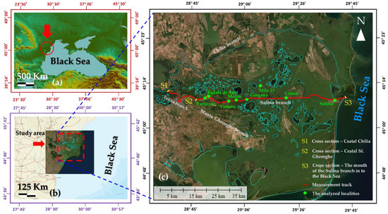
Figure 1.
Geographical locations of the settlements along the Sulina branch considered for this study, (a) the study area superimposed on the topographic map; (b) the geographical position of the settlements superimposed on the ortho-photomaps of the Danube Delta (the green dots are the settlements located along the Sulina branch) and the patch on which topo-bathymetric measurements were performed (S1, S2 describe the cross sections measured in the first part of the river, and S3 describes the cross section measured in the river’s second part); (c) the study area superimposed on the digital terrain model.
These waters, entering the delta, reach the sea following several flow paths; the Chilia branch, followed by the branches of the secondary Chilia delta and the Tulcea branch, splitting onwards into the Sulina and Sfantu Gheorghe branches. Between the main water flow routes through the Danube Delta and the interior of the delta, and between these routes and the areas outside the delta, as well as between the delta and the sea and inside the delta, there are several connecting routes for water circulation, which play a particular role in the hydrological regime of the delta [31]. Through these routes, a natural accumulation reservoir role is played by the interior of the delta and by some outer areas, and secondary routes of water flow to the sea appear. The regime of this natural reservoir is determined by the flow of the Danube at the starting point of the Delta [32].
A major flood event in the Danube Delta was identified in July 2010 and examined in the present study. Major floods were generated by the appearance of significant water flow on the Danube. The flow resulting from the river flooding was of 16,600 m3/s, as opposed to the 6658 m3/s mean flow (between 1965–2015), registered at the Tulcea-port hydrometric station. The maximum level of the flood was recorded on 6 July 2010 as 4.95 m, measured for the Black Sea Sulina system, opposed to the 2.50 m mean level. A flow hydrograph with a peak discharge of 16,600 m3/s was created and validated in the present study for the analysis of flood scenarios for settlements distributed along the Sulina branch [33].
2.2. Data
Most of the time, floods occur as a result of high-water levels that are characterized by reaching a maximum point in terms of flow value. Thus, the available hydrological data for 51 years, between 1965 and 2015, were studied.
Thus, Figure 2 presents the variation of the average annual flows at the Danube Delta entrance point, distributed by years, throughout the analysis period.
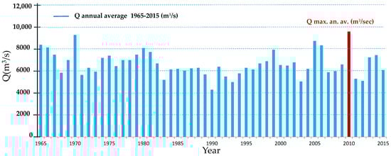
Figure 2.
Variation of the average annual flows at the entrance to the Danube Delta, between 1965 and 2015.
The average flows of the Danube were then calculated at intervals of 5, 6, and 10 years, respectively, both at the delta entry point and on the three main branches (1965–1970, 1971–1980, 1981–1990, 1991–2000, 2001–2010, 2011–2015) (Table 1).

Table 1.
Average flows of the Danube at intervals of 5, 6, and 10 years, respectively, at the entrance to the Delta and on the three main branches (between 1965–2015).
From the analysis of this data, it could be concluded that the most probable value of the average flow over the entire analysis period at the entry point into the delta is between the approximate limits of 6700–6750 m3/s. The data analysis also shows that the maximum annual peak flow was recorded in 2010, a value of 16,600 m3/s, followed by 1970. This can be explained by taking into account variations in average annual flows over time.
The flow that entered from the branches of the Danube into the main units of the delta in the period 1965–2015 was reduced. This reduction was caused by the alluvial clogging of some canal sleepers and the closure of others that generated clogging in the adjacent spaces [34]. From the longer data series, starting with 1996, it was found that the years in which average annual flows of less than 6000 m3/s were recorded were the years 2003, 2007, 2008, 2011, and 2012, and average annual flows of more than 8000 m3/s were recorded in the years 2005, 2006, and 2010. River flooding usually occurs during the high-water phase [35].
The high-water levels of the 2005, 2006, and 2010 floods were imposed by the restriction of the freedom space of the lower Danube by damming the meadow, combined with significant rainfall.
In addition, in July 2010, large-scale floods occurred in the Danube Delta as a result of a strong river flooding on the Danube. This phenomenon caused the almost complete flooding of settlements protected with local works or those simply unprotected, but also the rupture of some dams that had been dimensioned according to a class of greater importance (such as hydro-technical works). At the same time, the fact that there was an accumulation of water coming almost simultaneously from the flood in the whole delta, combined with the fact that the discharge to the sea was cumbersome, led to prolonged periods of water pressure on the protective dams.
The year 2010 represented the reference year for the present study, considering the floods that took place in the Danube Delta. Figure 3 shows the monthly situation of water levels for 2010 and 2003. Levels were recorded at the Tulcea-port hydrometric station, located upstream of the studied area. The data analysis for 2003 and 2010 was based on a series of daily data (daily recordings) of the Danube water levels. From the analysis of the data presented in Figure 2 and Figure 3, it was found that in 2010, the water level of the Danube reached the maximum value of 4.95 m (regarding the Black Sea at Sulina).
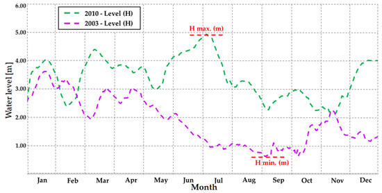
Figure 3.
Monthly evolution of the Danube water levels at the Tulcea-port hydrometric station during 2003 and 2010.
In 2003, the historical minimum water level of the last 20 years was registered in September, due to the warm period of the year and low rainfall. This minimum generally appears most frequently in October, but also in the first and second half of September. The historical minimum water level reached the value of 0.61 m (with reference to the Black Sea at Sulina) and represented a dry year for the Danube Delta. Figure A1 (Appendix A) shows the monthly distribution of the minimum and maximum water levels at the Tulcea-port hydrometric station in 2003 and 2010.
The water flow registered on the Danube in the summer of 2010, corresponding to the maximum level of 4.95 m with reference to the Black Sea Sulina, reached a peak of approximately 16,600 m3/s, at the Tulcea-port hydrometric station.
3. Materials and Methods
The present study comprises the analysis of two scenarios where ruptures occur in the settlements’ dykes in conditions of maximum levels on the Danube. The difference between these two scenarios is how long the breach remains open in the dyke. Thus, the first scenario of flood analysis was applied to the settlements by modeling a real scenario with the occurrence of a 20 m opening (breach) in the dyke, remaining present for 24 h at the maximum water levels of the Danube. The second scenario of flood analysis was applied to the settlements through a Geographic Information Systems (GIS) analysis (static from a hydraulic point of view), consisting of superimposing the information corresponding to the maximum water level over the digital terrain model. It corresponds to the most unfavorable scenario, namely the breach/breaches remaining present in the dyke at the same time as the maximum water levels of the Danube for a longer period (more than one day).
For the analysis of the dam breaching scenarios, two methods were used: the dynamic method for the first scenario, and the static method for the second scenario. The steps followed are summarized in a process diagram (Figure 4).
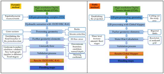
Figure 4.
Diagram indicating the methodology considered in the present work, and which describes the main steps.
According to the figure above, the diagram of the applied process involves a continuous, interactive, and dynamic process. These stages do not form a linear process but move sequentially from one step to another and vary depending on the results of each stage. It is clear from the scheme that the input data are very important in flood scenario analysis.
The data collection process begins with a regional assessment, an exploratory phase, or even an investigation, which provide input for the proposed diagram [36]. Following the data collection, in the first phase the raw data are obtained (in this case, the hydrological data, water flows and water levels, and topo-bathymetric data, transverse profiles, topographic maps, the digital terrain model, ortho photomaps, satellite images, etc.), representing the primary data that require elementary processing for further use [37]. The data are obtained from external sources, such as administrative flow data, existing studies and research, maps, photographs, or internal sources (collected during the study using an appropriate methodology). The accuracy of the results of the analysis depends on the accuracy of the raw data [38].
As shown in Figure 4, the proposed methodology combines two methods of analysis. In the approach of each method, we need input data, such as the digital terrain model, hydrological data, topo-bathymetric data, and topo-geographic data for the Danube Delta area.
The basic element that the two methods are applied to is the digital terrain model (DTM). The DTM has the role of rendering the terrain configuration continuously from a spatial point of view, and can be manipulated by computer programs. Today, light detection and ranging (LIDAR) technology is known as an important source of geospatial information. The benefits of this technology are particularly valuable in a wide range of scientific and professional fields, such as land monitoring, hydraulic modeling of rivers/streams, and more [39,40]. The data from the DTM used in this study (Figure A2) shows the terrain with a high degree of accuracy, for both axis direction: horizontally, 0.5 m × 0.5 m, and vertically, 0.05 m. The accuracy is more important than resolution in hydraulic and hydrological modeling research and GIS analysis. The data files contain spatial terrain height data in a digital format, usually in a rectangular grid.
As the study area considered overlaps with an extremely large space, the DTM had to cover the entire area of the Danube Delta itself, in order to have good data processing for the hydraulic modeling and the GIS processing. The content of the digital model of the land supports the design of the flood protection lines for the settlements, and at the same time creating a useful tool for analyzing the dynamics of hydro–geo–morphological phenomena, which are very dynamic in the study area. The correlation between these phenomena and land use can only be made on such a model. The hydro–geo–morphological units were mapped using a LIDAR based DTM [41].
This DTM was obtained from LIDAR measurements performed within the project “development of a high resolution digital cartographic support necessary for the implementation of plans, strategies and management schemes in the Danube Delta Biosphere Reserve”—CARTODD [42].
The high resolution digital cartographic framework developed in this project comprises several components: the DTM, the digital elevation model (DEM), elevation classes (EC), and ortho photomaps (OFM). These components represent the foundation layer for approaching the two methods in this study. They were developed by processing primary cartographic data, obtained by modern methods (data collection by LIDAR method), and the high accuracy of ortho photomaps (2.5 MP) allowed detailed visualization of the areas of interest. The development of the numerical field model (NFM) with the LIDAR method was based on the detection of the echo/retro diffusion of a laser pulse, and the measurement of the round-trip flight time of the aircraft-scanned object (e.g., a land surface). The flight parameters were chosen to achieve the required precision objectives, in altitude on the Z axis of 5 cm, and the necessary and sufficient density of points (i.e., average 4–5 pts/m2), to correctly detect the dams, taking into account the random distribution of the point cloud. The whole process of hydraulic modeling and GIS processing in flood scenarios analysis depends on the accuracy of the digital terrain model.
The interpolation method for minor riverbeds used in this study was inverse distance weighting (IDW). This method is a deterministic spatial interpolation model, based on an assumption that the value at an unsampled point can be approximated by a weighted average of observed values within a circular search neighbourhood [43,44,45]. The DTM resolution for the minor riverbed was computed with a similar resolution as the LIDAR DTM (0.5 m × 0.5 m), but it was resampled up to 1 m, which allowed an easier input of data in the HEC-RAS and Global Mapper software. The main channel vertical accuracy was 0.10 m.
In order to obtain a complex digital terrain model, the area comprising the minor riverbed of the digital model was cut and replaced with a new model of the minor riverbed updated by topo- bathymetric measurements. For the new digital model of the minor riverbed, topo-bathymetric measurements were performed in the study area (along the entire length of the Sulina branch, from Ceatal Sfantu Gheorghe to the mouth at the Black Sea) and downstream of the Sulina branch (along the entire length of the Tulcea branch, from Ceatal Chilia to Ceatal Sfantu Gheorghe), resulting in 2 measured sections. These data were collected with the help of state-of-the-art equipment provided by the Danube Delta National Institute for Research and Development.
The equipment used to perform the topo-bathymetric measurements was a SonTek ADCP RiverSurveyor M9 (SONTEK Company, San Diego, CA, USA) which used 3 × 3 transducers, each with a different orientation.
The topo-bathymetric measurements were performed between the 16 and 27 of March 2020, in conditions of low water levels of the Danube river, recorded at the Tulcea-port hydrometric station, namely 0.52–0.67 m. The two calibration sections in which the hydrological measurements were performed are presented in Figure 1c (S1–S2 first river part and S2–S3 second river part). The following technical means were used for this activity: a motor boat, to the starboard side of which was fixed, with a special fastening system, a float on which the equipment for hydrological measurements was installed, an acoustic doppler current profiler (ADCP), equipped with sensors for measuring the water flow characteristic parameters, and a GPS antenna.
The primary data, measured by ADCP in a cross-section through the riverbed, provided info on water depth (H), the width of the cross-section through the riverbed, measured at water surface level, water flow, and water flow velocities, measured for the entire cross section of the riverbed. Fieldwork for hydrological measurements is presented in Figure 5. Attaching the float to the starboard side of the boat was a necessary condition so that the ADCP sensors were positioned upstream of the boat’s engine. Thus, the data measured by the sensors were not influenced by various parameters related to the boat engine (vibrations, currents induced by the engine propeller, the degree of attenuation of the water flow because of the impact with the boat’s hull, etc.).
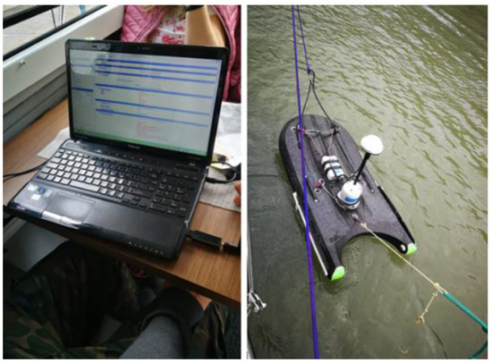
Figure 5.
Topo-bathymetric measurements with ADCP (acoustic doppler current profiler).
A GPS antenna mounting system was available at the top of the sensor unit. The antenna collects geolocation data so that data recorded by the ADCP sensors was georeferenced. The main unit of the ADCP (console) was also installed on the same floater. It picked up and connected the two signal streams (transmitted by the ADCP sensors and by the GPS antenna), and, through a radio system (transmitter-receiver), communicated wirelessly with the on-board laptop. In this laptop, the control and data collection program from the main unit (console) was running.
With this type of data collection, the bathymetric profiles were based on a large series of data (cross-sectional profiles were collected at average distances of about 50 m from each other and comprised a large number of points for each profile). The minimum distance measured between the cross-sectional profiles was 30 m (in critical regions or at river bends), and the maximum distance was 70 m (Figure A3 and Figure A4). The first measured river section was on the Tulcea branch, with a length of approximately 17 km, having as a starting point Ceatal Chilia (measured transversal profile S1), and as stopping point Ceatal Sfantu Gheorghe (measured transversal profile S2). Inside this river section, 340 transversal profiles were made from the left bank to the right bank of the river branch, cumulating between 160 and 250 points for each measured profile, depending on the width of the branch.
The second river section was measured on the Sulina branch (the analyzed settlements are distributed along this branch) on a length of approximately 70 km, having as a starting point Ceatal Sfantu Gheorghe, and as final point the mouth of the branch into the Black Sea (the interval between the measured cross-sectional profile S2, and the measured cross-sectional profile S3). Inside river part 2—1345 cross-sectional profiles were generated, with between 110 and 200 points for each measured profile (the width of the Sulina branch being variable along its entire length).
4. Results
The calibration of the hydraulic model was first performed upstream of the study area, more precisely in the Danube entrance sector in the Delta (Ceatal Chilia), and later downstream, at the mouth of the Sulina branch in the Black Sea. The calibration of the model in the HEC-RAS software was made by alternate values of the Manning roughness coefficients, between 0.025 and 0.03, and by applying the rating curve data from the Tulcea hydrometric station (Figure A5).
In the next stage (unsteady flow module), in order to define the boundary conditions, an analysis of the hydrological data of the Danube was performed, which required the description of the water flow history for a period of time.
Figure 6 and Figure 7 show two cross-sections used for model calibration, which were made on both river parts.
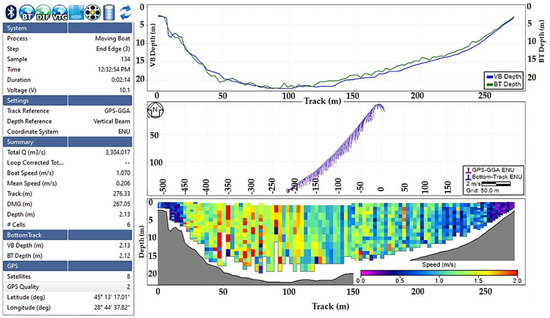
Figure 6.
Profile S1 created with the ADCP-profile trajectory, measured parameters (total flow, boat speed, average speed, measured distance, depth) and water velocity graph (velocities distributed on cells, with a colour gradient of velocity intensity, on the water column). The profile was extracted from the River Surveyor Live software used in the processing of data collected by ADCP.
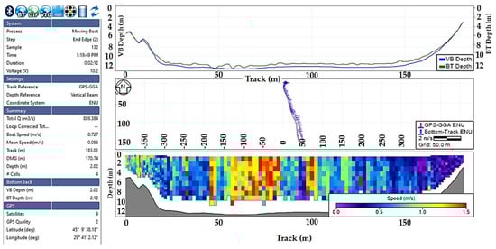
Figure 7.
Profile S3 created with the ADCP-profile trajectory, measured parameters (total flow, boat speed, average speed, measured distance, depth) and water velocity graph (velocities distributed on cells, with a colour gradient of velocity intensity, on the water column). The profile was extracted from the River Surveyor Live software (Version 4.1, SONTEK Company, San Diego, CA, USA, 2018) used in the processing of data collected by ADCP.
The absolute elevation value (Z) of the riverbed was determined by finding the difference between water surface value and a water depth value (H). The water level for the measured sections upstream and downstream of the hydrometric station was calculated using real-time kinematic positioning (RTK).
To determine the water surface level, for each cross-section of the riverbed where bathymetric measurements were performed, two methods were used to determine the elevation values. The first method consists of measurements with RTK Rover (ROMPOS) Spectra precision SP80, and the second method consists of reading the values recorded at the hydrometric stations (at Tulcea, Sulina, Sfantu-Gheorghe, Chilia-Veche, Periprava). For georeferencing the data (spatial/global referencing) we used the geographic positioning data of each point in the riverbed profile and the data on the depth of each point (absolute elevation of the riverbed, referenced to the Black Sea reference system 75-BS75). The X, Y, Z data were thus georeferenced data obtained for each point measured by ADCP in the topo-bathymetric sections on the Danube branches.
Following the GIS pre-processing of topo-bathymetric data, a new digital model of the minor riverbed was obtained. The cumulation of the two models resulted in a complex digital model with updated data on the minor riverbed. The next step was the analysis of flood scenarios using the dynamic method.
For the dynamic method, HEC-RAS 5.0.3 specialized software was used. In the next step, the complex digital terrain model was introduced into the software for defining and processing the geometric data. The geometric data used for hydrodynamic simulation were obtained using high-precision DTM, with a spatial resolution of 0.5 m × 0.5 m. The next geometric elements were the channel centerline, bank lines, the flow-path lines above the banks, and 174 cross-section cut lines, perpendicular to the direction of the river flow. It is important to note that each cross-section covered the elevations of the stream bed to the banks, with a width of about 800 m to 1500 m. These geometric features were further used in the HEC-RAS hydraulic modeling step.
An important step in hydraulic modeling is the assignment of the roughness values. The values of the Manning roughness coefficients were assigned according to the character of the riverbed, the relief, and the vegetation in the vicinity of the river. For the 2D flow area, the Manning roughness coefficient was calibrated in the range between 0.025 and 0.03. Regarding the calculation points of the 2D computational mesh, they were generated at steady intervals. The distance between the calculation points was set as a grid with a distance of 50 m on the x and y direction axes. In this way, finite elements were created for the 2D flow area.
The floodplain attributes were provided by the topography of the high-resolution DTM. Thus, through the HEC-RAS 1D/2D hydraulic model, the 2D flow area was generated in the study area and upstream, by designing polygons along the length of the river, including the analyzed settlements and by defining the boundaries. By defining these boundaries, the program was able to calculate the spread of the flood wave. The design of the polygons was made taking into account the scenario in which the dyke of the settlements is breached with an opening of 20 m maintained for one day. Figure 8 and Figure 9 show the breaches induced in the dyke of the targeted settlements. Reliable historical information is not available about the positions where dam breaching occurs. From this perspective, the locations assumed for dam breaching were established considering the most vulnerable dam zones. These vulnerable areas were identified on the spot in the field. Thus, the locations of the breaches were established and are presented in Table 2.
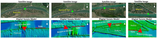
Figure 8.
Rupture scenarios (breaches) in the dykes of the settlements Partizani, Ilganii de Sus, Vulturu, and Maliuc: the upper line of subfigures show the location of the breaches on ortophotomap, second line of subfigures shows the breaches in the dyke on DTM representation.
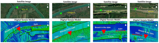
Figure 9.
Rupture scenarios (breaches) in the dykes of the settlements Mila 23, Gorgova, Crișan, and Sulina: the upper line of subfigures show the location of the breaches on ortophotomap, second line of subfigures shows the breaches in the dyke on DTM representation.
Table 2.
The locations of the breaches considered in the dyke.
Based on the river flooding of 6 July 2010, a flow hydrograph of maximum discharge 16,600 m3/s was validated. The hydrological data were completed with information collected from the existing hydrological stations in the Danube Delta. Table 3 presents the maximum water levels from 2010 (with reference to the Black Sea Sulina and the Black Sea 1975) of the Danube near the examined settlements.
Table 3.
Maximum water levels for the year 2010 in meters Black Sea 75 (BS75) and the Black Sea Sulina (BSS) of the Danube near the settlements.
After the boundary conditions were accomplished (upstream: the flow hydrograph and downstream: the normal depth), the process was validated. The input value for the normal depth was 0.04. This value was the energy slope that was used in the software for calculating the normal depth. For this study, the energy slope was approximated by using the average slope of the water surface near the cross-sections. The next stage defined the start and end period of the simulation. Several flow hydrographs were applied in the software, corresponding to the flood stages, to obtain several flood scenarios (32 scenarios in total). The flood stages are presented in Table 4.
Table 4.
Sets of flooding water levels in meters with reference to the Black Sea 75 (BS75) and the Black Sea Sulina (BSS), applied to the settlements.
For each settlement, four flooding stages were applied with intervals between 60 cm and 62 cm (Partizani settlement), 17, 40, and 80 cm (Ilganii de sus), 16 and 60 cm (Vulturu), 38 and 40 cm (Maliuc), 20 and 21 cm (Gorgova), 15 and 40 cm (Mila 23), 20 cm (Crișan), and 9 and 20 cm (Sulina). Flooding stages were presented in the Sulina Black Sea reference system and the Black Sea 75 system. Flooding stages were calculated from the lowest flooding level to the highest flooding level for each analyzed settlement. Thus, different flood scenarios of the settlements for different water levels in the river next to them could be visualized.
In the software, the hydraulic calculations were performed on 06 July 2010 at 10:00, for 24 h (the timeframe in which the flooding breach is maintained in the dyke for the dynamic method). Thus, 32 scenarios were run by execution of the unsteady flow simulator, the pre-processor geometry, and the output post-processor, finally obtaining the results by the first method (dynamic).
The process of hydraulic modeling involves the introduction and use of a large number of data, both geographical and hydraulic [36]. After completing the data entry process and validating the model (including resolving the data entry errors), the program was run and the results of the hydraulic modeling were obtained. The results of hydraulic modeling can be visualized in several ways: maps, graphs, or tables. In the present study the results were displayed in the form of the flooding maps.
For the static method Global Mapper v17.0.2 specialized software was used. Less data were processed with this method than with the previous one. Geographic data, regional boundaries, and orthophotomaps were processed, but mostly the high-resolution digital terrain model. For the correct processing of the information, and to select the study area, the digital terrain model was introduced into the software, and translated into the suitable reference system (STEREO 70, EPSG: 31,700 with the Black Sea 75 system for elevation points). The next step was the individual clipping of the area of interest from the digital terrain model (a sufficiently extensive perimeter was chosen to perform the simulation; this perimeter covered the administrative territorial unit and the adjacent territory for each settlement). The flow area for each settlement was defined by establishing the regional limits (Figure 10).
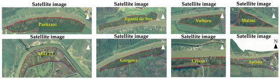
Figure 10.
The boundary representation of the flow surface for each settlements: Partizani, Ilganii de Sus, Vulturu, Maliuc, Mila 23, Gorgova, Crișanand Sulina.
In the next step, using the water rise calculation function, the resolution of the analyzed grid was set to 5 m in both main directions, x and y. This was where the water level increase amounts, using the flooding levels established in Table 4, were also introduced. Thereby, the information corresponding to the maximum levels reached in 2010 (in the Black Sea 75 reference system) was superimposed over the digital terrain model. The application of this method corresponded to the most unfavourable scenario, by maintaining breaches in the flood dyke of settlements for a very long time (more than 24 h). Thus, 32 scenarios were run for the analyzed localities.
The results were generated in the form of flooding maps with flooded areas for each settlement, and were largely based on the digital terrain model.
GIS software was used to adapt these materials to the requirements of the hydraulic modeling software and to the size of the study area. The study area being large, the size of the files used was considerable, which made it difficult to process the data at a later stage, and to introduce geographic data into the specialized software. For the development of the hydraulic model of the Danube Delta, two types of materials were collected as cartographic support. The first type of material included the digital terrain model, and the ortho photomaps of the Danube Delta. The second type of material was less recent, being topographic maps made in 1965. These two materials were refined and processed in the first phase in GIS (ArcMAP 10.4 specialized software), to bring them into the appropriate projection system. The projection used was STEREO 70, with the reference system Black Sea 75 for elevations. Based on these materials, a contour was drawn for the delimitation of the study area, both for the hydraulic modeling and for the GIS analysis. In the case of the hydraulic modeling, the area taken into account spread over the Tulcea and Sulina branches, and in the case of the GIS analysis, the area was limited to the administrative–territorial unit of each settlement on the Sulina branch.
5. Discussion
After running the software, 64 flood scenarios resulted (32 scenarios for each method), and the most relevant results were extracted for the eight settlements from the Danube Delta targeted in the present work. The results were maps illustrating the potentially floodable areas of the analyzed settlements in the Danube Delta. In more detail, the flooding maps obtained in the present study were overview maps that showed, for each flooding level considered, the flood boundary, which represents the extent of the water for each case (scenario) considered, and the depth or water level, depending on the method.
The flooding maps resulting from the application of the dynamic method had a depth class of 0 to 2 m. The flood maps resulting from the static method established the depth as the difference between the considered water level of the flooded surface and the ground level (the elevation of the terrain on the digital terrain model expressed in the Black Sea reference system 75).
In approaching the dynamic method, the hydraulic scenario set was developed using the hydraulic model of the Danube Delta to determine the flood surfaces for each settlement. In both methods, the historical maximum level reached in the summer of 2010 was considered for all localities. The results of applying the maximum level were reflected in the flood–stage IV. Subsequently, to obtain flood scenarios at lower water levels than in 2010, flood stages (Table 4) were applied (the differences being a few centimetres or tens of centimetres from the peak), and so several flooding map scenarios resulted for each settlement analyzed, as presented in Figure 11, Figure 12 and Figure 13. All of these in case of failure of the protective dam. The scenarios in flood stage I corresponded to the lowest level of flooding, while the scenarios in flood stage IV corresponded to the maximum level of flooding, and the scenarios in flood stages II and III corresponded to the intermediate levels of flooding, between the maximum and the lowest level. The most useful way to visualize the results of the hydraulic modeling and GIS processing was with the help of maps, thus being able to refer both to the development in time and in space of the phenomenon. With the help of the hydraulic modeling software, in the first phase, the flood limits (as maps) and the flooding process could be extracted (the scenarios can also be viewed as video). Next, with these results, further processing or interpretation was done in GIS, and other specialized programs.
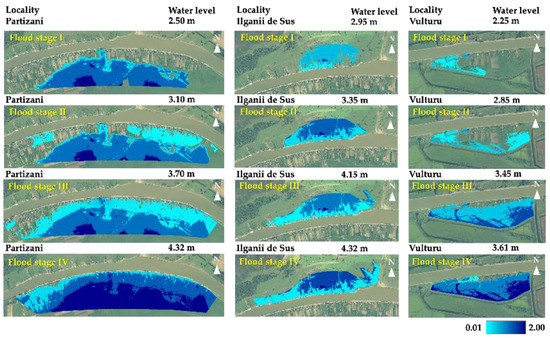
Figure 11.
Flood scenarios maps for Partizani (first column group of subfigures), Ilganii de Sus (second column group of subfigures), and Vulturu (third column group of subfigures) settlements, corresponding to the condition of 7 July 2010, by using the 1D/2D HEC-RAS model, at high resolution DTM 0.5 m × 0.5 m, dynamic method.
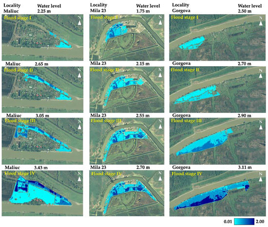
Figure 12.
Flood scenarios maps for Maliuc (first column group of subfigures), Mila 23 (second column group of subfigures), and Gorgova (third column group of subfigures) settlements, corresponding to the condition of 7 July 2010, by using the 1D/2D HEC-RAS model, at high resolution DTM 0.5 m × 0.5 m, dynamic method.
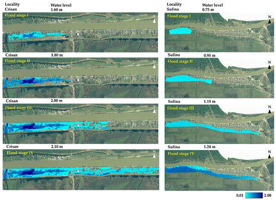
Figure 13.
Flood scenarios maps for Crișan (first column group of subfigures) and Sulina (second column group of subfigures) settlements, corresponding to the condition of 7 July 2010, by using the 1D/2D HEC-RAS model, at high resolution DTM 0.5 m × 0.5 m, dynamic method.
The results were presented by Ras Mapper, using the hydraulic model 1D/2D HEC-RAS at high resolution (DTM 0.5 m × 0.5 m). Figure 11, Figure 12 and Figure 13 present the propagation trend of the flood surface depths over the flooded area, after 24 h from the beginning of the simulation. The elevations used in the data processing with the dynamic method were referenced to the Black Sea 75 system (BS75). The results obtained from the application of the dynamic method identified flooding areas and water depths close to the settlements in the situation of maintaining the breach in the dyke for a period of 24 h.
This method is much more complex than the static method, as it requires a wider range of specific data and knowledge from the operator. If the main concern is to anticipate the current or future behaviour, obtaining relevant field data is an important and integral part of the modeling process [36]. Good results depend on the exact formulation of the problem, and the correct identification of the main parameters that influence the investigated phenomena. Analysing the most unfavorable scenario (flood stage IV-maximum water level), there were several floodable surfaces inside the settlements (Table 5).
Table 5.
The flooded areas of the settlements analyzed at the flood stage IV: maximum water level of the Danube.
For the dynamic method the modeled flooded area was calculated using ArcGIS software. From RAS Mapper–Animator, it was found that the maximum flooded areas at flood stage IV was 5.79 km2 (for all settlements), the simulation taking place between 10:00 of 6 July 2010 and 10:00 of 7 July 2010. The flood surface depth reached up to 1.94 m (flood stage IV Partizani settlement), 1.85 m (flood stage IV Ilganii de Sus), 1.91 m (flood stage IV Vulturu settlement), 1.89 m (flood stage IV Gorgova settlement), 1.66 m (flood stage IV Mila 23 settlement), 1.90 m (Gorgova settlement), 1.95 m (Crișansettlement), and 1.47 m (Sulina settlement).
Figure 12, Figure 13 and Figure 14 indicate that the areas flooded under the four flood stages in the dynamic method, varied between 0.8 km2–1.68 km2 (Partizani), 0.26 km2–0.49 km2 (Ilganii de Sus), 0.80 km2–0.33 km2 (Vulturu), 0.025 km2–0.18 km2 (Maliuc), 0.8 km2–0.71 km2 (Gorgova), 0.21 km2–0.77 km2 (Mila 23), 0.05 km2–0.34 km2 (Crișan), and 0.15 km2–1.29 km2 (Sulina). From the results of the simulations performed we noticed that the flood extension covered households, infrastructure elements, and vacant land in different proportions from one flood stage to another. It can be seen in Figure 11, Figure 12 and Figure 13 that water flows in localities from one zone to another, following the slope of the natural topography. The widespread use and role of hydraulic models have changed in the recent years, mainly due to the significant advances in computer modeling. They remain an important modeling tool, especially in the design of hydraulic, river structures, and coastal engineering applications, as well as for environmental protection, or in providing physical input data for mathematical modeling [46].
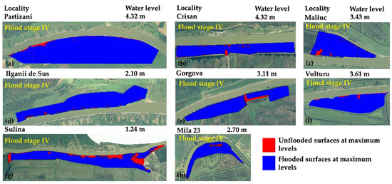
Figure 14.
The representation of digital maps with flooded areas for settlements: (a)—Partizani, (b)—Crișan, (c)—Maliuc, (d)—Ilganii de sus, (e)—Gorgova, (f)—Vulturu, (g)—Sulina, (h)—Mila 23, by using GIS analysis, at high resolution DTM 0.5 m × 0.5 m, static method.
Figure 14 shows the results of the static method. The results are presented in the form of flooding maps that represent the potentially floodable areas of the analyzed settlements in the Danube Delta at flood stage IV (the maximum water level), in the situation of maintaining the breach in the dyke for more than 24 h.
The results obtained following the application of the static method highlight the flood surfaces in the settlements corresponding to the maximum water level of the Danube, this situation being the most unfavorable (the water level on the Danube being the same as the water level in the localities targeted, by keeping the breach in the protective dam for a longer period). This method is less complex than the dynamic method, as it requires a smaller set of specific data and knowledge from the operator. By the analysis of the most unfavorable scenario, floodable surfaces inside the localities resulted, and they are presented in Table 5.
The differences between the two methods are summarized in Table 5. For the static method the flooded area was calculated using Global Mapper software. From the software, it was found that the maximum flooded areas at flood stage IV was 6.51 km2. The flood surface depth reached up to 4.08 m (flood stage IV Partizani settlement), 3.46 m (flood stage IV Ilganii de Sus), 2.85 m (flood stage IV Vulturu settlement), 2.64 m (flood stage IV Gorgova settlement), 2.61 m (flood stage IV Mila 23 settlement), 2.59 m (Gorgova settlement), 2.06 m (Crișansettlement), and 1.65 m (Sulina settlement).
For some settlements the differences were significant, considering that the second method (static) involved maintaining the breach for a long enough time to flood at maximum levels all areas below this level within the settlements. In the case of the first method’s (dynamic) analysis, with 1D/2D hydraulic modeling, the actual flooded surfaces were determined for a shorter period (24 h), resulting in smaller flooded surfaces.
Following the comparative results (applying flooding stage IV-maximum water level), it can be observed that 75% of localities (6 out of 8) had more than 91% of their surface flooded, if the breaches were maintained for more than a day in the dykes of the settlements, and at maximum water levels of the Danube. In the case of maintaining the breaches for a period of only 1 day, it was observed that only one out of eight settlements considered had a flooded area of more than 90%.
In the application of the two methods, for some of the settlements, slightly bigger differences were noticed regarding the flooded surface. The most significant differences appeared for the settlements Vulturu, Crișan, and Sulina, with differences exceeding 12%, and reaching up to approximately 17% in some cases. In order to analyze, in percentage, the differences regarding the flooded areas in all the other flood stages (flood stage I, flood stage II, and flood stage III), some graphs were designed, showing the dynamics of the flooded areas in the scenarios analyzed for the settlements (Figure 15 and Figure 16).
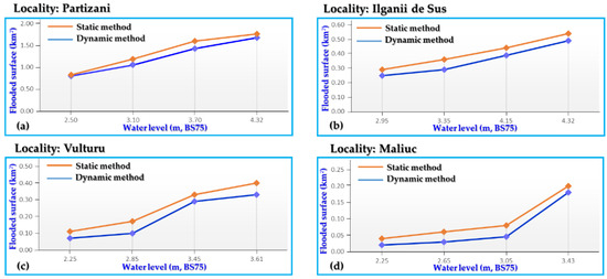
Figure 15.
The differences of flooded area for the analyzed scenarios by using static method and dynamic method at: (a)—Partizani, (b)—Ilganii de Sus, (c)—Vulturu, and (d)—Maliuc settlements.
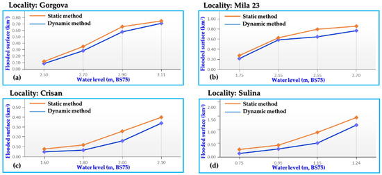
Figure 16.
The differences of flooded area for the analyzed scenarios by using static method and dynamic method at: (a)—Gorgova, (b)—Mila 23, (c)—Crisan, and (d)—Sulina settlements.
The dynamics of the flooded areas for the analyzed settlements differed from one method to the other. From the displayed results, it is visible that by applying the static method in all flood stages, the flooded surfaces were larger compared to the flooded surfaces obtained by applying the dynamic method.
Figure 15 and Figure 16 indicate that the areas flooded under the four flood stages in the static method, varied between 0.85 km2–1.76 km2 (Partizani), 0.29 km2–0.54 km2 (Ilganii de Sus), 0.11 km2–0.40 km2 (Vulturu), 0.04 km2–0.20 km2 (Maliuc), 0.11 km2–0.75 km2 (Gorgova), 0.23 km2–0.86 km2 (Mila 23), 0.08 km2–0.40 km2 (Crișan), and 0.28 km2–1.60 km2 (Sulina).
Referring to the first flood stage, the largest percentage differences between the two methods regarding the flooded area were observable for Vulturu (difference of 9.63%) and Maliuc (difference of 9.17%). The smallest percentage differences in the first flood stage were observable for Partizani (difference of 1.68%) and Gorgova (difference of 3.68%). For the second flood stage, the largest percentages, in terms of the differences regarding the flooded area, appeared in Ilganii de Sus (difference of 12.55%), Vulturu (difference of 16.85%), Maliuc (difference of 13.76%), and Crișan (difference of 10.44%), and the smallest difference was found in Mila 23 (difference of 4.30%). In the third flood stage, the largest percentage differences regarding the flooded area were recorded in the settlements of Crișan (difference of 21.89%) and Sulina (difference of 21.20%). At the same time, the smallest percentage differences were present in Partizani (difference of 9.46%), Ilganii de Sus (difference of 8.96%), Vulturu (difference of 9.63%), and Gorgova (difference of 9.83%).
The dynamic method gives the lowest percentage of flooded areas for all the settlements. This is due to the fact that the dynamic method involves flooding the surfaces gradually, and depending on the topography of the terrain. Gradual surface flooding is induced by the flow of the river, and so the area flooded by considering the dynamic method at water levels such as those shown in flood stages II and III, was smaller than the area flooded by considering the static method. In addition to this fact, the physical–geographical factors had a certain influence on the process of flood leakage in the dynamic method. Here the relief influences the size, and especially the distribution, of the flood leakage by its degree of fragmentation and by the size of the slope of the land in the localities considered. If we analyze the evolution of the flood at all flood stages, in Figure 11 and Figure 12 we can see that the flooded area increased sharply in the localities Vulturu (from 0.10 km2 in flood stage II to 0.29 km2 in flood stage III), and Maliuc (from 0.04 km2 in flood stage III to 0.18 km2 in flood stage IV). In the case of the settlements Partizani and Ilganii de Sus, the flooded area showed a constant increase in all flood stages. This was due to the fact that the land surface tends to a smoother slope compared to Vulturu and Maliuc settlements, where the slope in some areas becomes steep. At the same time there are other factors that influenced the process of flood leakage in the dynamic method, such as vegetation, which has an important role in the leakage process. On one hand by influencing the soil formation, and on the other hand contributing to increasing capacity of infiltration in the soil and reducing soil erosion. Another important factor is the land use. This essentially and negatively influences flood leakage conditions. Furthermore the anthropic factor has an important role on the formation of flood leakage, specifically through the changes brought to the natural system: the change of the land cover (natural vegetation was replaced by agricultural crops (the most common case in the Danube Delta), orchards, vineyards, and human settlements), and changes to the Danube riverbed to ensure the necessary water (for irrigation, water needs, electricity, construction materials, etc.), road networks, flood protection works, etc. As a result of the increasing intervention of man in the natural systems, their natural evolution is disturbed, the changes being significant or fundamental. In the latter case, the intervention causes breaks in the rhythm of the natural development, imbalances that accentuate the involution of the respective landscapes. The comparative analysis of the results highlighted, first of all, the substantial effect of reducing the flooded areas, at a lower flood level of the Danube, with differences from one settlement to another. The flooding maps for the analyzed settlements provide information on the extent of floodable areas and the depth of the water in several flooding stages. We examined flood scenarios in the event of a breach occurrence in a settlement’s dyke during a heavy river flooding to investigate the impact on the study area in terms of flooded surfaces, using two methods. We also took into account the 2010 Danube flood, relying on hydrological data (records at the Tulcea-port hydrometric station that produced daily data, and data provided by the Danube Delta National Institute for Research and Development, and the Romanian Waters National Administration).
Using GIS, the processing of this data could be done much faster and easier, and in a much more accessible interface. The use of GIS is essential in flood scenario analysis; throughout the process, from its initiation to the interpretation phase. The GIS systems were used to facilitate the visualization of the study area, and to enter, refine, and process the hydrological data needed in the flood scenario analysis, as well as to interpret the results, and to present them as comprehensively as possible. In order to choose the most appropriate flood analysis model, it is necessary to have access to geographical information that can provide an overview of the components of the water circulation system [47]. High resolution digital terrain models are decisive for the precise output of flood stages and flooded surfaces. Table 6 presents a comparative analysis of the analysis methods used in this work, taking into account the software options.
Table 6.
Comparative analysis of the analysis methods used.
6. Conclusions
In the Danube Delta, floods are hydrological events that can occur at any scale, and it has been noticed that they have appeared more often in the last decades. Flooding is influenced by the rate of the Danube water level rise. Depending on their magnitude, they proportionally affect a certain part of the Delta area, and especially the settlements along the main branches of the river.
From this perspective, the analysis of two different scenarios considering the breaching of the dyke for localities along the Sulina branch of the Danube River was performed in the present work. The study was carried out using a dynamic method of hydraulic modeling, and a static method of GIS analysis, to identify the flooding maps for different scenarios.
An important conclusion was derived from the topo-bathymetric measurements. To achieve the main purpose of this study, it was important to develop a good DTM, by improving the LIDAR model with minor river bathymetry. The digital model of the minor river bed, coupled with the digital terrain model for the Danube Delta allowed the simulation of more flooding scenarios for the localities, and considering various flooding tests.
Furthermore, it can be mentioned that the results of hydraulic modeling, in case of dynamic modeling, are directly influenced by the coefficient of roughness (Manning’s roughness coefficient), which in this study ranged between 0.025 and 0.03. According to Chow [48], these Manning values are specific to natural minor streams; clean, straight, full stage, no rifts, or deep pools.
Furthermore, the results of the hydraulic model were validated by using real data. This revealed the effectiveness of the model in identifying areas prone to floods.
The results showed that for the first breaking scenario of the dyke (the dynamic method) the flooded areas covered a smaller area than in the case of the second scenario (the static method), when the flooded zones covered a considerably larger area. The most significant differences were noticed for the localities Vulturu, Crișan, and Sulina. The results obtained also revealed the flooded surface in percentage and the expected water depth in each locality studied. The increase of the Danube levels led to a gradual increase of the flooded surface inside the localities, in the case of a breach in the dyke. The accuracy of the model simulations depends to a large extent on the accuracy of the DTM, the hydrological and hydraulic structure of the model, and the characteristics of the soil.
Finally, it can be concluded that floods caused by high water levels or by dam failure can be analyzed through a combination of 1D/2D techniques or through a GIS analysis. The emphasis was on comparison of flooded surfaces resulting from the two methods.
The static method used with the help of Global Mapper software does not require so much data and knowledge from the operator as the dynamic method. The second method requires complex data and information for the elaboration of a hydraulic model in HEC-RAS for a 1D/2D simulation (field data, hydraulic parameters, flows, levels, types of graphical representation, networks, nodes, conditions of margin). The use of the static method in performing flood simulations does not require topo-bathymetric data like the dynamic method, which results in the fact that the static method is exempt from the time and effort allocated to perform field measurements. At the same time, the disadvantage of the static method is that the simulations cannot be calibrated with field data. The dynamic methodology has the advantage of introducing a much more complex input data set, including calibration data, which gives a higher confidence in the results obtained. From the comparison presented in Table 6 and the results obtained from the simulations, it can be seen that both methods give similar results regarding the flooded area, the differences being outlined in the percentage of coverage of the flooded area in the localities. However, the dynamic method is much more realistic compared to the static method, due to the multiple advantages that the HEC-RAS program has, such as: multiple functions and options, choice of simulation period, facilities related to setting initial and boundary conditions, facilities related to the flow slope, etc.
The approach of 1D/2D hydraulic modeling techniques is more realistic compared to the static method, taking into account the fact that the real flooded areas were determined for different scenarios of dyke breach with a duration of 24 h (the time of maintaining the breach), which could allow a real estimate of the material and human resources needed to intervene in an emergency. The approach with several scenarios allowed the testing of the water flow capacity in the settlements, determining to what extent the surfaces inside the settlements would be affected. The area targeted, located in the Danube Delta, presents an elevated danger of inundations.
The novelty of this work is based on showing different complex techniques how can be used to assess flood extent by apply two different flood simulation methods. At the same time the used methods represent a low to medium cost solution, by which flood maps can be generated in previously unassessed areas.
The purpose of the flooding maps is to support decision making, the elaboration of flood management plans, public awareness, or other activities of general interest. Furthermore, the analysis performed is important, and there is a huge potential for the development of a robust approach in other similar situations for any type of area.
Last but not least, ideas for a new research work were derived from this paper, entailing the use of the results in order to assess the possible flood risk and hazard for all the presented localities. In this case repeated in situ bathymetric measurements will be done, in order to assess the spatial-temporal differences, and to obtain an updated hydrological model.
Author Contributions
A.B. processed the numerical data, designed the figures and tables and wrote the first form of the manuscript, C.I. contributed to the interpretation of the results and L.P.G. supervised the work. E.R. and M.A. performed the literature review, corrected the manuscript and acted as corresponding author. All authors have read and agreed to the published version of the manuscript.
Funding
This work was supported by the project “EXPERT”, financed by the Romanian Ministry of Research and Innovation, Contract No. 14PFE/17.10.2018.
Acknowledgments
This work was supported by the project “Excellence, performance and competitiveness in the Research, Development and Innovation activities at “Dunarea de Jos” University of Galati”, acronym “EXPERT”. This work was financed by the Romanian Ministry of Research and Innovation in the framework of Program 1—Development of the national research and development system, Sub-program 1.2—Institutional Performance—Projects for financing excellence in Research, Development and Innovation, Contract No. 14PFE/17.10.2018. The authors would like also to express their gratitude to the reviewers for their valuable suggestions and observations that helped in improving the present work.
Conflicts of Interest
The authors declare no conflict of interest.
Appendix A

Figure A1.
Graphs with monthly distribution of the minimum and maximum water levels of the Danube at the Tulcea hydrometric station in 2003 and 2010. (a) Monthly frequency of the minimum water levels; (b) monthly frequency of the maximum water levels; (c,e) graphs with normalized values corresponding to the monthly frequency of the minimum water levels; (d,f) graphs with normalized values corresponding to the monthly frequency of the maximum water levels.

Figure A2.
The digital terrain model for the Danube Delta superimposed on the orthophotomaps (the red dots indicate the settlements located along the Sulina branch.

Figure A3.
Bathymetric cross-section profiles (magenta lines) and bank points (yellow dots), measured for S1 (a), S2 (b), and S3 (c), sections of the study area. The third line subfigures (d–f) represents the combined 3D model obtained from LIDAR and bathymetric data for all three sections of the study area.

Figure A4.
Longitudinal profile of the main channel of all three sections from study area: (a–c)—the plane view of longitudinal river centerline of S1, S2 and S3 cross-section path; (a1–c1)—section view for the depth profiles of centerline at S1, S2 and S3 river part.

Figure A5.
Rating curve values at the Tulcea gauge station during the 2010 flood year.
References
- Tincu, R. Evaluation of the Risk Produced by Floods on the Trotus River the Section Afferent to Ghimes—Faget Locality Using Geographic Information Systems (GIS). Ph.D. Thesis, Vasile Alecsandri University of Bacau, Bacau, Romania, 2018. [Google Scholar]
- Arseni, M.; Roșu, A.; Bocăneală, C.; Constantin, D.-E.; Georgescu, P.L. Flood hazard monitoring using GIS and remote sensing observations. Carpathian J. Earth Environ. Sci. 2017, 12, 329–334. [Google Scholar]
- Sageata, R.; Dumitrescu, B. Typologies of urban vulnerability to flooding in Romania. J. Wulfenia 2013, 11, 274–290. [Google Scholar]
- Radulescu, D.; Ion, M.; Chendes, V. Preliminary flood risk assessment on the Romanian territory. J. Rom. Assoc. Hidro Sci. 2013, 8, 14–19. [Google Scholar]
- Beltaos, S. The 2014 ice–jam flood of the Peace-Athabasca Delta: Insights from numerical modelling. Cold Reg. Sci. Technol. 2018, 155, 367–380. [Google Scholar] [CrossRef]
- Nones, M.; Maselli, V.; Varrani, A. Numerical modeling of the hydro-morphodynamics of a distributary channel of the po river delta (Italy) during the spring 2009 flood event. Geosciences 2020, 10, 209. [Google Scholar] [CrossRef]
- Win, K.T.; Aye, N.; Htun, K.Z. Vulnerability of Flood Hazard in Selected Ayeyarwady Delta Region, Myanmar. Int. J. Sci. Eng. Appl. 2014, 3, 44–48. [Google Scholar] [CrossRef]
- Molina, J.L.; Rodríguez-Gonzálvez, P.; Molina, M.C.; González-Aguilera, D.; Espejo, F. Geomatic methods at the service of water resources modelling. J. Hydrol. 2014, 509, 150–162. [Google Scholar] [CrossRef]
- Zazo, S.; Molina, J.L.; Rodríguez-Gonzálvez, P. Analysis of flood modeling through innovative geomatic methods. J. Hydrol. 2015, 524, 522–537. [Google Scholar] [CrossRef]
- Gergel’ová, M.B.; Kuzevičová, Ž.; Labant, S.; Gašinec, J.; Kuzevič, Š.; Unucka, J.; Liptai, P. Evaluation of selected sub-elements of spatial data quality on 3D flood event modeling: Case study of Prešov city, Slovakia. Appl. Sci. 2020, 10, 820. [Google Scholar] [CrossRef]
- Mierlă, M.; Romanescu, G. Hydrological flood risk assessment for Ceatalchioi locality Danube Delta. Geogr. Sem. Dim. Cantemir 2013, 6, 11–22. [Google Scholar]
- Poncos, V.; Teleaga, D.; Bondar, C.; Oaie, G. A new insight on the water level dynamics of the Danube Delta using a high spatial density of SAR measurements. J. Hydrol. 2013, 482, 79–91. [Google Scholar] [CrossRef]
- Romanescu, G.; Stoleriu, C.C. Anthropogenic interventions and hydrological-risk phenomena in the fluvial-maritime delta of the Danube (Romania). Ocean Coast Manag. 2014, 102, 123–130. [Google Scholar] [CrossRef]
- Panin, N. The Danube Delta—The mid term of the geo-system Danube River—Danube delta—Black Sea. Rom. J. Geol. 2011, 55, 41–82. [Google Scholar]
- Stan, N.; Enache, N. The Crisis Situation Management and of the Emergencies Situation; National Agency Civil Servants: Rome, Italy, 2013.
- Banescu, A.; Georgescu, L.; Iticescu, C.; Rusu, E. Analysis of the flood risk in the Danube Delta—Case study: The Maliuc area. Ann. Univ. Dunarea Jos Galati. 2018, 41, 40–47. [Google Scholar]
- Armasae, I.; Armasae, A.; Avram, E. Perception of flood risk in Danube Delta, Romania. Nat. Hazards 2009, 50, 269–287. [Google Scholar] [CrossRef]
- Banescu, A.; Georgescu, L.; Rusu, E.; Murariu, G. Analysis of the floods risk in the peripheral localities from the north of the Danube Delta using GIS technologies. In Proceedings of the International Multidisciplinary Scientific GeoConference, Albena, Bulgary, 28 June 2019; pp. 723–732. [Google Scholar]
- Bajo, M.; Ferrarin, C.; Dinu, I.; Umgiesser, G.; Stanica, A. The water circulation near the Danube Delta and the Romanian coast modelled with finite elements. Cont. Shelf Res. 2014, 78, 62–74. [Google Scholar] [CrossRef]
- Munteanu, I.; Tuzlaru, C.; Arefi, N.; Cioroiu, L.; Raileanu, G.; Bascau, F.; Nițu, M. Raport Privind Starea Mediului in Rezervatia Biosferei Delta Dunarii in Anul 2015 (Report on the State of the Environment in the Danube Delta Biosphere Reserve); Danube Delta Biosphere Reservation Administration: Tulcea, Romania, 2015. [Google Scholar]
- Popescu, I.; Lericolais, G.; Panin, N.; Normand, A.; Dinu, C.; Le Drezen, E. The Danube submarine canyon (Black Sea): Morphology and sedimentary processes. Mar. Geol. 2004, 206, 249–265. [Google Scholar] [CrossRef]
- Banescu, A.; Georgescu, L.; Rusu, E.; Murariu, G. Analysis of the floods risk in a sector from the Danube Delta using GIS technologies. In Proceedings of the 18th International Multidisciplinary Scientific GeoConference, Albena, Bulgary, 2 July 2018; pp. 307–314. [Google Scholar]
- Armas, I.; Ionescu, R.; Posner, C.N. Flood risk perception along the Lower Danube river, Romania. Nat. Hazards 2015, 79, 1913–1931. [Google Scholar] [CrossRef]
- Demir, V.; Kisi, O. Flood Hazard Mapping by Using Geographic Information System and Hydraulic Model: Mert River, Samsun, Turkey. Adv. Meteorol. 2016, 2016, 4891015. [Google Scholar] [CrossRef]
- Brakenridge, G.R.; Andersona, E.; Nghiemb, S.V.; Caquard, S.; Shabaneh, T.B. Flood Warnings, Flood Disaster Assessments, and Flood Hazard Reduction: The Roles of Orbital Remote Sensing; Jet Propulsion Laboratory, National Aeronautics and Space Administration: Pasadena, CA, USA, 2003.
- Cioaca, E. Morphohydrographic Evolution of the Danube Delta Biosphere Reserve Zones Subject to the Ecological Reconstruction Process; Scientific Annals Danube Delta Institute for Research and Development: Tulcea, Romania, 2001. [Google Scholar]
- Gâştescu, P. The Danube Delta Biosphere Reserve Geography biodiversity protection management. Rom. J. Geogr. 2009, 53, 139–152. [Google Scholar]
- Rusu, E. Modelling of wave-current interactions at the mouths of the Danube. J. Mar. Sci. Technol. 2010, 15, 143–159. [Google Scholar] [CrossRef]
- EcoPotential Project. (n.d.). Danube Delta. Available online: https://ecopotential-project.eu/site-studies/protected-areas/33-danube-delta (accessed on 11 November 2020).
- Gómez-Baggethun, E.; Tudor, M.; Doroftei, M.; Covaliov, S.; Năstase, A.; Onără, D.F.; Mierlă, M.; Marinov, M.; Doroșencu, A.-C.; Lupu, G.; et al. Changes in ecosystem services from wetland loss and restoration: An ecosystem assessment of the Danube Delta (1960–2010). Ecosyst. Serv. 2019, 39, 100965. [Google Scholar] [CrossRef]
- Bondar, C.; State, I.; Cernea, D.; Harabagiu, E. Water flow and sediment transport of the Danube at its outlet into the Black Sea. Met. Hydrol. 1991, 21, 21–25. [Google Scholar]
- Panin, N.; Jipa, D. Danube river sediment input and its interaction with the north-western Black Sea. Estuar. Coast. Shelf Sci. 2002, 54, 551–562. [Google Scholar] [CrossRef]
- Niculescu, S.; Lardeux, C.; Hanganu, J.; Mercier, G.; David, L. Change detection in floodable areas of the Danube delta using radar images. Nat. Hazards 2015, 78, 1899–1916. [Google Scholar] [CrossRef]
- Cioaca, E.; Bondar, C.; Borcia, C. Hydrographical network of the Danube Delta Biosphere Reserve-modelling the morphological dynamics. In Proceedings of the 38th IAD Conference, Dresden, Germany, 22–25 June 2010; pp. 1–5. [Google Scholar]
- Pleniceanu, V.; Ionus, O.; Licurici, M. Extreme hydrological phenomena in the hydrographical basin of the Danube. The floods from the spring of 2006 along the oltenian sector of the river. Ann. Univ. Craiova Ser. Geogr. 2008, 11, 37–47. [Google Scholar]
- Grimaldi, S.; Petroselli, A.; Arcangeletti, E.; Nardi, F. Flood mapping in ungauged basins using fully continuous hydrologic-hydraulic modeling. J. Hydrol. 2013, 487, 39–47. [Google Scholar] [CrossRef]
- Bakuła, K.; Stȩpnik, M.; Kurczyński, Z. Influence of Elevation Data Source on 2D Hydraulic Modelling. Acta Geophys. 2016, 64, 1176–1192. [Google Scholar] [CrossRef]
- Watts, S.; Halliwell, L. Essential Environmental Science—Methods And Techniques, 1st ed.; Routledge: New York, NY, USA, 1996. [Google Scholar]
- Reutebuch, S.E.; Mc Gaughey, R.J.; Andersen, H.E.; Carson, W.W. Accuracy of a high-resolution lidar terrain model under a conifer forest canopy. Can. J. Remote Sens. 2003, 29, 527–535. [Google Scholar] [CrossRef]
- Andrita, M.; Cioaca, C. LIDAR technology usage within forensic science/Aplicatiile tehnologiei LIDAR în tehnica criminalistica. Forum Crim. 2015, 8, 27. [Google Scholar]
- Demarchi, L.; Bizzi, S.; Piégay, H. Regional hydromorphological characterization with continuous and automated remote sensing analysis based on VHR imagery and low-resolution LiDAR data. Earth Surf. Process Landf. 2017, 42, 531–551. [Google Scholar] [CrossRef]
- Nichersu, I.; Mierla, M.; Trifanov, C.; Nichersu, I.; Marin, E.; Sela, F. Digital Cartographic Models as Analysis Support in Multicriterial Assessment of Vulnerable Flood Risk Elements; EGU General Assembly Conference: Viena, Austria, 2014; Volume 16. [Google Scholar]
- Harman, B.I.; Koseoglu, H.; Yigit, C.O. Performance evaluation of IDW, Kriging and multiquadric interpolation methods in producing noise mapping: A case study at the city of Isparta, Turkey. Appl. Acoust. 2016, 112, 147–157. [Google Scholar] [CrossRef]
- Arseni, M.; Voiculescu, M.; Georgescu, L.P.; Iticescu, C.; Rosu, A. Testing Different Interpolation Methods Based on Single Beam Echosounder River Surveying. Case Study: Siret River. ISPRS Int. J. Geo-Inf. 2019, 8, 507. [Google Scholar] [CrossRef]
- Arseni, M.; Rosu, A.; Calmuc, M.; Calmuc, V.A.; Iticescu, C.; Georgescu, L.P. Development of flood risk and hazard maps for the lower course of the Siret River, Romania. Sustainability 2020, 12, 6588. [Google Scholar] [CrossRef]
- Cioc, D.; Anton, A.; Georgescu, A. Determination by Calculation of the Optimal of the Optimal Endowment of a Capture Front; UTCB Bucharest Publishing House: Bucharest, Romania, 1999. [Google Scholar]
- Gül, G.O.; Harmancioǧlu, N.; Gül, A. A combined hydrologic and hydraulic modeling approach for testing efficiency of structural flood control measures. Nat. Hazards 2010, 54, 245–260. [Google Scholar] [CrossRef]
- Chow, V.T. Open-Channel Hydraulics; McGraw-Hill College: New York, NY, USA, 1959. [Google Scholar]
Publisher’s Note: MDPI stays neutral with regard to jurisdictional claims in published maps and institutional affiliations. |
© 2020 by the authors. Licensee MDPI, Basel, Switzerland. This article is an open access article distributed under the terms and conditions of the Creative Commons Attribution (CC BY) license (http://creativecommons.org/licenses/by/4.0/).