Abstract
This work is devoted to preliminary numerical tests of selected control strategies of underwater vehicles in the absence of a force applied to the side. The aim was to test the effectiveness of control algorithms for underwater vehicle models considered to be underactuated. Initially, the testing algorithm is used to obtain some information about the dynamics model. Several well-known control schemes for two underwater vehicles for two desired trajectories were selected and tested. The simulations made for the planar 3-DOF model of two underwater vehicles show the performance that can be achieved with each control algorithm according to the assumptions made.
1. Introduction
The control of autonomous underwater vehicles (AUVs) is a complex problem mainly due to the nonlinear dynamics, uncertainty in model parameters, and external disturbances. The AUVs are applied to inspections, surveillance, maintenance, and security within the maritime industry. Due to the availability of forcing signals, these vehicles can be divided into fully actuated and underactuated.
In this work, the problem of the application of known methods of trajectory tracking for underactuated underwater vehicles which move in the horizontal plane is considered. There exist many control schemes that have been applied to this class of vehicles. Various types of control strategies which are suitable for underactuated vehicles may be recalled here.
One method is the Lapunov-based approach which has proven to be useful for the trajectory tracking of marine vehicles [1,2,3] or hovercrafts [4]. A lot of work has been done to solve the problem of trajectory tracking for underactuated AUVs, namely using the backstepping method [5,6,7,8] or backstepping and Lyapunov’s direct methods [9]. The backstepping techniques were employed to realize the trajectory tracking of underactuated ASVs many times. In the traditional approach, however, a serious disadvantage is the computational complexity. Despite this difficulty, this type of technique can be found in [10]. Combinations of this approach with other methods are also available, e.g., in [11] (backstepping and sliding mode control (SMC) method), [12] (averaging and backstepping), ref. [13] (backstepping and integral SMC). Another approach is the output-feedback [14,15], sometimes together with backstepping [14]. Sliding mode control (SMC) is also an effective nonlinear control technique which is characterized by low sensitivity to systematic uncertainty and good disturbances rejection. There are various kinds of this strategy [16,17]. However, some authors suggest modifications of the SMC method to achieve greater precision in tracking trajectories or other benefits [18,19]. Sometimes the terminal sliding mode control (TSMC) method is considered better than the conventional sliding mode control technique (taking into account the finite-time convergence and high steady state tracking precision) and is proposed, e.g., in [18]. The proportional-integral-derivative sliding mode control (PID-SMC) [19] guarantees global convergence and boundedness of all tracking errors in the finite time. Quite different groups of methods but with significant application are strategies based on neural network (NN) learning, e.g., in [20,21,22,23,24]. These methods also include a controller that is a combination of different algorithms, e.g., [23,25] (NN,SMC). Fuzzy logic approach, due to its simple control structure, easy, and cost-effective design, is also employed to the application of underactuated AUVs control. The following works may be mentioned here [26,27]. A review of applications is given in [28]. Another strategy consists of a combination of artificial intelligence, learning with other techniques as it was shown in [29]. Less often, however, other trajectory tracking methods are used as, e.g., prescribed performance [30,31], model predictive control (MPC) [32,33], input-output linearization [34], linear algebra approach [35], and modified dynamic inversion [36]. Valuable works comparing known control algorithms can be found in the literature, e.g., [37]. Since such works have a defined goal, consequently also the research has a limited scope. Of course, for the purposes of initial design verification, known algorithms dedicated to horizontally moving vehicle’s underwater vehicle control can be applied.
The aim of the work was to show some preliminary numerical tests of selected known control algorithms that perform the task of tracking two set trajectory types for arbitrarily adopted two underactuated underwater vehicle models. This test is based on the assumption that the selection of controller parameters should be intuitive (manual or otherwise by trial and error) to avoid the use of additional methods. That is why only such algorithms were chosen for which the intuitive selection of parameters in the source work turned out to be sufficient and there was no mention of the use of an additional selection method or an optimization method. Moreover, a concept of a testing algorithm which gives an insight into the vehicle dynamics is considered. In the limited research, it is interesting to find a potential application of some selected control algorithms suitable for trajectory tracking of underactuated underwater vehicles moving horizontally. Inspiration for considering such a problem is the emerging need to use an appropriate control algorithm that guarantees acceptable tracking results for a desired trajectory. When the model of the underwater vehicle is known and our task is to use the controller to track the desired trajectory one can do two ways: develop our own control scheme or adapt one or more of the control algorithms known from the literature. This work is devoted to this second issue only. For this purpose, a comparison among the control algorithms developed in [4,17,18], and [11] is shown. The first strategy [4] serves for control of an underactuated hovercraft and it is here used as tester for further investigation. The others are intended originally for control of marine vehicles. All algorithms are applied to the control of two selected vehicles treated as underactuated. The other three strategies, i.e., considered in [11,17,18], are various kinds of the sliding mode control.
The proposed approach is particularly important before undertaking research on the usefulness of control algorithms already at the simulation verification stage. At this stage, it is necessary to decide whether it is worth carrying out an experiment on a real object using the selected controller.
The originality of the proposed work can be stated as follows:
- (i)
- the use of a simple test of algorithms which give an insight into the dynamics of the vehicle and control performance;
- (ii)
- to verify in simulation the selected control algorithms appropriate for underactuated underwater vehicles in which gain coefficients are chosen without any additional optimization methods and to show their performance;
- (iii)
- to compare the simulation results obtained for the linear and sine trajectory and for two models of the vehicle.
This work is organized in the following way. In Section 2, the equations of motion used here are given. In Section 3, the selected tracking control algorithms are described shortly. In Section 4, simulations are presented for two different underwater vehicles to demonstrate the effectiveness of each control scheme. Finally, conclusions are made in Section 5.
2. Underwater Vehicle Equations of Motion
The vehicles selected for testing are known from the literature. The vehicle ROPOS, e.g., was described in [38] and Kambara in [14,39]. In this work, the horizontal motion is taken into account and the models are assumed as describing the underactuated vehicles.
The underwater vehicle model moving in the horizontal plane is given in Figure 1.
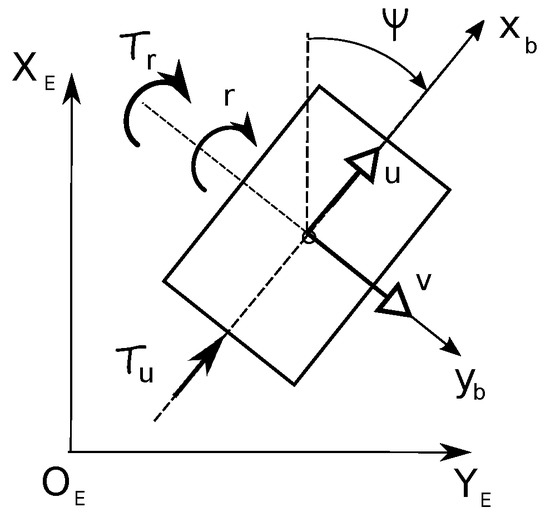
Figure 1.
Underwater vehicle model sketch.
Two types of equations of motion are considered because the first describes a marine vehicle and the second relates to a hovercraft or rudder equipped underwater vehicle. The main goal was to choose from among several control algorithms those that are effective for trajectory tracking. Moreover, there are only preliminary investigations of the selected algorithms. Therefore, it was assumed that the friction forces are omitted which leads to simplification of the vehicle model. For the same reason, the research concerns only a few selected algorithms.
2.1. Model of the 3-DOF Vehicle
The full model of the vehicles considered in this work can be found in [38] (for ROPOS) and in [14,39] (for Kambara). The reduced equations of motion (in the horizontal plane) for an underactuated vehicle used, e.g., in [6,11,36], can be written as follows:
where , are the surge force and the yaw torque, respectively. Moreover, mean the vehicle velocities, and the vehicle position in the inertial frame. The other symbols denote , , and (the mass and the appropriate added mass). In Equations (4)–(6), are linear velocities, r is angular velocity, m is the mass, J is the inertia, , , , are the drag coefficients (with sign + [11] or − [17,18]). The quadratic drags are omitted to enable the comparison of algorithms under the same conditions. The disturbances are not taken into account because of the assumption that it is an the preliminary investigation of algorithms. The equations of motion are assumed in the form which enables comparison of the selected controllers. However, in the second part of this work, the disturbances are taken into account but only for control schemes which gave acceptable results in the first part of the test.
2.2. Testing Model
For the dynamic testing, a different model is considered, namely one that is suitable for a hovercraft [4]. As a result that an underactuated underwater vehicle is investigated, the modified equations replacing (4)–(6) are taken into account:
where is input scaling coefficient, T is the thrust force, a is the length of the arm from center of mass to the rudder surface, and J is the hovercraft inertia. Several issues must be clarified. Since the mass (for hovercraft), then the average value is taken into consideration. Equations (7)–(9) cannot be derived from (4)–(6) because they describe a vehicle of a different design, namely one equipped with a rudder. After modification (neglecting friction), (7)–(9) have slightly different form than in reference [4]. Note also that the forces and the torque are defined differently. Moreover, the equations arise from the design in which both the thrust and the rudder are present. These simplifications are accepted for preliminary test only when it is important to know the movement of the vehicle which is related to its dynamics together with the control algorithm. Some underwater vehicles are equipped with a rudder, e.g., LAUV considered in [34] which suggests that the above-mentioned algorithm may be qualified for the test.
3. Short Description of Selected Algorithms
As a result that the mathematical model of the vehicle is already known, one can attempt to implement the control task for underwater vehicles moving horizontally.
3.1. Various Approaches to Trajectory Tracking
In order to compare usefulness of various control strategies, it is necessary, at the beginning, to mention different approaches to trajectory tracking problem for underwater vehicles. Due to the fact that some methods cannot be clearly classified into one group and also due to the popularity of some methods of trajectory tracking, the division into groups of methods given below is rather a suggestion.
- Lyapunov theory-based methods [1,2,3,4].
- Backstepping (including SMC, output feedback control, Lyapunov method, and others) [5,6,7,8,9,10,11,12,13,14,40].
- Sliding mode control (SMC)-based approaches [16,17,18,19].
- Neural network-based control algorithms and its combination [20,21,22,23,24,25,41].
- Fuzzy control-based methods [26,27].
- Other solutions, e.g., prescribed performance [30,31], input-output linearization [34], linear algebra approach [35], modified dynamic inversion [36], and model predictive control (MPC) [32,33,42].
The methods of the first group are well-known but often they are used together with the backstepping techniques to obtain better mathematical results or controller performance. The disadvantage of this type of method, however, is very accurate knowledge of the dynamic parameters of the vehicle are needed, which is usually difficult to obtain. The second group, namely approaches using backstepping, lead to reliable and effective controllers and they are easy to understand and implement. Many algorithms need output errors to satisfy constraint requirements to avoid singularity. Additionally, the traditional backstepping method caused complexity. Combinations of this method and other approaches are used to reduce the disadvantages of the control strategy. The third group, i.e., schemes based on SMC, is effective for the AUV trajectory tracking controllers. These techniques offer low sensitivity to uncertainty and good disturbance rejection. The methods have difficulties in solving the chattering associated with SMC. Neural networks control (the fourth group), especially adaptive, is one of the tools for improving the tracking performance of AUVs. However, the control schemes are often combined with other types of methods based on a different mathematical approaches, which is a considerable difficulty. In addition, learning of the neural networks is time consuming because the approach heavily depends on the NN nodes. Fuzzy control (the fifth group) is another effective solution to deal with uncertainties. It has been employed many times for application of control in robotics due to its simple structure and because of the easy implementation. Controllers designed for fuzzy systems depend strongly on the number of the fuzzy rule bases, resulting in computational effort. In spite of that, NN or fuzzy-based approaches are very useful for the control of nonlinear dynamics. The methods collected in the sixth group are less popular although they also lead to effective solutions for the trajectory tracking.
3.2. Selected Trajectory Tracking Methods
Since there are many strategies for controlling underactuated underwater vehicles that move horizontally, some selection had to be made based on assumptions.
Assumptions for control schemes selection and test conditions. The method of choosing a control scheme for preliminary tests (1.)–(3.) and the test conditions (4.)–(6.) is as follows:
- the controller was verified at least on simulation using the vehicle parameters given in the original work;
- the control algorithm provides complete information necessary for simulation verification;
- in this preliminary test, the linear and sine desired trajectories and vehicles ROPOS and Kambara are used only;
- the disturbances and other inaccuracies are not taken into consideration in the first test, but in the additional test (done only for algorithms which gave acceptable results in the first part of the test) the disturbances occur;
- only a simple method for selecting control gains is allowed, i.e., the trial and error method; the use of additional searching algorithms is unacceptable.
Comment. The above assumptions were based on the rule that if simulation studies of an algorithm do not produce acceptable results, they also do not guarantee their practical application. On the other hand, selecting the control algorithms for the test was guided by the fact that the source work shows that no additional methods of optimal selection of gain coefficients are necessary, even in the case when these parameters are numerous.
Taking into account the above assumptions and remarks, five algorithms were chosen for the test. In this preliminary study, neural networks, fuzzy control methods were omitted due to the need to use different mathematical approaches. Similarly the more complex strategy described in [29] (despite the significant advantages) has not been investigated.
From a practical point of view, it would be better to examine the usefulness of more control algorithms. However, only five were used for the preliminary tests to show their performance for selected vehicles with different dynamics. The first controller is suitable for a hovercraft and it serves as a tester of each vehicle’s dynamics. Here, it is applied to investigate dynamics of the vehicle, e.g., possibility of control, necessary control inputs (limitation of the force and torque), body velocities. It belongs to the Lyapunov-based methods which are easy for interpretation. The second algorithm is a combination of backstepping and SMC. Therefore, it reflects the benefits of both methods. The third one represents the SMC approach which has repeatedly proved effective in controlling vehicles. The fourth and the fifth selected control schemes belong to the TSMC which is considered an efficient tool for trajectory tracking. Selection of control algorithms was guided by the compliance of the dynamic model given in the source literature with the model adopted in this work. After the initial test, the strategy described in [4] proved promising to achieve this goal. Other selected control strategies fulfill the assumptions made above.
Controller 1 (Lyapunov method-based controller—Lyapunov MBC) comes from [4]. The control purpose is to have a fixed point in the body frame which does not necessarily have to be the center of mass, to track a desired trajectory . If the disturbances are not taken into account, then the control action can be given, for the dynamic Equations (7)–(9), as follows:
where:
and is the linear velocity vector, whereas are the unit vectors. Additionally, the assumption that is made. The control gains are . It can be noted that the gains are very important for the quality of control although the change allows correction of the input signals. Concluding, the method seems simple and selection of control gains almost obvious. The strategy was applied to a hovercraft both in simulation and in experiment.
Comment. The controller has been used originally for an underactuated hovercraft which is equipped with the rudder. In this work, the algorithm serves as a tester for obtaining information about the dynamics of the vehicle and to show that under the assumed conditions the trajectory tracking task can be realized correctly. The angle changes are not taken into consideration if the vehicle moves. The information from the test includes the applied forces in both directions, the body velocities, and the errors convergence. The vector function contains elements of the dynamic model of the vehicle. As it can be seen from (10) and (11), not only the position and velocity errors depend on the gains but also on other terms. For this reason the end values of the errors may be not equal to zero. In spite of that the error convergence should be guaranteed.
Controller 2 (SMC and backstepping) was proposed in [11]. The strategy in which the time-varying disturbances were present was applied to an underactuated underwater vehicle. In the proposed preliminary tests the disturbances are not taken into consideration. According to the original approach, the time derivatives of control signals are given as follows:
where:
The adaptive laws , , are the time derivative of approximate value of the terms , , whereas , mean the sliding manifolds. The uncertain terms which are approximated are expressed by: , , . Moreover, the other symbols mean: , , , , , , , , , and . The function depends on many factors. The position and the attitude errors, and their time derivatives are defined as:
where . The subscript d denotes the desired value of each quantity. The control gains are: , , , .
Comment. The method is a combination of backstepping and the SMC. It can easily be seen that the equations defining the signals and depend on many factors. In order to obtain the input force and the torque their time derivatives must be integrated. Moreover, some control gains are present in various formulas. Therefore, it is difficult to say how they affect the control quality and the tracking errors. The authors of [11] suggested the trial and error approach. Despite the difficulties, studies were carried out for various scenarios, obtaining satisfactory results for the task of the desired trajectory tracking. For this reason, this method seems to be promising for this test.
Controller 3 (SMC) developed in [17] is suitable for underactuated underwater vehicles moving horizontally. The input signals are described by the following equations:
In the above equations, the quantities mean and where the desired velocities are defined as:
The position errors are , ( define the desired position) while other symbols mean:
The sliding surfaces are defined as and . The following parameters of the control algorithm must be found: , , , , , , , , , , .
Comment. This method is a variation of the sliding mode control. The role of gains , , , is obvious due to their place of occurrence. Although the meaning of the parameters , , and the gains , has been clarified in [17], their choice is neither easy nor evident. It is because they are present in (22), in the term (24), and also in the sliding surfaces , (26). The parameters , , affect not only , but also (20) and (21). Hence, their selection may prove to be difficult. Despite the difficulties noted here, the controller was successfully validated in simulation for various trajectories but for one model of an underwater vehicle only. The algorithm is robust if the bounded disturbances occur, therefore, it should be more useful in the absence of such disturbances as in the test proposed in this work.
Controller 4 (TSMC) was introduced in [18]. This control scheme can be applied for the lateral motion of underactuated underwater vehicles. It belongs to the class called terminal sliding mode controllers (TSMC). The surge and yaw control laws are given in the following form:
The quantity is defined in (24), the expressions , in (25), and the desired velocities , in (22). The sliding surfaces are described as follows:
Moreover, the used quantities mean: , are the position errors, , are the velocity errors, and is the velocity error integral. In [18] the authors proposed to replace by a saturation function to avoid chattering. The symbols , mean some positive constants whereas , are positive odd integers. The design parameters are: , , , , , , , , , .
Comment. The controller may seem similar to SMC, but this similarity is apparent because of the completely different concept of the sliding surfaces. Some difficulties may concern the choice of parameters , , , . Despite this, the selection of gains , , , and seems more obvious. It can also be expected that the correct setting of parameters and improves the quality of the tracking control. The algorithm was verified via simulation on a model of an underwater vehicle using linear and circular desired trajectories. In [18], the performance of the control method was tested. The problem of robustness to bounded disturbances defined by various functions was considered too. Based on satisfactory numerical results delivered in the original paper, it was decided to test this control algorithm.
Controller 5 (FTSMC) was presented also in [18]. It is designed for underactuated underwater vehicles to perform the same task as the previous control algorithm. It is called the fast terminal sliding mode controller (FTSMC) and can be considered as an extension of the TSMC scheme. The surge and yaw control laws are written as:
where is calculated from (24), , from (25), and , from (22). The sliding surfaces are assumed in the following form:
where the symbols used mean: the position errors , , the velocity errors , , and is the velocity error integral. The expression may be replaced by to avoid chattering. The symbols , mean some positive constants. The design parameters are: , , , , , , , , , , , .
Comment. The control algorithm is very close to TSMC. However, one component was added to each input signal. The sliding surfaces are defined slightly different, namely by adding one component multiplied by and , respectively. Selection of the parameters and seems to be easy. The control scheme was tested via simulation on the same underwater vehicle as the previous algorithm. As a result of the satisfactory performance delivered in [18], this controller was selected for testing.
4. Comparative Simulation Test
Two underwater vehicles were intended for the test, namely ROPOS described in [38] and Kambara in [14,39]. Their parameters are given in Table 1. In order to make comparison among the selected algorithms under the same conditions, the quadratic drag coefficients were omitted (because in some of control schemes they are not taken into consideration). As it was mentioned in the Comment from Section 3.2, it is not clear how manually parameters of controllers should be chosen and what are the criteria.

Table 1.
Parameters of Kambara and ROPOS autonomous underwater vehicle (AUV).
4.1. Performance Test Assumptions
The numerical simulations were done in order to show performance of each control algorithm.
For tracking, the following desired trajectory position profiles were assumed for Test 1 (linear):
and different trajectory profile for Test 2 (sine):
Motion of the vehicle in a straight line is substantially different from motion along a sine trajectory. In preliminary tests, assuming of these two types of trajectory makes sense. However, in more detailed studies, changes in the shape of the trajectory should be taken into account. All algorithms used for control were investigated on original vehicle described in the source references. Therefore, it can be concluded that they are also useful for vehicles with different dynamics.
For underactuated underwater vehicles in the practical engineering, it is also assumed that the control inputs and velocities are bounded. The problem of taking into account the constraints of forces and the assumption about the limitation of the input control signals for underactuated vehicles has been considered in a number of works, e.g., in [20,40,41,42]. Conditions of the tests conducted in Matlab/Simulink were as follows: the forces and torques values were limited due to the vehicle construction and the used thrusters, i.e., N, Nm for Kambara and N, Nm for ROPOS. The time of motion for the linear trajectory was assumed as s, whereas for sine trajectory s with . The integration method used was ode 3 Bogacki–Shampine (in spite of that other solvers were also taken into account). The desired position trajectory was described by (33) and (34), respectively. The start point was assumed as m.
4.2. Performance of Controllers for Linear and Sine Trajectory
The software for the Lyapunov MBC coming from [4] was prepared in [43]. In this test, identification of dynamic parameters and disturbances arising from friction is omitted. This simplification allows for comparison of results in preliminary studies. Performance of SMC/backstepping [11] was carried out using software from [44], SMC [17] based on the software from [45], TSMC, and FTSMC developed in [18] using the software from [46].
Results of simulation tests are presented in Figure 2, Figure 3, Figure 4, Figure 5, Figure 6, Figure 7, Figure 8, Figure 9, Figure 10 and Figure 11.
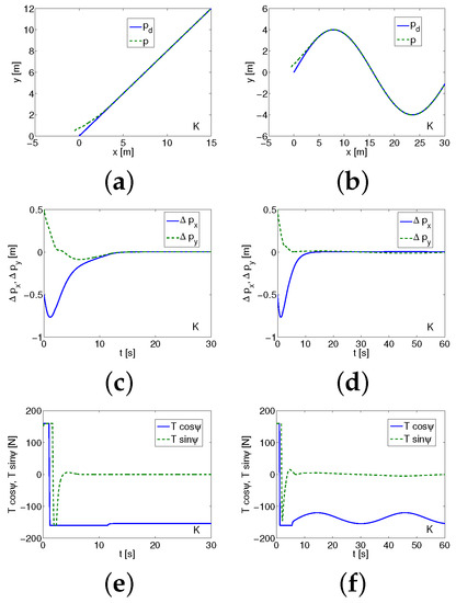
Figure 2.
Simulation results for Kambara (Lyapunov method-based controller (MBC))—linear and sine trajectory. (a,b) Desired and realized trajectory; (c,d) position errors; (e,f) applied forces/torques.
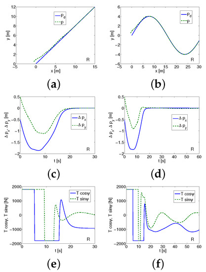
Figure 3.
Simulation results for ROPOS (Lyapunov MBC)—linear and sine trajectory. (a,b) Desired and realized trajectory; (c,d) position errors; (e,f) applied forces/torques.
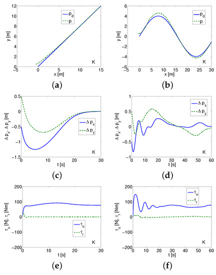
Figure 4.
Simulation results for Kambara (SMC/backstepping)—linear and sine trajectory. (a,b) Desired and realized trajectory; (c,d) position errors; (e,f) applied forces/torques.
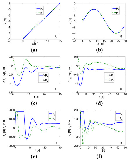
Figure 5.
Simulation results for ROPOS (SMC/backstepping)—linear and sine trajectory. (a,b) Desired and realized trajectory; (c,d) position errors; (e,f) applied forces/torques.
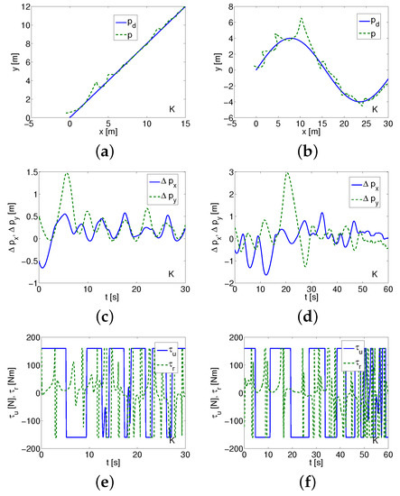
Figure 6.
Simulation results for Kambara (SMC)—linear and sine trajectory. (a,b) Desired and realized trajectory; (c,d) position errors; (e,f) applied forces/torques.
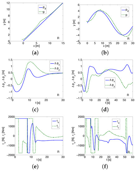
Figure 7.
Simulation results for ROPOS (sliding mode controller (SMC))—linear and sine trajectory. (a,b) Desired and realized trajectory; (c,d) position errors; (e,f) applied forces/torques.
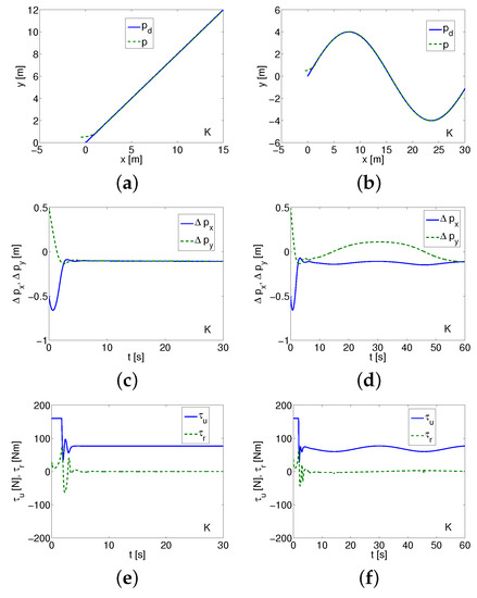
Figure 8.
Simulation results for Kambara (terminal sliding mode control (TSMC))—linear and sine trajectory. (a,b) Desired and realized trajectory; (c,d) position errors; (e,f) applied forces/torques.
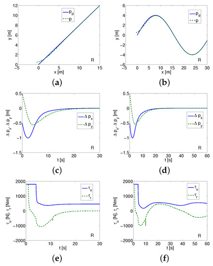
Figure 9.
Simulation results for ROPOS (TSMC)—linear and sine trajectory. (a,b) Desired and realized trajectory; (c,d) position errors; (e,f) applied forces/torques.
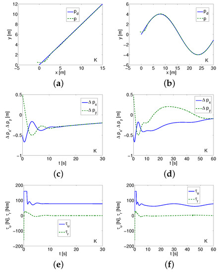
Figure 10.
Simulation results for Kambara (fast TSMC (FTSMC))—linear and sine trajectory. (a,b) Desired and realized trajectory; (c,d) position errors; (e,f) applied forces/torques.
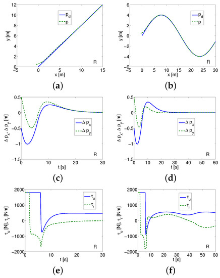
Figure 11.
Simulation results for ROPOS (FTSMC)—linear and sine trajectory. (a,b) Desired and realized trajectory; (c,d) position errors; (e,f) applied forces/torques.
For Lyapunov MBC (linear trajectory), the following values of the parameters were assumed: m (Kambara) and m (ROPOS) m, . Originally, the algorithm was appropriate for a hovercraft, therefore, two underwater vehicles are tested then averaged inertial parameters have been used, i.e., kg, kgm (Kambara) and kg, kgm (ROPOS). The controller gains were (K-Kambara, R-ROPOS):
The parameters estimated during simulations were off.
From Figure 2a, one can see that for Kambara the controller works correctly. This is confirmed in Figure 2c where both position errors tend to constant values close to zero (note that is assumed arbitrarily). From Figure 2e, it is observed that the forces have maximal or almost maximal values while the vehicle is in motion. Comparing the above results with the results obtained from ROPOS (Figure 3), it can be noticed that the tracking task is realized after a longer time than before (after about 20 s) as it is given in Figure 3a,c and the applied forces have maximal values for a very long time (Figure 3e).
Lyapunov MBC (sine trajectory). The same conditions of simulations, as for the linear trajectory tracking, were assumed. However, the applied control gains were different, namely:
As shown in Figure 2b,d, the trajectory tracking task is realized for Kambara although some non-zero errors on the y axis are visible. The applied forces change during the motion of the vehicle (Figure 2f) but they have acceptable even very high values. For ROPOS, a satisfactory trajectory tracking result can be obtained as it is visible in Figure 3b,d. The position errors are bigger than for Kambara and they are greater after the vehicle starts. However, the applied forces change when the vehicle is moving as can be seen in Figure 3f.
It turned out that for SMC/backstepping (linear trajectory), the selection of control coefficients is very difficult due to the sensitivity of the parameters. After many unsuccessful attempts, it was decided to choose the following set of control gains:
From Figure 4a,c, it is noticeable that the algorithm is effective for Kambara although with significant position errors. The steady state is obtained after about 28 s. The force and the torque are not very great as is presented in Figure 4e.
For ROPOS, much worse results were obtained for position errors, as shown in Figure 5a,c. The applied force and torque values are still acceptable (Figure 5e) despite the fact that in the first phase of movement they have maximal limit values. However, it is difficult to deduce whether for the assumed operating conditions the controller is effective.
SMC/backstepping (sine trajectory). It was noticed that similar problems arise as in the selection of gains for the linear trajectory. Finally, the following control gains set was assumed:
As can be seen from Figure 4b,d, tracking the sine trajectory for Kambara vehicle is inefficient despite the convergence of position errors because the errors are not close to zero. Maximum applied force and torque have acceptable values as shown in Figure 4f.
Comparing the obtained results for ROPOS, from Figure 5b,d, it is noticeable that the tracking task is also not realized correctly due to significant position error values. The force and torque change all the time during movement as it is observed in Figure 5f.
For SMC (linear trajectory), it was impossible to obtain satisfactory results of the tracking trajectory. The controller’s work is highly sensitive to parameter changes and depends on the integration method. After a long search for the right set of parameters, the following set of parameters was chosen:
As shown in Figure 6a,c for Kambara, the control task is not realized because of great position errors and velocities oscillations. Moreover, because of the force and the torque changes (Figure 6e), the vehicle would be destroyed.
For ROPOS, the tracking task is also not realized as it arises from Figure 7a,c,e.
SMC (sine trajectory). Additionally in this case, problems such as for linear trajectory were encountered. After many attempts, the selected parameters set was as follows:
Figure 6a,d illustrate that for Kambara, realization of the tracking control task is ineffective. Figure 6f shows values of the force and the torque. The simulation results indicate that changing these values will destroy the vehicle and the task will not be completed anyway.
The results obtained for ROPOS were also bad and unacceptable. The position error values were great (Figure 7b,d) and changes of the force and the torque may also damage the vehicle as it arises from Figure 7f.
The selection of gains for TSMC (linear trajectory) was easier. It was decided to assume the following parameters:
For Kambara, as it results from Figure 8a,c, the control algorithm works quickly (in about 4 s the steady-state is achieved but it is not zero, namely −0.1 m). The position error values are small (which is evident from Figure 8c), the force and the torque (given in Figure 8e) reach their final value in a short time.
For ROPOS, reaching the steady state requires longer time as it can be seen in Figure 9a,c. Values of the position errors are close to zero after about 25 s. However, this may be due to the fact that this vehicle is much heavier than Kambara. The force and the torque values (Figure 9e) are acceptable so that the controller works well.
TSMC (sine trajectory). For Kambara, the assumed set of parameters was , , , (and the others were as for the linear trajectory). Similarly, for ROPOS the set of parameters was , (and the others were as for the linear trajectory). Figure 8b,d show that tracking the sine trajectory for Kambara is possible but inaccurate due to the obtained end position error values. As can be seen from Figure 8f, in the initial phase of movement the force and the torque increase significantly but then decrease. However, their values are acceptable.
Better effects of control can be obtained for ROPOS. The desired trajectory is tracked correctly (Figure 9b) and the steady state of the position errors is obtained after about 20 s what is presented in Figure 9d. The applied force and torque have acceptable values as illustrated Figure 9f.
The difficulty of selecting parameters for FTSMC (linear trajectory) was similar to that of TSMC. Finally, it was assumed the set of parameters as follows:
For tests of TSMC and FTSMC, the values and were applied.
As can be seen in Figure 10a,c, for Kambara, the position error values are not close to zero but to a certain value (about m). Therefore, trajectory tracking may be considered not accurate enough. The force and the torque shown in Figure 10e have acceptable values. For ROPOS, the controller works correctly as seen from Figure 11a,c and the steady state is achieved. The signals, representing the applied force and the torque, given in Figure 11e indicate that the controller has performed the task correctly. FTSMC (sine trajectory). Similarly to the linear trajectory, the same values of gains for vehicles Kambara and ROPOS were used here. As shown in Figure 10b,d, for Kambara, the trajectory is not tracked accurately despite the fact that the position error values tend to some end value but not close to zero (about m). The force and torque given in Figure 10f are similar as for TSMC but without oscillation effect if the vehicle starts. For ROPOS, as it results from Figure 11b,d, the tracking task is realized correctly but after a slightly longer period of time than for TSMC (after about 30 s the steady state is achieved). The applied force and the torque, shown in Figure 11f have acceptable values.
Discussion of Results
Summarizing the obtained simulation results, the following observation can be made and conclusions can be drawn.
Comment on manual selection of gains. The method of manual selection of control parameters, i.e., the trial and error method, can be effective as long as the relationships between these parameters are noticeable (or one can recognize such groups of parameters for which there is such a relationship) that regulate the same physical quantity, e.g., reaching a sliding surface, ensuring the position, and velocity errors convergence. One can set a few parameters and then tune others and possibly change the previous values. This is some sort of heuristic method, but sometimes it turns out to be effective. In such cases, manual selection of parameters is possible even if there are many of them. This type of observation was used, for example, in work [47] where 24 control parameters were selected. The relationship between the control parameters can also be detected using a genetic algorithm, as noted in the paper [48] (for 18 control parameters). Unfortunately, for the control algorithms that did not lead to the achievement of acceptable results, it was not possible to find relations facilitating effective control. Perhaps the application of an additional method, e.g., a genetic algorithm, method of parameter optimization, would lead to an improvement in the results. However, doing so does not fall within the scope of the proposed test.
For Lyapunov MBC, the gains were tuned using the trial and error method based on the taken from [4]. For SMC/backstepping, the values of parameters , were determined (these gains can be grouped), and then attempts were made to tune the remaining gains (by trial and error method recommended in [11]). For the SMC method described in [17], some relationships between , , , and were noted and parameters were tuned on this basis. However, it turned out that the impact of other parameters is so important that the method previously indicated could not guarantee the convergence of errors. For the control TSMC strategy given [18] after initial determination of values , , , and , it is possible to look for the value of the proportion , (manual selection of parameters) so as to guarantee the convergence of errors in the assumed time (here s or s). Next, , and , should be chosen. Then it is necessary to tune the values of the preselected parameters , , , and . In addition, for FTSMC, the smallest possible values for and must be selected to avoid loss of stability.
In order to compare the algorithms in terms of ensuring the convergence of tracking errors, the mean values and standard deviations were calculated for each controller, for each trajectory and for both vehicles. The results are shown in Table 2.
Table 2.
Means (m) and standard deviations (std) of tracking errors.
Effectiveness of the tested control algorithms based on simulation results is presented in Table 3. It was also noted that for the algorithms that turned out to be effective, it is possible to slightly change the parameters to obtain acceptable control results.
Table 3.
Effectiveness of controllers based on simulations.
Despite the satisfactory results obtained in all tested cases, the Lyapunov MBC has significant drawbacks from a practical point of view. Due to the intended use of for a hovercraft, the mass in the longitudinal and transverse directions must be the same, which requires averaging and thus distorts the vehicle model. The vehicle must be equipped with a rudder and the tested vehicles have a different propulsion. Even if the structure of the vehicle could be changed, the tests show that the forces in motion have maximum permissible values or very large values. It is not known, therefore, whether such steering would be possible with a rudder. However, an undoubted advantage of the algorithm is an insight into the dynamics of the vehicle even with a completely different design. The algorithm can be used to check the effectiveness of underwater vehicle control and to determine the forces necessary to implement tracking of a desired trajectory. Such results are shown in Figure 2 (Kambara) and in Figure 3 (ROPOS) for linear and sine trajectory, respectively.
Effectiveness of SMC/backstepping has not been clearly confirmed. Satisfactory results, for linear trajectory, for Kambara were achieved, while worse for ROPOS (Figure 5). Unfortunately, for the sine trajectory, the tracking task is not carried out for any of the two tested vehicle models as it is presented in Figure 4 and Figure 5. Certainly, SMC/backstepping requires more thorough testing, but current tests show that the effectiveness of this algorithm depends significantly on the task and the conditions of its implementation (e.g., shape of the trajectory, vehicle dynamics).
For SMC, no acceptable results were obtained for Kambara and ROPOS, neither for linear trajectory nor sine trajectory as it is seen in Figure 6 and Figure 7. It is difficult to say in what conditions this algorithm can be used because the only case of its correct operation was obtained for the vehicle and conditions indicated in work [17].
With the use of TSMC for Kambara (Figure 8), convergence of the position errors was very quickly achieved, but only up to a certain non-zero value (about −0.1 m) for linear trajectory. The results show that the controller does not guarantee convergence of these errors to zero. Other values of variables indicate the algorithm works effectively. For the sine trajectory tracking task (Figure 8) also some position error values occur which are not close to zero. TSMC effectiveness was confirmed for ROPOS and linear trajectory by convergence the position errors to zero with acceptable time history of other physical quantities (Figure 9). If the sine trajectory is tracked then the control algorithm gives also satisfactory results.
Simulation results obtained for FTSMC, linear trajectory and Kambara vehicle show that the position errors only go to a limited value other than zero (Figure 10). At the same time, the applied force and torque have acceptable values which indicate that the algorithm is working properly. Similar results were obtained for the sine desired trajectory as it is given in Figure 10. For ROPOS, the tracking errors tend to zero for both linear and sine trajectories at acceptable values of other tested variables (Figure 11). Satisfactory results can also be obtained for sine trajectory as shown also in Figure 11.
Comment on the results from Table 2 and Table 3. Acceptable results by both tables were obtained for Kambara and both trajectories (Lyapunov MBC), for ROPOS and sine trajectory (TSMC), as well as for ROPOS and both trajectories (FTSMC). Table 2 shows that acceptable results were obtained for SMC/backstepping (sine) and TSMC (sine) for the Kambara. However, it can be seen from Figure 4d and Figure 8d that the trajectory tracking task is not being performed correctly. On the other hand, from Figure 3c,d, it can be noticed that for the ROPOS vehicle (linear and sine trajectory), the use of the Lyapunov MBC algorithm is effective, although the mean and standard deviation values do not indicate it. A similar observation can be made by comparing Figure 9c for ROPOS (linear trajectory) and the TSMC algorithm with the values of standard deviation and mean. It can therefore be concluded that to evaluate the work of the controller, both objective criteria (here: std and mean) and subjective criteria, i.e., the evaluation of tracking errors based on figures obtained in simulations, are necessary.
Based on the tests performed, it can be concluded that the trajectory tracking results for TSMC and FTSMC depend on the underwater vehicle being tested. TSMC and FTSMC proved in simulations to be the most promising. SMC/backstepping is also worth more detailed research. To sum up, however, to show the real effectiveness of the control algorithms, more detailed tests would be required to determine the scope of applicability of these algorithms. It can be supposed that unsatisfactory results are due to inadequate choice of parameters. However, no rules for the correct selection of control parameters were found in the reference works. Research has shown that obtaining satisfactory control results is difficult and in some cases not possible. Therefore, if the selection of parameters by means of an intuitive method is really difficult for a control algorithm, then in the source works additional methods should be given to facilitate this task, as in [48,49].
Additional test for effective algorithms were performed for selected control algorithms with taking into consideration disturbances functions.
For SMC/backstepping, Kambara, and linear trajectory the time-varying disturbances were assumed as in [11], namely: N and Nm. For TSMC, FTSMC ROPOS and linear and also sine trajectory, the time-varying disturbances of the type as in [18] were applied: N, N.
However, the control parameters had to be changed to obtain satisfactory control performance. The following control gains set was chosen for Kambara and C2:
For ROPOS and C4 (linear trajectory), the following set of parameters was used:
For ROPOS C4 (sine trajectory), the following set of parameters was used:
For ROPOS C5 (sine trajectory), the following set of parameters was used:
As it can be observed from Figure 12 and Figure 13, all controllers work correctly. For SMC/backstepping (Kambara), the results are only slightly different (cf. Figure 4). However, the algorithm reaches the steady state after a long time. For TSMC (ROPOS) and linear trajectory, the position errors are smaller than previously (cf. Figure 9) but the applied forces/torques time history is different. For TSMC and FTSMC (ROPOS) and sine trajectory, a similar observations can be made (cf. Figure 9 and Figure 10). For FTSMC, the position errors are bigger in the second phase of motion and next the trajectory is traced correctly. From the conducted test, it can be concluded that if the algorithms work properly in the initial test, they also work with disturbances of the type as in the source literature.
Figure 12.
Simulation results for SMC/backstepping Kambara (K) and TSMC ROPOS (R)—linear trajectory. (a,b) Desired and realized trajectory; (c,d) position errors; (e,f) applied forces/torques.
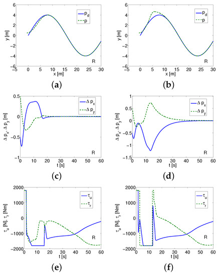
Figure 13.
Simulation results for sine trajectory and ROPOS TSMC—left, and FTSMC—right. (a,b) Desired and realized trajectory; (c,d) position errors; (e,f) applied forces/torques.
5. Conclusions
Selected algorithms for tracking the trajectory of underwater vehicles moving horizontally with insufficient force input were tested in the work. Five control algorithms were compared in terms of their suitability on two exemplary vehicle models. The first control scheme originally dedicated to hovercraft is primarily used to learn about the behavior of the vehicle when it is necessary to follow a desired trajectory.
The obtained simulation results for two models of 3-DOF vehicles, i.e., Kambara and ROPOS, provided information on the suitability of each algorithm under the assumed operating conditions and for two different trajectories. Based on the graphs of tracking errors as well as and on graphs of other physical quantities (treated as subjective evaluation measures), and the values of means and standard deviations (treated as objective evaluation measures), the obtained results were discussed. It turned out that the selected methods of tracking the trajectory of underwater vehicles may not guarantee the satisfactory results that were obtained in the original works. However, due to the fact that only the results of preliminary tests of control algorithms are presented, the possibility of introducing additional methods of searching for the controller parameters (e.g., based on optimization techniques, genetic algorithms) should be considered in the future. In this study, such a possibility was not assumed, because its aim was to apply a simple method of searching for these parameters under the assumed operating conditions. The proposed approach can be used as a preliminary test before experimental research to compare selected models of systems or to decide whether the selected algorithm is worth the risk if it is used in a real experiment. Based on the simulations, it was found that even if the algorithm worked correctly in the original source, it may not be effective in the case of changed vehicle models or working conditions. It follows that having a model of a vehicle, it is necessary to check the effectiveness of the algorithm selected from the literature. In the future, more detailed simulation tests of selected control strategies should be carried out to determine their potential usefulness in experimental research based on simulations. It may turn out that an expensive experiment will not confirm the effectiveness of the selected algorithms, and this could be avoided by conducting a simulation test earlier. Moreover, since disturbances are considered only in some cases in the presented work, this issue should also be considered in further research.
Funding
The work was supported by Poznan University of Technology Grant No. 09/93/DSPB/0611.
Conflicts of Interest
The author declares no potential conflicts of interest with respect to the research, authorship, and/or publication of this article.
References
- Behal, A.; Dawson, D.M.; Dixon, W.E.; Fang, Y. Tracking and Regulation Control of an Underactuated Surface Vessel with Nonintegrable Dynamics. IEEE Trans. Autom. Control 2002, 47, 495–500. [Google Scholar]
- Do, K.D.; Jiang, Z.P.; Pan, J. Underactuated Ship Global Tracking Under Relaxed Conditions. IEEE Trans. Autom. Control 2002, 47, 1529–1536. [Google Scholar]
- Pettersen, K.Y.; Nijmeijer, H. Underactuated ship tracking control: Theory and experiments. Int. J. Control 2001, 74, 1435–1446. [Google Scholar]
- Cabecinhas, D.; Batista, P.; Oliveira, P.; Silvestre, C. Hovercraft Control with Dynamic Parameters Identification. IEEE Trans. Control Syst. Technol. 2018, 26, 785–796. [Google Scholar]
- Ferreira, C.Z.; Cardoso, R.; Meza, M.E.M.; Avila, J.P.J. Controlling tracking trajectory of a robotic vehicle for inspection of underwater structures. Ocean Eng. 2018, 149, 373–392. [Google Scholar]
- Repoulias, F.; Papadopoulos, E. Planar trajectory planning and tracking control design for underactuated AUVs. Ocean Eng. 2007, 34, 1650–1667. [Google Scholar]
- Zhang, Z.; Wu, Y. Further results on global stabilisation and tracking control for underactuated surface vessels with non-diagonal inertia and damping matrices. Int. J. Control 2015, 88, 1679–1692. [Google Scholar]
- Zhou, J.; Ye, D.; Zhao, J.; He, D. Three-dimensional trajectory tracking for underactuated AUVs with bio-inspired velocity regulation. Int. J. Nav. Archit. Ocean Eng. 2018, 10, 282–293. [Google Scholar]
- Do, K.D. Robust adaptive tracking control of underactuated ODINs under stochastic sea loads. Robot. Auton. Syst. 2015, 72, 152–163. [Google Scholar]
- Aguiar, A.P.; Hespanha, J.P. Trajectory-Tracking and Path-Following of Underactuated Autonomous Vehicles With Parametric Modeling Uncertainty. IEEE Trans. Autom. Control 2007, 52, 1362–1379. [Google Scholar]
- Xu, J.; Wang, M.; Qiao, L. Dynamical sliding mode control for the trajectory tracking of underactuated unmanned underwater vehicles. Ocean Eng. 2015, 105, 54–63. [Google Scholar]
- Pettersen, K.Y.; Nijmeijer, H. Global practical stabilization and tracking for an underactuated ship–A combined averaging and backstepping approach. Model. Identif. Control 1999, 20, 189–199. [Google Scholar]
- Yu, H.; Guo, C.; Shen, Z.; Yan, Z. Output Feedback Spatial Trajectory Tracking Control of Underactuated Unmanned Undersea Vehicles. IEEE Access 2020, 8, 42924–42936. [Google Scholar]
- Li, S.; Wang, X.; Zhang, L. Finite-Time Output Feedback Tracking Control for Autonomous Underwater Vehicles. IEEE J. Ocean. Eng. 2015, 40, 727–751. [Google Scholar]
- Nijmeijer, H. A global output-feedback controller for stabilization and tracking of underactuated ODIN: A spherical underwater vehicle. Automatica 2004, 40, 117–124. [Google Scholar]
- Ashrafiuon, H.; Nersesov, S.; Clayton, G. Trajectory Tracking Control of Planar Underactuated Vehicles. IEEE Trans. Autom. Control 2017, 62, 1959–1965. [Google Scholar]
- Elmokadem, T.; Zribi, M.; Youcef-Toumi, K. Trajectory tracking sliding mode control of underactuated AUVs. Nonlinear Dyn. 2016, 84, 1079–1091. [Google Scholar]
- Elmokadem, T.; Zribi, M.; Youcef-Toumi, K. Terminal sliding mode control for the trajectory tracking of underactuated Autonomous Underwater Vehicles. Ocean Eng. 2017, 129, 613–625. [Google Scholar]
- Yan, Z.; Yu, H.; Zhang, W.; Li, B.; Zhou, J. Globally finite-time stable tracking control of underactuated UUVs. Ocean Eng. 2015, 107, 132–146. [Google Scholar]
- Zhou, J.; Zhao, X.; Chen, T.; Yan, Z.; Yang, Z. Trajectory Tracking Control of an Underactuated AUV Based on Backstepping Sliding Mode with State Prediction. IEEE Access 2019, 7, 181983–181993. [Google Scholar]
- Chen, L.; Cui, R.; Yang, C.; Yan, W. Adaptive Neural Network Control of Underactuated Surface Vessels with Guaranteed Transient Performance: Theory and Experimental Results. IEEE Trans. Ind. Electron. 2020, 67, 4024–4035. [Google Scholar]
- Park, B.S. Neural Network-Based Tracking Control of Underactuated Autonomous Underwater Vehicles With Model Uncertainties. J. Dyn. Syst. Meas. Control. Trans. ASME 2015, 137, 021004. [Google Scholar]
- Yan, Z.; Wang, M.; Xu, J. Robust adaptive sliding mode control of underactuated autonomous underwater vehicles with uncertain dynamics. Ocean Eng. 2019, 173, 802–809. [Google Scholar]
- Zhang, C.; Wang, C.; Wei, Y.; Wang, J. Neural-Based Command Filtered Backstepping Control for Trajectory Tracking of Underactuated Autonomous Surface Vehicles. IEEE Access 2020, 8, 42482–42490. [Google Scholar]
- Mu, D.; Wang, G.; Fan, Y.; Qiu, B.; Sun, X. Adaptive Trajectory Tracking Control for Underactuated Unmanned Surface Vehicle Subject to Unknown Dynamics and Time-Varing Disturbances. Appl. Sci. 2018, 8, 547. [Google Scholar]
- Chen, Y.; Ruan, L.; Ming, Z. Adaptive fuzzy inverse trajectory tracking control of underactuated underwater vehicle with uncertainties. Ocean Eng. 2016, 121, 123–133. [Google Scholar]
- Yu, C.; Xiang, X.; Zhang, Q.; Xu, G. Adaptive Fuzzy Trajectory Tracking Control of an Under-Actuated Autonomous Underwater Vehicle Subject to Actuator Saturation. Int. J. Fuzzy Syst. 2018, 20, 269–279. [Google Scholar]
- Xiang, X.; Yu, C.; Lapierre, L.; Zhang, J.; Zhang, Q. Survey on Fuzzy-Logic-Based Guidance and Control of Marine Surface Vehicles and Underwater Vehicles. Int. J. Fuzzy Syst. 2018, 20, 572–586. [Google Scholar]
- Sands, T. Development of Deterministic Artificial Intelligence for Unmanned Underwater Vehicles (UUV). J. Mar. Sci. Eng. 2020, 8, 578. [Google Scholar]
- Bechlioulis, C.P.; Karras, G.C.; Heshmati-Alamdari, S.; Kyriakopoulos, K.J. Trajectory Tracking With Prescribed Performance for Underactuated Underwater Vehicles Under Model Uncertainties and External Disturbances. IEEE Trans. Control. Syst. Technol. 2017, 25, 429–440. [Google Scholar]
- Li, J.; Du, J.; Sun, Y.; Lewis, F.L. Robust adaptive trajectory tracking control of underactuated autonomous underwater vehicles with prescribed performance. Int. J. Robust Nonlinear Control 2019, 29, 4629–4643. [Google Scholar]
- Guerreiro, B.J.; Silvestre, C.; Cunha, R.; Pascoal, A. Trajectory Tracking Nonlinear Model Predictive Control for Autonomous Surface Craft. IEEE Trans. Control. Syst. Technol. 2014, 22, 2160–2175. [Google Scholar]
- Heshmati-Alamdari, S.; Nikou, A.; Dimarogonas, D.V. Robust Trajectory Tracking Control for Underactuated Autonomous Underwater Vehicles in Uncertain Environments. IEEE Trans. Autom. Sci. Eng. 2020. [Google Scholar] [CrossRef]
- Paliotta, C.; Lefeber, E.; Pettersen, K.Y.; Pinto, J.; Costa, M.; de Figueiredo Borges de Sousa, J.T. Trajectory Tracking and Path Following for Underactuated Marine Vehicles. IEEE Trans. Control. Syst. Technol. 2019, 27, 1423–1437. [Google Scholar]
- Serrano, M.E.; Scaglia, G.J.E.; Godoy, S.A.; Mut, V.; Ortiz, O.A. Trajectory Tracking of Underactuated Surface Vessels: A Linear Algebra Approach. IEEE Trans. Control. Syst. Technol. 2014, 22, 1103–1111. [Google Scholar]
- Ye, L.; Zong, Q. Tracking control of an underactuated ship by modified dynamic inversion. ISA Trans. 2018, 83, 100–106. [Google Scholar]
- Antonelli, G. On the Use of Adaptive/Integral Actions for Six-Degrees-of-Freedom Control of Autonomous Underwater Vehicles. IEEE J. Ocean. Eng. 2007, 32, 300–312. [Google Scholar]
- Soylu, S.; Buckham, B.J.; Podhorodeski, R.P. A chattering-free sliding-mode controller for underwater vehicles with fault-tolerant infinity-norm thrust allocation. Ocean Eng. 2008, 35, 1647–1659. [Google Scholar]
- Silpa-Anan, C. Autonomous Underwater Robot: Vision and Control. Master’s Thesis, The Australian National University, Canberra, Australia, 2001. [Google Scholar]
- Xie, T.; Li, Y.; Jiang, Y.; An, L.; Wu, H. Backstepping active disturbance rejection control for trajectory tracking of underactuated autonomous underwater vehicles with position error constraint. Int. J. Adv. Robot. Syst. 2020, 17, 1–12. [Google Scholar] [CrossRef]
- Peng, Z.; Wang, J.; Han, Q.L. Path-Following Control of Autonomous Underwater Vehicles Subject to Velocity and Input Constraints via Neurodynamic Optimization. IEEE Trans. Ind. Electron. 2019, 66, 8724–8732. [Google Scholar]
- Yang, H.; Deng, F.; He, Y.; Jiao, D.; Han, Z. Robust nonlinear model predictive control for reference tracking of dynamic positioning ships based on nonlinear disturbance observer. Ocean Eng. 2020, 215, 107885. [Google Scholar]
- Kicki, P.; Kozlowski, J. Software for “Hovercraft Control With Dynamic Parameters Identification”; Poznan University of Technology: Poznań, Poland, 2018; Unpublished project. [Google Scholar]
- Grabarczyk, E. Implementation of Selected Control Algorithms for an Underactuated Marine Vehicle Model. Master’s Thesis, Poznan University of Technology, Poznań, Poland, 2018. [Google Scholar]
- Szczech, A.; Wawrzenczak, J. Software for “Trajectory tracking sliding mode control of underactuated AUVs”; Poznan University of Technology: Poznań, Poland, 2018; Unpublished project. [Google Scholar]
- Gryczka, N.; Rychlewicz, K. Software for “Terminal Sliding Mode Control for the Trajectory Tracking of Underactuated Autonomous Underwater Vehicles”; Poznan University of Technology: Poznań, Poland, 2018; Unpublished project. [Google Scholar]
- Herman, P. Application of nonlinear controller for dynamics evaluation of underwater vehicles. Ocean Eng. 2019, 179, 59–66. [Google Scholar]
- Herman, P.; Adamski, W. Nonlinear trajectory tracking controller for a class of robotic vehicles. J. Frankl. Inst. 2017, 354, 5145–5161. [Google Scholar]
- Lefeber, E.; Pettersen, K.Y.; Nijmeijer, H. Tracking Control of an Underactuated Ship. IEEE Trans. Control. Syst. Technol. 2003, 11, 52–61. [Google Scholar]


Publisher’s Note: MDPI stays neutral with regard to jurisdictional claims in published maps and institutional affiliations. |
© 2020 by the author. Licensee MDPI, Basel, Switzerland. This article is an open access article distributed under the terms and conditions of the Creative Commons Attribution (CC BY) license (http://creativecommons.org/licenses/by/4.0/).