Article

Two-Lane Highways Crest Curve Design. The Case Study of Italian Guidelines

DICAM-Department of Civil, Environmental and Mechanical Engineering, University of Trento, 38122 Trento, Italy
Appl. Sci. 2020, 10(22), 8182; https://doi.org/10.3390/app10228182
Submission received: 31 October 2020 / Revised: 15 November 2020 / Accepted: 16 November 2020 / Published: 18 November 2020
(This article belongs to the Special Issue Human Factors in Transportation Systems)

Abstract

:
The main purpose of the research is to evaluate the crest vertical curves radii Rv, not considering a conventional value of the opposing vehicle height h2, but the average vehicle heights h2(m) and the value of the 15th percentile of the height distribution h2(15) of the passenger car population. The study only considered car models with more than 20,000 registered vehicles in Italy. One hundred and fifteen car models belonging to different brands were taken into consideration, for a total of over 9 million vehicles. For the statistical sample analyzed, the following vehicle heights were estimated: h2(m) = 1.48 m and h2(15) = 1.39 m. The deviations between the crest radii calculated with the Italian standard (h2 = 1.10 m), and those obtained for h2(m) = 1.48 m and h2(15) = 1.39 m are up to 12%. The differences ΔHv between the values of the visible vehicle body height Hv = Hv(t) calculated using, respectively, h2(15) = 1.39 m and h2(m) = 1.48 m are modest. The value h2(m) = 1.48 m could be adopted in order to reduce the highways construction costs. In fact, the research shows that the value h2 = 1.10 m is too conservative and leads to oversizing of the crest vertical curves. Therefore, it would be necessary to make an appropriate choice of h2 value in order to take into account the current heights of passenger cars.

1. Introduction

In highway design, vertical curves have to be used to transition grade changes. Vertical curves should be chosen considering many relevant issues such as driver safety, comfort, alignment aesthetics, and drainage purposes [1,2,3,4]. Vertical curves are of two classes: convex vertical curves, known as crest curves, and concave vertical curves, known as sag curves [5,6]. Parabolic or circular curves are the common choices for vertical curves both in highway engineering [1,5,6] and in railway engineering [7,8]. Generally, parabolic curves are preferred, because they provide a constant rate of curvature change [6,9].
The main purpose of a crest curve’s design is to calculate the minimum vertical curve radius (Rv,min) that complies the required sight distance (stopping sight distance SSD or passing sight distance PSD), according to total grade change Δi, design speed v, and drivers’ comfort. As it is well known, too short a vertical curve radius may lead to insufficient sight distance.
Safe operation on crest vertical curves mainly depends on ample sight distance. Minimum stopping sight distance SSD should be ensured in all cases [6,9]. Table 1 shows the minimum radii of crest vertical curves as a function of design speed in various countries [6]. Wherever economically and technically feasible, passing sight distance PSD should be provided on two-lane highways [6,9].
In this article, the relationship between crest vertical curve radius Rv, passing sight distance PSD, driver eye height h1, object (i.e., opposing vehicle) height h2, and the characteristics of vehicle was obtained, considering for h2 not a conventional value (i.e., h2 = 1.10 m in the case of the Italian guidelines [10,11]) but the real vehicle heights. This is because, in recent decades, there has been a generalized significant increase in the vehicles’ height. For example, the roof top height of modern sport utility vehicles (SUVs) is often more than 1.70 m. Therefore, in order to evaluate a reasonable value for h2 a statistical sampling of the height of vehicles circulating in Italy was carried out. In particular, the average vehicle heights h2(m) and the value of the 15th percentile of the height distribution h2(15) have been calculated.
A comparative analysis between the vertical convex curves radii recommended in the Italian Guidelines for the Design of Road Infrastructures (h2 = 1.10 m) [10] and the homologous values calculated with the analytical relationships proposed in this research (based on h2(m) and h2(15) parameters) was developed.
The results show that the h2 value prescribed by the Italian guidelines [10,11] (h2 = 1.10 m) is excessively precautionary, since it results in h2(m) = 1.48 m and h2(15) = 1.39 m, respectively. It follows the oversizing of the radius of vertical convex curves and their length, with consequent greater highways construction costs.

2. The Overtaking Maneuver and the Passing Sight Distance (PSD)

The overtaking maneuver is a key issue for two-lane highways, because it requires occupying the opposing lane, which represents a serious safety concern [6,9,12,13].
Accidents occurred due to overtaking maneuvers represent around 38% of the total accidents on Italian two-lane highways [14]. Accident severity associated to overtaking maneuvers is usually higher than in other maneuver types [12,13].
The overtaking maneuver’s frequency depends on various factors, including traffic volumes, users’ motivation, and their psychophysical state and highway alignment (vertical and horizontal) [15]. The traffic flow variable that considerably influences the propensity to do an overtake maneuver is the vehicular density k. In steady-state traffic condition [16,17,18], the density k can be estimated by knowing the flow rate q and the mean space speed vs, with the well-known fundamental relations of traffic flow: k = q/vs.
As q increases for a given vehicle, the probability of encountering slow vehicles increases [19]. In other words, users have high probability to encounter slower vehicles and often are forced to queue up first and then overtake where the available sight distance D is greater than the passing sight distance PSD [19]. Consequently, the performance analyses of two-lane highways—whose objective is to determine the level of service (LOS) for an existing or proposed facility—include a specific evaluation of the percent time-spent-following [20].
Then, a PSD adequate for users to pass slow vehicles should be provided at frequent intervals on two-lane highways. In order to guarantee acceptable LOS, several highway design guidelines require a minimum percentage of passing zones in each direction of travel (e.g., 20% in Italy [10]).
To ensure suitable safety conditions, overtaking is only allowed in the zones where available sight distance is higher than the required overtaking passing sight distance PSD [12,21]. PSD is defined as the distance required to complete an overtaking maneuver when an opposing vehicle is approaching in the opposing lane.
The PSD can be estimated by means of several overtaking models. In the Italian model [10] (Figure 1), the speed v of overtaking vehicle (A) is assumed to be uniform during the right and left lanes occupation time. The speed of the overtaken vehicle B is v − ∆v. Instead, the speed of the opposing vehicle C, in the opposing lane, is v.
The minimum passing sight distance PSD is the sum of four subintervals [22]: d1 = v·t1; d2 = v·t2; d3 = v·t3; d4 = v·(t1 + t2 + t3), in which:
v: design speed of the highway segment under analysis expressed in m/s;
t1 = 4 s: time for lane change (from the right lane to the opposing lane);
t2 = 2 s: overtaking time (at the end of this time interval the rear bumper of vehicle A and the front bumper of vehicle B are at the same road section);
t3 = 4 s: time for lane change (from the opposing lane to the right lane).
Therefore, the minimum passing sight distance PSD is:
PSD =   2 v   ( t 1 + t 2 + t 3 )   =    2 v   ( t 1 + 2 l m Δ v + t 3 )
where:
lm = (lA + lB)/2;
lA length of the vehicle A;
lB length of the vehicle B.
Since   l m Δ v 1   s , it results in:
PSD   =   20 v = 5.5   V   [ m ]
in which V is the design speed expressed in km/h.
Figure 2 illustrates a comparison of minimum PSD values obtained with the several widespread models of Table 2, including the Italian model, in function of the highway design speed V.

3. Analytical Derivation of Crest Curve Minimum Radius

The minimum radius of crest curves based on passing sight distance (PSD) criteria generally is satisfactory from the standpoint of safety, comfort, and appearance [15,22]. In this section, the detailed derivation process for the analytical relationship between passing sight distance (PSD), driver eye height h1, object (i.e., opposing vehicle) height h2, and the necessary parabolic vertical crest curve radius Rv is presented.
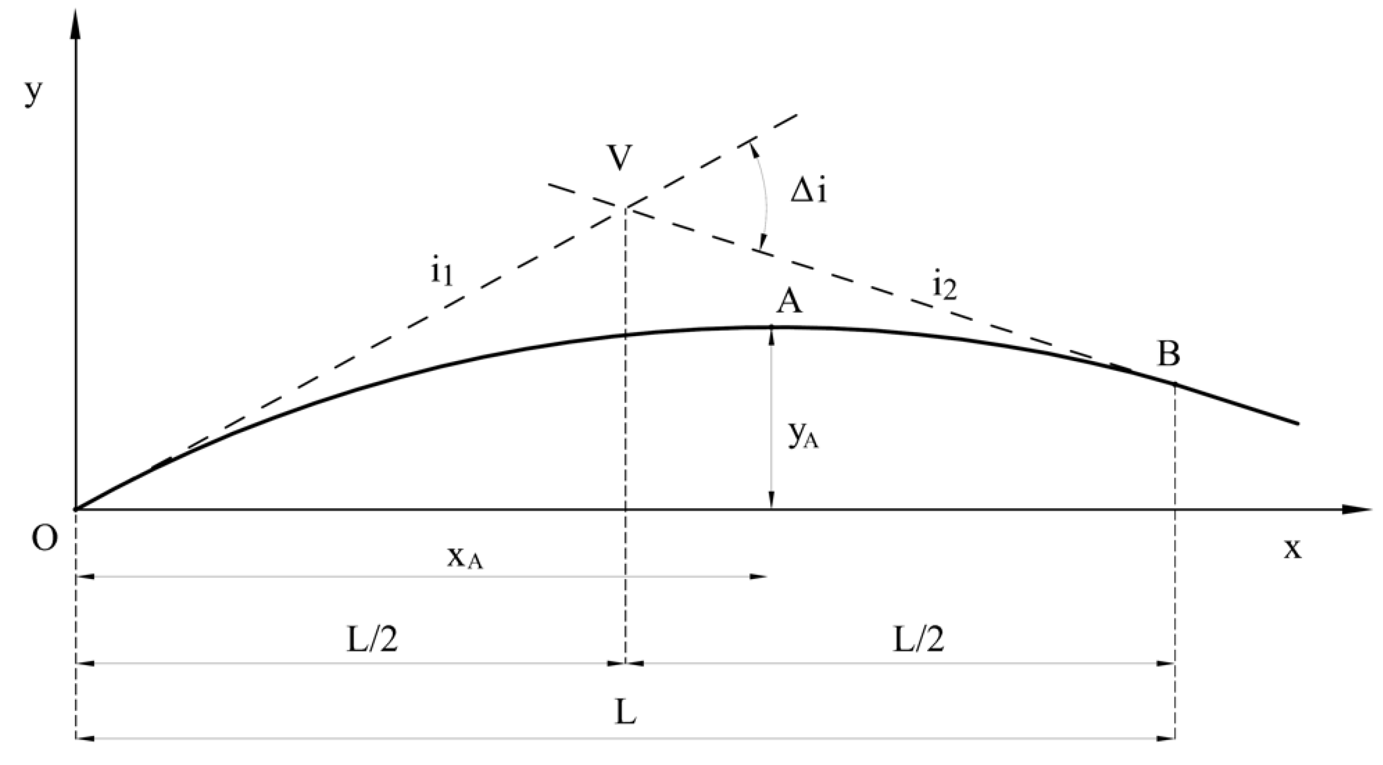
Let the left-hand side road grade be i1, and right-hand side road grade i2, the total grade change Δi = i2 − i1 < 0 (assuming i2 < i1), and L the crest vertical curve length. The origin of the coordinates is selected at point O (beginning of the vertical curve) (Figure 3). If the vertical curve follows a parabolic shape, the curve equation is:
y = ax2 + bx
The coefficients a and b can be obtained by the following boundary conditions:
( dy dx ) x = 0 = b     therefore     b = i 1
d 2 y dx 2 = 2 a     therefore     a = Δ i 2 L
The vertical curve equation y = ax2 + bx can be rewritten as Equation (6)
y = Δ i 2 L x 2 + i 1 x
the coordinates in the summit of the parabola (point A of Figure 3) are:
x A = i 1 Δ i L
y A = i 1 2 2 Δ i L
the relationship of the curvature is:
1 R = Δ i L [ 1 + ( Δ i L x + i 1 ) 2 ] 3 2
Equation (9) allows to calculate the radius of the osculating circle in the points O, A, and B:
R o = [ 1 + i 1 2 ] 3 2 Δ i L
R B = [ 1 + ( i 1 + Δ i ) 2 ] 3 2 Δ i L
R A = L Δ i  
The minimum radius of curvature Rv is located at point A, therefore we can assume Rv = RA. Let D = PSD (cfr. Figure 4). The relationship between the minimum radius of curvature Rv, the passing sight distance D, the driver eye height h1, object (i.e., opposing vehicle) height h2, and the total grade change Δi can be derived using the geometric schemes, as depicted in Figure 4. More specifically, Figure 4 illustrates the influence of vertical curvature on visibility. Two conditions must be considered [1,9,22,31]:
  • Passing sight distance is shorter than vertical curve length (D < L);
  • Passing sight distance is longer than vertical curve length (D > L).

3.1. Case in Which D < L

Consider the case in which the passing sight distance is shorter than the vertical curve length (D = PSD < L). Using the geometric parameters in Figure 4, it results in [22]:
h 1 = ap 2
h 2 = aq 2
D = p + q = 1 a · ( h 1 + h 2 )
L = Δ i · D 2 2 · ( h 1 + h 2 + 2 h 1 · h 2 )
R V = R A = L Δ i = D 2 2 · ( h 1 + h 2 + 2 h 1 · h 2 )
According to Equation (17), the minimum radius of curvature Rv (point A of Figure 3) is not a function of the total grade change Δi.

3.2. Case in Which D > L

Consider the case in which the passing sight distance is longer than the vertical curve length (D = PSD > L). Using the geometric parameters in Figure 4, it results in [22]:
h 1 = a · p 2 + 2 · a · p · m 1
h 2 = a · q 2 + 2 · a · q · m 2
m 1 = h 1 2 · a · p p 2
m 2 = h 2 2 · a · q q 2
D = m 1 + L + m 2 = h 1 2 · a · p + h 2 2 · a · ( L p ) + L 2
The minimum value of the sight distance can be obtained deriving the Equation (22) and by the following condition:
dD dp = h 1 2 · a · p 2 + h 2 2 · a · ( L p ) 2 = 0
then
p = L 1 + h 2 h 1
q = L p = p · h 2 h 1
plug Equations (24) and (25) into Equation (22), after minor rearrangement, it results in:
D = L 2 + h 1 + h 2 + 2 · h 1 · h 2 Δ i
L = 2 · ( D h 1 + h 2 + 2 · h 1 · h 2 Δ i )
R V = R A = 2 Δ i · ( D h 1 + h 2 + 2 · h 1 · h 2 Δ i )
According to Equation (28), the minimum radius of curvature Rv (point A of Figure 3) is a function of the total grade change Δi.

4. Passing Sight Distance, Opposing Vehicle Height h2, and Eye Height h1

An object (i.e., opposing vehicle) height of h2 = 1.10 m is adopted by the Italian Guidelines for the Design of Road Infrastructures [10] for the calculation of passing sight distance PSD. Such value appears not to be in compliance with the average height of the current passenger car population. In fact, over the past few decades, sales of sport utility vehicles (SUVs) have increased. At the same time, even utility cars have undergone increases in overall size and, in particular, in height.
For this reason, a specific analysis was carried out concerning the Italian passenger car population until 2006, coinciding with the year of publication of the latest Italian Guidelines for the Design of Road Intersections [11].
The research was carried out using the Italian car population data updated to 31 December 2006, registered by the Italian Automobile Club (ACI) and by the Public Vehicle Registration Office (PRA) [32]. On that date, the vehicles circulating in Italy were 35,297,282. The study only considered car models with more than 20,000 registered vehicles. Specifically, 115 vehicle models belonging to different brands were taken into consideration, for a total of over 9 million vehicles. For each of the 115 models considered, the overall height was deduced.
Table 3 shows the summary data. In the study, the average vehicle heights h2(m) and the value corresponding to the 15th percentile of the height distribution h2(15) were estimated, obtaining, respectively, the values h2(m) = 1.48 m and h2(15) = 1.39 m.
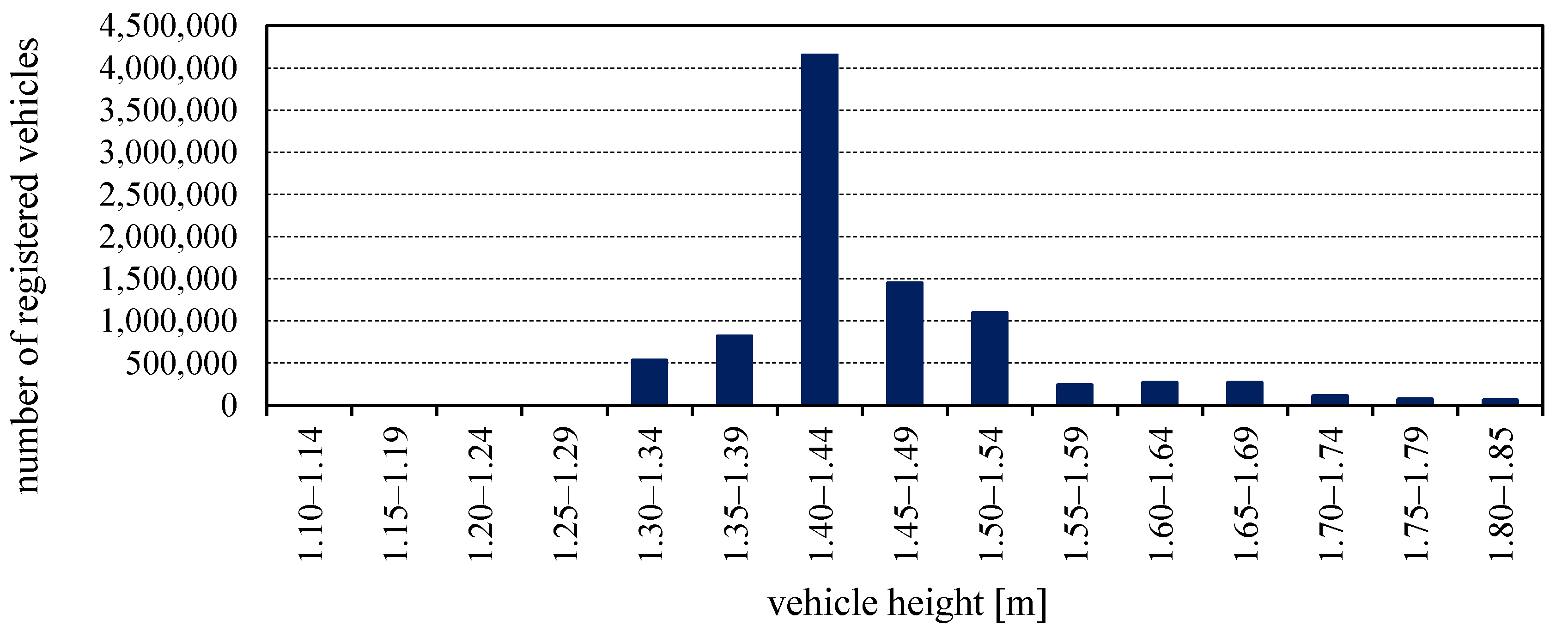
As shown in the histogram of Figure 5, the largest number of registered vehicles (4,151,428) falls in the height range 1.40–1.44 m, follow the intervals 1.45–1.49 m and 1.50–1.54 m, with 1,449,211 and 1,100,024 vehicles, respectively. The sum of the vehicles falling into these three classes is 6,700,663, namely the 73% of the number of passenger cars examined.
According to the Italian Guidelines for the Design of Road Infrastructures and Intersections [10,11], the obstacle that the driver must be able to see during the overtaking maneuver (i.e., opposing vehicle) has a height h2 = 1.10 m. Evidently, this is a very conservative value compared to the inferred values h2(m) = 1.48 m and h2(15) = 1.39 m. The remarkable differences between the height of the obstacle provided by the Italian guideline (h2) and those derived from the real passenger car population (h2(m) and h2(15)) lead to significant differences in the values of the radii of the crest curve (Rv). Instead, the driver’s eye height h1 = 1.10 m is congruent with the values adopted internationally (Table 4) [33].

Minimum Values of Rv

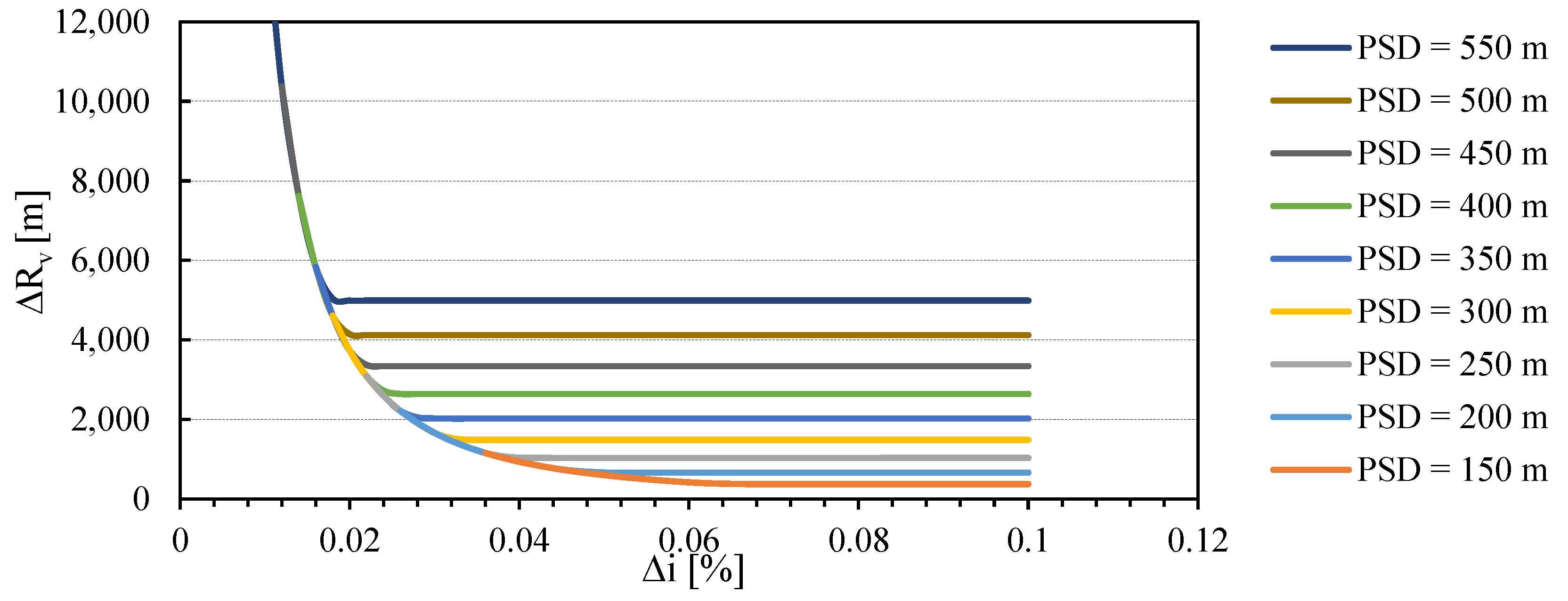
Figure 6 shows Rv values according to the Equations (17) and (28) obtained for h1 = 1.10 m and h2(15) = 1.39 m. Similarly, Figure 7 shows Rv values according to the Equations (17) and (28) obtained for h1 = 1.10 m and h2(m) = 1.48 m. In both cases, each curve Rv(∆i) reaches a maximum value Rv * for ∆i = ∆i *; instead, for ∆i > ∆i *, it results in Rv = Rv *. As can be observed from Figure 8, the differences ΔRv between Rv values calculated in the two scenarios (h2(15) = 1.39 m and h2(m) = 1.48 m) increase with increasing PSD. Finally, Figure 9 and Figure 10 show the differences (ΔRv) between the vertical radii calculated with the Italian model (h2 = 1.10 m) and the values obtained, respectively, for h2(m) = 1.48 m and h2(15) = 1.39 m. It should be noted that the deviations are up to 12%.

5. Visible Vehicle Body Height in Function of Time

In this section, the relationship between the design speed v, the time t of vehicles traveling along a crest curve in opposing lanes, and the visible vehicle body height Hv is deduced (Figure 11). Hv value increases as the vehicles approach each other.
To obtain the function Hv = Hv(t), consider Figure 11.
At the time instant t = 0, the driver’s eye has coordinates (0; 1.10) and is able to see, at a distance D equal to PSD, the roof top of the vehicle traveling in the opposite direction. The driver’s line of sight (cfr. Figure 4) is tangent to the parabola and intersects the moving obstacle (opposing vehicle) at a height h2.
At time t = 0, the visible vehicle body height is Hv = 0. After a time interval ∆t, the overtaking vehicle covers a highway segment ∆x = v∙∆t long, as did the vehicle traveling in the opposite direction. Then, the visible vehicle body height is Hv > 0.
Assuming once again that the vertical curve follows a parabolic shape, we can easily infer the function Hv = Hv(t):
y p = bx ax 2
in which:
b = i 1 a = Δ i 2 L
therefore:
y p = i 1 x Δ i 2 L x 2
the driver’s line of sight equation is:
y r = mx + n
Imposing the condition yp = yr, we get:
y r = y p i 1 x Δ i 2 L x 2 = mx + n
( i 1 m ) x Δ i 2 L x 2 n Δ i 2 L x 2 ( i 1 m ) x + n = 0
Since the driver’s line of sight must be tangent to the crest curve, the following condition must be imposed:
Δ = b 2 4 ac ( i 1 m ) 2 4 Δ i 2 L n = 0
( i 1 m 2 ) = 4 Δ i 2 L n
i 1 m = 4 Δ i 2 L n m = i 1 4 Δ i 2 L n
For the abscissa x, yr is
y r = AB + BC
y r = ( i 1 4 Δ i 2 L n ) x + n = ( i 1 x Δ i 2 L x 2 ) + h 1
with
AB = ( i 1 x Δ i 2 L x 2 )
BC = h 1
x = v · Δ t
( i 1 4 Δ i 2 L n ) · v · Δ t + n i 1 · v · Δ t + Δ i 2 L · v 2 · Δ t 2 h 1 = 0
n 4 Δ i 2 L n · ( v · Δ t ) + Δ i 2 L · v 2 · Δ t 2 h 1 = 0
Then, we found n and yr.
In conclusion, Hv (Figure 11) can be determined using the following Equation (44):
Hv = BC = AC − AB = h2 − (yr − yp)
With Equation (44), the values of Hv were then calculated considering h2(m) = 1.48 m and h2(15) = 1.39 m, respectively. By way of example, in Figure 12, the visible vehicle body height Hv values are given in function of time t, for a design speed V = 100 km/h, road grade i1 = 1%, and total grade variation ∆i = 0.02%. Using Equation (2) for V = 100 km/m, we have PSD = 5.5 V = 550 m. By Equation (17), it results in:
Rv = 30,400 m for h2(15) = 1.39 m;
Rv = 29,500 m for h2(m) = 1.48 m.
Despite this significant difference in the values of the radius, it is immediate to note that the differences ΔHv between the values of the visible vehicle body height Hv = Hv(t) calculated using h2(15) = 1.39 m and h2(m) = 1.48 m, respectively, are modest for each instant of time t. As a matter of fact, ΔHv reaches 4.0 cm at time instant t = 2 s. In light of these considerations, the value h2(m) = 1.48 m could be adopted in the design phase of crest curves in order to reduce the highways construction costs and the correlated environmental impacts [34,35,36,37,38,39,40].
It is worth underlining that, for the sake of safety [41,42], it could be used a vehicle height of 1.38 m (h2 = 1.38 m), which represents the average of vehicle heights in the current passenger car population (h2(m) = 1.48), less an allowance of 100 mm, which represents a near-maximum value for the portion of the vehicle height that needs to be visible for another driver to recognize a vehicle as such [33,43]. Anyhow, the vehicle height h2 = 1.10 m is too conservative compared to car population real values.

6. Conclusions

The passing sight distance PSD can be evaluated with several overtaking models. These models give rise to dissimilar results due to the different values assigned to parameters, such as vehicles kinematic parameters (accelerations, speeds, etc.) and behavior parameters of the users involved in the overtaking maneuver. PSD affects both the safety and level of service (LOS) of two-lane highways. For this reason, PSD is of fundamental importance in highways design and traffic engineering.
In particular, safe operation on crest vertical curves depends on ample sight distance; therefore, the stopping sight distance (SSD) must always be ensured. With the aim to guarantee acceptable LOS, wherever technically feasible, passing sight distance PSD should also be provided on two-lane highways.
As it is well known, the crest vertical curve radius Rv is a function of passing sight distance (PSD), driver eye height h1, object height (i.e., opposing vehicle) h2, and total grade change Δi.
The Italian Guidelines for the Design of Road Infrastructures and Intersections prescribe h2 = 1.10 m, which is too conservative a value in comparison to the average height of the vehicles h2(m) and the 15th percentile of the height distribution h2(15) of the car population in Italy. In fact, the research proved that h2(m) = 1.48 m and h2(15) = 1.39 m. Using these object height values, the crest curves radii Rv have been calculated, and they have next been compared with those prescribed by the Italian guidelines. Reductions up to 12% were found. Moreover, the relationship between the design speed V, the time t of vehicles traveling along a crest curve in opposing lanes, and the visible vehicle body height Hv has been deduced. It was thus possible to ascertain that, by adopting h2(m) = 1.48 m and h2(15) = 1.39 m, the differences in the Hv values are very limited and never exceed 4 cm within 2 s starting from an initial instant corresponding to a reciprocal position among the vehicles equal to the PSD.
In conclusion, it is believed that the value h2 = 1.10 m is too conservative and leads to oversizing of the vertical convex curves. From this point of view, it would be necessary to make an appropriate choice of h2 value to take into account the current heights of passenger cars.

Funding

This research received no external funding.

Conflicts of Interest

The author declares no conflict of interest.

Nomenclature

aacceleration rate
di i = 1,2, …, 6subinterval of PSD (depending on the model in Table 2)
ddeceleration rate of passing vehicle abortion
Davailable sight distance
Δcvehicle critical position
G1distance between the rear bumper of the passing vehicle and the front bumper of the impeding vehicle at the end of a completed pass
hheadway
h1driver’s eye height
h2opposing vehicle height
h2(m)average vehicle heights of the passenger car population in Italy
h2(15)15th percentile of the height distribution of the passenger car population in Italy
Hvvisible vehicle body height
i1left-hand side road grade
i2right-hand side road grade
Δitotal grade change
ktraffic density
Lcrest vertical curve length
Lplength of passing vehicle
Lilength of impeding vehicle
m = ∆vdifference in speed between passing and impeding vehicles
PSDpassing sight distance
qtraffic flow rate
Rvcrest vertical curves radius
SSDstopping sight distance
ttime
vdesign speed in m/s
Vdesign speed in km/h
vsmean space speed

References

  1. Wang, Z.; Liu, C. Critique on the Highway Vertical Curve Design Specifications in China. In Proceedings of the ICCTP 2010: Integrated Transportation Systems: Green, Intelligent, Reliable, Beijing, China, 4–8 August 2010; pp. 3564–3571. [Google Scholar] [CrossRef]
  2. Mohammed, A.A.; Ambak, K.; Mosa, A.M.; Syamsunur, D. A review of the traffic accidents and related practices worldwide. Open Transp. J. 2019, 13, 65–83. [Google Scholar] [CrossRef] [Green Version]
  3. Bhandari, S.B.; Nalmpantis, D. Application of various multiple criteria analysis methods for the evaluation of rural road projects. Open Transp. J. 2018, 12, 57–76. [Google Scholar] [CrossRef]
  4. Mansouri, M.; Kargar, M.J. Analysis and monitoring of the traffic suburban road accidents using data mining techniques; a case study of Isfahan Province in Iran. Open Transp. J. 2014, 8, 39–49. [Google Scholar] [CrossRef] [Green Version]
  5. Royal-Dawson, F.G. Vartical Curves for Roads; E. & F.N. Spon, Limited: London, UK, 1946. [Google Scholar]
  6. Lamm, R. Highway Design and Traffic Safety Engineering Handbook; McGraw-Hill Education: New York, NY, USA, 1999. [Google Scholar]
  7. Guerrieri, M.; Ticali, D. Sustainable mobility in park areas: The potential offered by guided transport systems. In ICSDC 2011: Integrating Sustainability Practices in the Construction Industry; American Society of Civil Engineers: Reston, VA, USA, 2012; pp. 661–668. [Google Scholar] [CrossRef]
  8. Bonnett, C.F. Practical Railway Engineering; Imperial College Press: London, UK, 2005. [Google Scholar]
  9. Rogers, M.; Enright, B. Highway Engineering; Wiley: New Delhi, India, 2017. [Google Scholar]
  10. Italian Guidelines for the Design of Road Infrastructures (D.M. 5/11/2001): Italy. 2001. Available online: https://www.mit.gov.it/mit/mop_all.php?p_id=1983 (accessed on 3 November 2020).
  11. Italian Guidelines for the Design of Road Intersections (D.M. 19/04/2006): Italy. 2006. Available online: https://www.mit.gov.it/mit/mop_all.php?p_id=13799 (accessed on 3 November 2020).
  12. Llorca, C.; Tsui Moreno, A.; Garcia, A. Modelling vehicles acceleration during overtaking manoeuvres. IET Intell. Transp. Syst. 2016, 10, 206–215. [Google Scholar] [CrossRef]
  13. Ivan, J.N.; Wang, C.; Bernardo, N.R. Explaining two-lane highway crash rates using land use and hourly exposure. Accid. Anal. Prev. 2000, 32, 787–795. [Google Scholar] [CrossRef]
  14. Road Accidents in Italy (Years 2000–2006). Available online: www.istat.it (accessed on 1 June 2020).
  15. Campbell, J.L. Human Factors Guidelines for Road Systems, 2nd ed.; TRB: Washington, DC, USA, 2012; Volume 600. [Google Scholar]
  16. Guerrieri, M.; Corriere, F.; Parla, G.; Ticali, D. Estimation of pollutant emissions from road traffic by image processing techniques: A case study in a suburban area. ARPN J. Eng. Appl. Sci. 2013, 8, 668–676. [Google Scholar]
  17. Mauro, R. Traffic and Random Processes: An Introduction; Springer: Cham, Switzerland, 2015. [Google Scholar]
  18. Guerrieri, M.; Mauro, R. Capacity and safety analysis of hard-shoulder running (HSR). A motorway case study. Transp. Res. Part A Policy Pract. 2016, 92, 162–183. [Google Scholar] [CrossRef]
  19. Mauro, R.; Branco, F.; Guerrieri, M. Contribution to the platoon distribution analysis in steady-state traffic conditions. Period. Polytech. Civ. Eng. 2014, 58, 217–227. [Google Scholar] [CrossRef] [Green Version]
  20. Transportation Research Board. Highway Capacity Manual (HCM2016), 6th ed.; TRB: Washington, DC, USA, 2016. [Google Scholar]
  21. Yang, L.; Li, X.; Guan, W.; Zhang, H.M.; Fan, L. Effect of traffic density on drivers’ lane change and overtaking maneuvers in freeway situation—A driving simulator–based study. Traffic Inj. Prev. 2018, 19, 594–600. [Google Scholar] [CrossRef] [PubMed] [Green Version]
  22. Esposito, T.; Mauro, R. Fondamenti di Infrastrutture Viarie; Hevelius: Benevento, Italy, 2003. [Google Scholar]
  23. Swiss Association of Road Specialists (VSS). Design, Fundamentals, Sight Distances; Swiss Norm SN 640 090/640 090a; Swiss Association of Road Specialists: Zurigo, Switzerland, 1996. [Google Scholar]
  24. SETRA. Ministere de l’Equipement, Direction Des Routes (1994), Amenagement des Routes Principales; SETRA: Paris, France, 1994. [Google Scholar]
  25. Lieberman, E.B. Model for calculating safe passing sight distances on two-lane rural roads. Transp. Res. Rec. 1982, 869, 70–76. [Google Scholar]
  26. Glennon, J.C. New and improved model of passing sight distance on two-lane highways. Transp. Res. Rec. 1988, 1195, 132–137. [Google Scholar]
  27. Hassan, Y.; Easa, S.M.; Abd El Halim, A.O. Passing sight distance on two-lane highways: Review and revision. Transp. Res. Part A Policy Pract. 1996, 30, 453–467. [Google Scholar] [CrossRef]
  28. Van Valkenberg, G.W.; Michael, H.L. Criteria for no-passing zones. Highw. Res. Rec. 1971, 366, 1–9. [Google Scholar]
  29. Rilett, L.R.; Hutchinson, B.G.; Whitney, M. Mechanics of the Passing Maneuver and the Impact of Large Trucks. Transp. Res. Part A 1990, 24, 121–128. [Google Scholar] [CrossRef]
  30. American Association of State Highway and Transportation Officials. A Policy on Geometric Design of Highways and Streets; AASHTO: Washington, DC, USA, 1994. [Google Scholar]
  31. Findley, D.J.; Schroeder, B.; Cunningham, C.; Brown, T. Highway Engineering: Planning, Design, and Operations; Butterworth-Heinemann: Oxford, UK, 2015. [Google Scholar]
  32. Italian Car Population. 2006. Available online: http://www.aci.it/ (accessed on 20 June 2020).
  33. AASHTO. A Policy on Geometric Design of Highways and Streets; AASHTO: Washington, DC, USA, 2001. [Google Scholar]
  34. Guerrieri, M.; Corriere, F.; Rizzo, G.; Lo Casto, B.; Scaccianoce, G. Improving the sustainability of transportation: Environmental and functional benefits of right turn by-pass lanes at roundabouts. Sustainability 2015, 7, 5838–5856. [Google Scholar] [CrossRef] [Green Version]
  35. Eriksson, E.; Blinge, M.; Lövgren, G. Life cycle assessment of the road transport sector. Sci. Total Environ. 1996, 189, 69–76. [Google Scholar] [CrossRef]
  36. Maheshwari, P.; Khaddar, R.; Kachroo, P.; Paz, A. Dynamic Modeling of Performance Indices for Planning of Sustainable Transportation Systems. Netw. Spat. Econ. 2016, 16, 371–393. [Google Scholar] [CrossRef] [Green Version]
  37. AASHTO. Policy on Geometric Design of Highways and Streets 2011; AASHTO—American Association of State Highway and Transportation Officials: Washington, DC, USA, 2011. [Google Scholar]
  38. Mauro, R.; Guerrieri, M. Comparative life-cycle assessment of conventional (double lane) and non-conventional (turbo and flower) roundabout intersections. Transp. Res. Part D Transp. Environ. 2016, 48, 96–111. [Google Scholar] [CrossRef]
  39. Corriere, F.; Guerrieri, M.; Ticali, D.; Messineo, A. Estimation of air pollutant emissions in flower roundabouts and in conventional roundabouts. Arch. Civ. Eng. 2013, 59, 229–246. [Google Scholar] [CrossRef]
  40. Azeez, O.S.; Pradhan, B.; Shafri, H.Z.M.; Shukla, N.; Lee, C.-W.; Rizeei, H.M. Modeling of CO emissions from traffic vehicles using artificial neural networks. Appl. Sci. 2019, 9, 313. [Google Scholar] [CrossRef] [Green Version]
  41. Thomas, N.E.; Hafeez, B.; Evans, A. Revised design parameters for vertical curves. J. Transp. Eng. 1998, 124, 326–334. [Google Scholar] [CrossRef]
  42. Pu, Z.; Li, Z.; Ke, R.; Hua, X.; Wang, Y. Evaluating the Nonlinear Correlation between Vertical Curve Features and Crash Frequency on Highways Using Random Forests. J. Transp. Eng. Part A Syst. 2020, 146, 04020115. [Google Scholar] [CrossRef]
  43. Harwood, G.W.; Mason, J.M.; Brydia, R.E.; Pietrucha, M.T.; Gittings, G.L. Intersection Sight Distance; Report 383; TRB: Washington, DC, USA, 1996. [Google Scholar]
Figure 1. Overtaking maneuver phases (Italian model [10,22]).
Applsci 10 08182 g001
Figure 2. Passing sight distance (PSD) models comparison.
Applsci 10 08182 g002
Figure 3. Parameters considered in determining the crest vertical curve radius.
Applsci 10 08182 g003
Figure 4. Crest curve radius derivation (case (a): D < L; case (b): D > L).
Applsci 10 08182 g004
Figure 5. Absolute frequency distribution of passenger cars heights.
Applsci 10 08182 g005
Figure 6. Rv values (h1 = 1.10 m and h2(15) = 1.39 m).
Applsci 10 08182 g006
Figure 7. Rv values (h1 = 1.10 m and h2(m) = 1.48 m).
Applsci 10 08182 g007
Figure 8. ΔRv between Rv values calculated for h2(15) = 1.39 m and h2(m) = 1.48 m.
Applsci 10 08182 g008
Figure 9. ΔRv between Rv values calculated for h2 = 1.10 m [10] and h2(15) = 1.39.
Applsci 10 08182 g009
Figure 10. ΔRv between Rv values calculated for h2 = 1.10 m [10] and h2(m) = 1.48 m.
Applsci 10 08182 g010
Figure 11. Visible vehicle body height Hv.
Applsci 10 08182 g011
Figure 12. Visible vehicle body height Hv in function of time t (design speed V = 100 km/h).
Applsci 10 08182 g012
Table 1. Minimum radii of crest vertical curves as a function of design speed in various countries (source [6]).
Design Speed [km/h]
405060708090100110120130140
Minimum Radius of Crest Vertical Curve [m]
Austria15002000300040007500-12,500-20,000-35,000
Belgium--1600--7500--7824--
Denmark----3500-6000-15,000--
Germany
1984--375035005000700010,000-20,000--
1995-140024003150440057008300-16,000--
New Research--8001500270047007600-17,500--
France700-1500-3000-6000-12,000-18,000
Italy500-1000-3000-7000-14,000--
The Netherlands----1800-4100-12,400--
Spain----3500-6000-12,000
Sweden-1100-3500-7000-10,000---
Sweden *-600 *-1800 * 1800 *-----
Switzerland6201500210030004200-10,500-18,000-31,000
United Kingdom-1100190033005900-10,500-18,000--
Canada40070015002200350055007000850010,50012,000-
United States5001000180031004900710010,50015,10020,200--
South Africa600-2000-5000-10,000-20,000--
Australia-5409201570240042006300950013,50019,500-
Japan-8001400-3000-6500-11,000--
Greece-15002500320043005700740011,00015,00020,000-
Note: * Exceptional value.
Table 2. Passing sight distance (PSD) models.
Model Name or CountryRelationships
Italy [10] PSD = 5.5   V
Switzerland [23] PSD = 6.7   V
France [24] PSD = 550   [ m ]
Lieberman model [25] PSD = d 5 + PSD c
d 5 = G 1 N + 1.47 t 5 + Δ c
PSD c = 1.47 ( 2 V 1 + m ) t 6 + d 3
t 6 = 0.68 [ ( G 1 + Δ c m ) ] + ( 1.47 m 2 a )
Δ c = G 1 1.47 mt 6
a = a max [ 1 V 1 + m 2 V max ]
Glennon model [26] PSD = 2 V d ( 2.93 + L p Δ c m )
Δ c = L p + 1.47 m { ( 2.93 + L i + L p ) 1.47 ( 2 V d m ) [ 5.87 V d ( 2.93 m + L i + L p ) 1.47 d a ( 2 V d m ) ] 1 2 }
Hassna et al. Model [27] PSD c = 2.93 V d ( t 6 + h )
t 6 = p a + t a d a t a 5.88 V d ( t a + 2 h )
t a = h + h 2 + 5.88 V d [ L p + L i + 1.4 h ( 2 V d m ) ] 1.47 d a ( 2 V d m )
Δ c = L p + 1.47 ( V d m ) h 1.47 mt 6
PSD c = 2.93 V d ( t 6 * + h )
t 6 * = 1.47 ( V d m ) h + L p 1.47 m
PSD c = 2.93 V d ( t 6 + h )   Δ c 0
PSD c = 2.93 V d ( t 6 * + h )   Δ c 0
Van Valkenburg and Michael model [28]PSD = 230 m for V = 50 km/h
PSD = 365 m for V = 70 km/h
PSD = 575 m for V = 110 km/h
Rilett et al. model [29] PSD complete = 1.47 V crit t 5 + 1.47 at 3 2 2 + 1.47 V d t 6 d 3 + 1.47 V 0 ( t 5 + t 6 )
PSD short = 1.47 V crit p a + 1.47 V crit t 8 1.47 dt 5 2 2 + 1.47 V min t 9 + d 3 + 1.47 V 0 ( p a + t 8 + t 9 )
American Association of State Highway and Transportation Officials-AASHTO Green Book [30]PSD = d1 + d2 + d3 + d4
d 1 = t 1 3.6 ( V m at 1 2 )
d 2 = 1 3.6 Vt 2
30 m ≤ d3 ≤ 90 m
d4 = 2/3 d2
Table 3. Top 20 car models registered in Italy listed by number of vehicles sold.
N.BrandModelNumber of Vehicles Registered
(Year 2006)
Overall Height
h [mm]
1FiatSeicento1.1I480,5181430
2FiatPanda900 IE466,6071440
3FiatUno45 3P448,7151430
4LanciaY1.2I439,4211440
5FiatPunto55 3P438,1841480
6Fiat500L381,7661330
7fordKa1.3232,8051370
8RenaultClio1.1I 3P223,8141420
9RenaultTwingo1.2222,0871420
10FiatPanda1.2222,0351540
11OpelCorsa1.0I 12V 3P219,8701440
12AutobianchiY10Fire175,0181430
13FordFocus1.8 TDDI 5P167,7531500
14ToyotaYaris1.0I 16V 3P157,1581530
15VolkswagenGolf1.9 TDI Variant126,5211490
16Peugeot2061.4120,5181430
17NissanMicra1.0 CAT116,4721540
18Alfa Romeo1471.9 JTD113,4631440
19FiatTipo1.4 5P109,2941450
20RenaultMegane1.9 DCI Scenic107,3231620
115HondaJazz1.2I DSI20,3141530
--TOTAL9,154,262
Table 4. Driver’s eye height h1 adopted in some countries.
CountryDriver Eye Height [m]
Passenger CarTruck
Australia1.151.80
Austria1.00-
France1.00-
Germany1.002.50
Greece1.10-
Japan1.201.50
South Africa1.051.80
Sweden1.10-
Switzerland1.002.50
United Kingdom1.05-
Publisher’s Note: MDPI stays neutral with regard to jurisdictional claims in published maps and institutional affiliations.