Health Indicators Construction for Damage Level Assessment in Bearing Diagnostics: A Proposal of an Energetic Approach Based on Envelope Analysis

Abstract

Predictive maintenance strategies are established in the industrial context on account of their benefits in terms of costs abatement and machine failures reduction. Among the available techniques, vibration-based condition monitoring (VBCM) has notably been applied in many bearing fault detection problems. The health indicators construction is a central issue for VBCM, since these features provide the necessary information to assess the current machine condition. However, the relation between vibration data and its sources intimately related to bearing damage is not effortlessly definable from a diagnostic perspective. This study discloses a diagnostic investigation performed both on the vibration signal and on the contact pressure signal that is supposed to be one of main forcing terms in the dynamic equilibrium of the damaged bearing. Envelope analysis and spectral kurtosis (SK) are applied to extract and compare diagnostic features from both signals, referring to the Case Western Reserve University (CWRU) case-study. Namely, health indicators are constructed by means of physical considerations based on the effect of faults on the signal power contents. These indicators show to be promising not only for damage detection but, also, for damage severity assessment. Moreover, they provide an invaluable reading key of the link occurring between the contact pressure path and the vibration response.

1. Introduction

Many studies in recent years have been devoted to the development of diagnostics techniques able to assess machinery health conditions from vibration data. The past twenty years have seen increasingly rapid advances in this field, hence the needs of the growing interest in condition-based monitoring (CBM) have met an ever wider range of monitoring strategies [1]. CBM plays a key role in the industrial context, where machines run for long periods and the long-term economic advantages related to predictive maintenance are significant, especially if compared to preventive maintenance ones [2]. Indeed, even though predictive maintenance requires additional instrumentation, such as sensors, acquisition systems and data elaboration tools, machine conditions are known at any time by means of health indicators properly constructed from the available data. Therefore, the remaining useful life (RUL) can be estimated on the basis of the current conditions, thus saving costs and time with respect to time-based preventive maintenance strategies that mostly rely on a priori time-to-failure assessments. In these cases, some components such as rolling element bearings may suffer a large statistical spread around the mean fatigue life. Consequently, conservative preventive maintenance strategies lead to an excessive number of replacements of components that could run even two or three times longer [1,3]. Then, the availability of CBM techniques has become ever wider, both in terms of physics-based models and data-driven models. The latter have rapidly risen thanks to the spread of machine-learning and deep-learning algorithms [4,5,6,7,8,9,10,11,12,13,14,15,16,17,18] assisted by the increase of the computational power. Among CBM methodologies, the existing research recognizes the applicability of acoustic emission analysis (AE) [19,20,21], vibration analysis [22,23,24,25,26,27,28] and lubricant analysis [1] in the field of bearing diagnostics and prognostics. In particular, a considerable amount of literature has been published on vibration-based condition monitoring (VBCM) for bearings damage detection. This is justified by the fact that bearings are key nodes of complex mechanical systems, since their vibrations are affected by the health state of other components, but also, bearing dynamics influence the whole machine behavior [29,30]. In this scenario, it is now well-established the effectiveness of envelope analysis for bearing fault detection.

Actually, envelope analysis, initially introduced with the name of high-frequency resonance technique [31,32,33,34,35,36], is able to emphasize peculiar fault harmonics in the vibration spectrum, taking advantage of Hilbert transform.

Basically, the modulus of the complex signals whose imaginary part is the Hilbert transform and real part is the signal itself constitutes the Hilbert envelope. The fundamental hypothesis behind this methodology lies in the fact that the vibration signal generated by damaged bearings is essentially an amplitude modulated signal where characteristic fault frequencies and rotation frequency act, respectively, as carrier and modulating components. Hence, amplitude demodulation and cyclostationary analysis have shown to be successful in many fault detection problems [22,23,24,37,38,39,40,41,42,43].

In the pursuit of these tasks, Antoni and Randall suggested the spectral kurtosis (SK) and the fast kurtogram (FK) as powerful tools for the choice of the optimal filtering band for signal demodulation [44,45,46,47]. The underlying assumption is that Kurtosis is a viable yardstick of transient impulses, and it is able, insofar, to detect the frequency bands containing most of the nonstationarity. Actually, the diagnostic content related to damaged kinematic frequencies is hidden in the high-frequency bands of the raw spectra, where the machine structural resonances are excited by impulses related to the striking of rolling elements. Then, recent investigations have demonstrated the relation between SK, squared envelope and L2/L1 norm [48,49], providing new information for characterizing bearing faults, whereas other works have proposed alternatives to FK [50,51]. Moreover, various preprocessing techniques were proposed to remove the effect of speed variability [22,52,53] and to separate the stationary part of the machine vibration signature from the nonstationary part strictly linked to the bearings contribution.

Although many works pointed out the problem of damage detection from vibration data, few studies have investigated, from the diagnostic content standpoint, the relation between the measured dynamic response and the forcing terms that act in the dynamic equilibrium of the damaged bearing. In particular, the authors of this work strongly believe that the contact pressure between the rolling elements and the defected race is one of the main sources of excitation. As a result, the vibration signal is supposed to be somehow linked to the contact pressure signal through a transfer function related to the system elasticity. Next, for what concerns the system diagnostic, it is not straightforward to identify a correlation between the damage level and some health indicators.

The main aim of this study finds its roots in the conjunction between the aforementioned aspects. On one side, the contact pressure signal is, at first, simulated by means of a non-Hertzian contact model [54] able to describe nonconstant curvatures typical of defected races. Then, the resulting signal is analyzed through the diagnostic techniques discussed before. Therefore, in this paper, a proposal of health indicators is formulated so that two conditions can be satisfied. The first is that they are intimately related to the content of the signal power purely imputable to the damage, thus expecting to be sensitive to the damage level. Secondly, their physical units enable a direct comparison with the vibration data in order to evaluate a correlation between the diagnostic content of the two signals. Given such considerations, the damage detection analysis is conducted on vibration data coming from the Case Western Reserve University (CWRU) Bearing Data Center [55], which has become a benchmark dataset for bearing diagnostics [12,38,56,57,58,59,60].

In this paper, it is proven that the energetic health indicators not only give insight into damage detectability and damage severity estimation, but they also relate the diagnostic contents of two different signals. Further, this seems to corroborate the hypothesis that the two signals are, to some extent, connected and that the energetic indicator is an evaluable reading key of such a link. Nevertheless, this preliminary study needs to be validated by a more refined statistical analysis considering a significant amount of data.

2. Materials and Methods

In this work, the CWRU dataset was investigated to gain an understanding of the interaction between contact pressure and vibrations in bearings with localized faults. Diagnostic parameters were specifically constructed to rate damage severity and to enable a comparison between the dynamic response and one of its main sources of excitation. In this regard, well-established methodologies such as SK-based band-pass filtering and envelope analysis were employed. Namely, the first contributed to the enhancement of the nonstationary part, whereas the second took action in the signal demodulation. The Hilbert transform adopted for signal demodulation is reported in Equation (1):

$$\tilde{x}\left(t\right)=\frac{1}{\pi }{{\displaystyle \int }}_{-\infty }^{+\infty }\frac{x\left(\tau \right)}{t-\tau }d\tau$$

(1)

where $x\left(\tau \right)$ is the time signal, and $\tilde{x}\left(t\right)$ is the Hilbert transform of the signal.

Signal processing was carried out using a MATLAB^® script specifically developed for this purpose. All the details related to the signal-processing parameters will be discussed in the following sections. The pressure signal was simulated for the bearing under consideration by means of a non-Hertzian contact model implemented in a MATLAB^® code. Namely, the code was built by following the main assumptions reported in the work of Marmo et al. [54] for the numerical solution of contact problems. The Ball Passing Frequency on the Outer race (BPFO), on the Inner race (BPFI) and the fundamental train frequency (FTF) of Equations (2)–(4) can be expressed as functions of the rotation frequency $f_r$, the number of rolling elements $n$,the diameter of the rolling elements $d$ and the load angle $\varphi$.

$$BPFO=\frac{n{f}_r}{2}\left(1-\frac{d}{D}\cos \left(\varphi \right)\right)$$

(2)

$$BPFI=\frac{n{f}_r}{2}\left(1+\frac{d}{D}\cos \left(\varphi \right)\right)$$

(3)

$$FTF=\frac{f_r}{2}\left(1-\frac{d}{D}\cos \left(\varphi \right)\right)$$

(4)

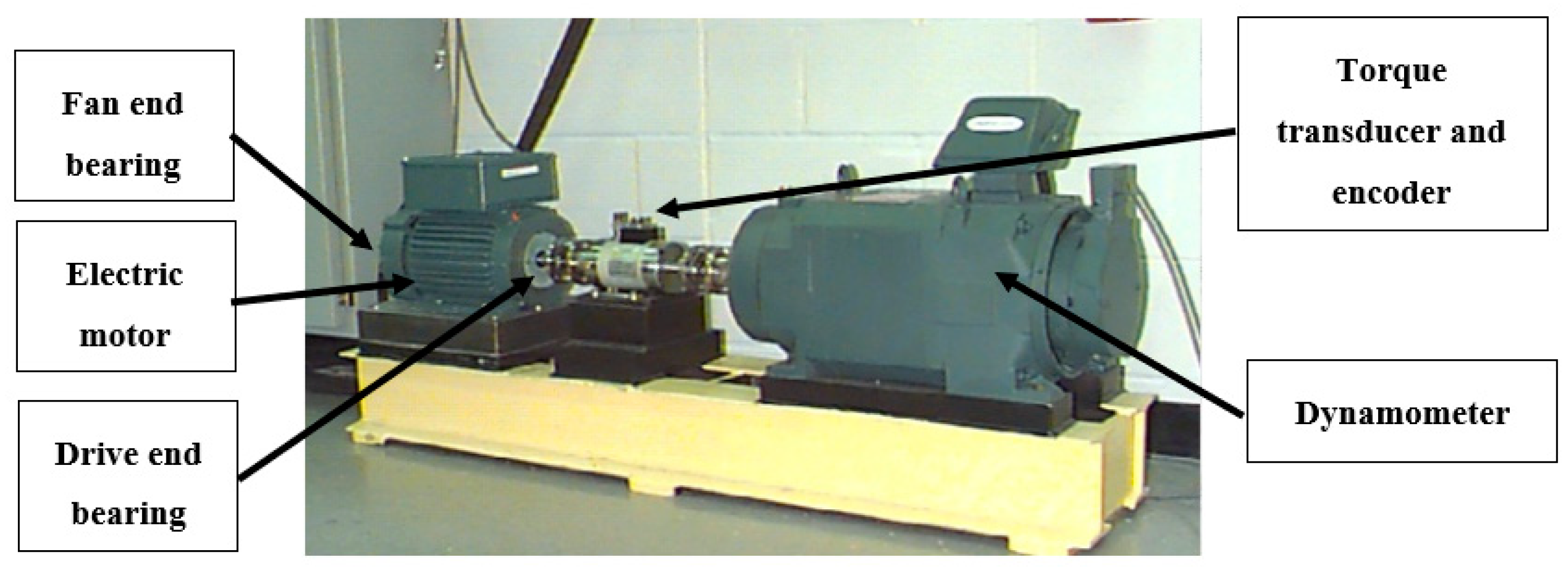
2.1. Case Western Reserve University Bearing Data Set (CWRU)

CWRU test apparatus (Figure 1) consists of a 2-hp electric motor, a torque transducer/encoder, dynamometer and control electronics. The motor shaft is supported by test ball bearings, indicated as fan end (FE) and drive end (DE) bearings. The specifications of the tested components are reported in

Table 1. Bearing specifications.

Bearing	Designation	BPFI—Multiple of Shaft Speed	${\mathit{P}}_{\mathit{u}}—\mathbf{Fatigue}\mathbf{Limits}\left(\mathbf{kN}\right)$
DE	SKF 6205-2RS JEM 1	5.415	0.335
FE	SKF 6203-2RS JEM	4.947	0.200

¹ NTN-equivalent bearings were used for 0.028 and 0.040 in drive end (DE) damages. FE: fan end and BPFI: Ball Passing Frequency on the Inner race.

.

Localized faults were introduced by means of an electro-discharge machining (EDM) on the inner race, outer race and balls with fault diameters varying from 0.007 to 0.040 in (0.18–1.02 mm). Defect depth was 0.011 in (0.28 mm) for diameters between 0.007 and 0.021 in, whereas it was 0.050 in (1.27 mm) for diameters of 0.028 and 0.040 in. The details of all the fault specifications are reported in [55]. In the present work, the case of an inner race damage introduced in the DE bearing was analyzed. In these circumstances, the damages with diameters of 0.007, 0.014 and 0.021 in (0.18, 0.35 and 0.53 mm) were considered, since they referred to the same bearing type (SKF 6205-2RS JEM). Tests were carried out for each damage level with the absorbed powers of 0, 1, 2 and 3 hp (0, 0.735, 1.470 and 2.205 kW). In these tests, the running speed N ranged between 1721 and 1796 rpm. Even though SI units (International System of Units) were preferred by the author of this work, they also chose to preserve coherence with the original work of the CWRU and with the extensive literature that relates to them.

Vibration data were collected using accelerometers fixed to the motor housing by means of a magnetic base at the 12 o’clock position (opposite to the load zone—6 o’clock position). The radial load, as pointed out by Smith and Randall [38], is mostly given by the static gravitational load. Baseline and fault-bearing signals were acquired using a 16-channel DAT recorder. Digital data handled in this study were sampled at 48 kHz (

Table 2. Vibration data specifications.

Damage Diameter (in)	Damage Depth (in)	Power (hp)	Fs—Sampling Frequency (kHz)	M—Number of Samples	T—Time Duration (s)
Baseline	Baseline	0-1-2-3	48	63,788	1.33
0.007(0.18 mm)	0.011(0.28 mm)	0-1-2-3	48	63,788	1.33
0.014(0.35 mm)	0.011(0.28 mm)	0-1-2-3	48	63,788	1.33
0.021(0.53 mm)	0.011(0.28 mm)	0-1-2-3	48	63,788	1.33

). Samples were preprocessed by extracting parts with equal time durations in order to take advantage of the automatable procedure adopted in this study. In this context, it was verified that the frequency resolution provided by the choice of the number of samples M was able to correctly represent the fast Fourier-transform (FFT) spectra. Furthermore, a reasonable number of fault impulses (more than 200) was contained in the time duration T.

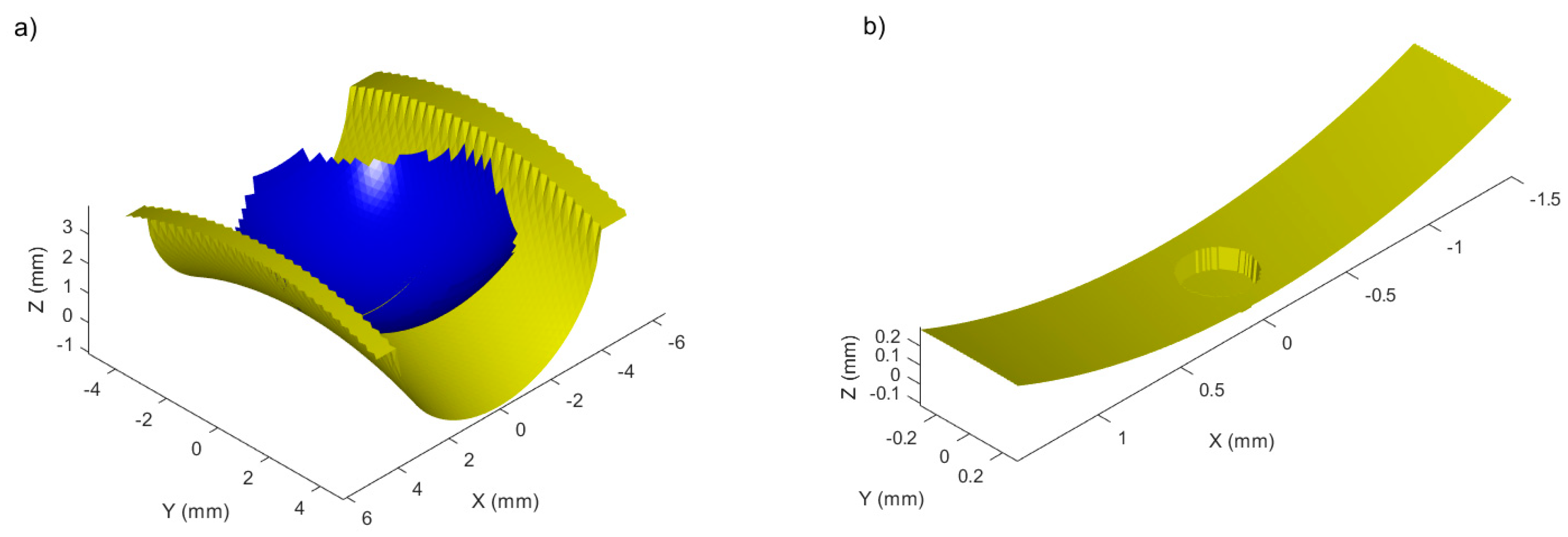
2.2. Non-Hertzian Contact Model

In order to obtain accurate pressure distributions, even in presence of a defect, a frictionless non-Hertzian numerical 3D surface contact model was used. This formulation was adopted since it is able to describe pressure distributions resulting from nonconstant curvatures and sudden geometry variations. Then, the discontinuities represented by defects are analyzed by means of this model. The contact conditions can be expressed in the so-called Hertz-Signorini-Moreau problem [61,62,63].

$$\mathit{h}\ge \mathbf{0},\hspace{1em}\hspace{1em}{\mathit{p}}_{\mathit{n}}\ge \mathbf{0},\hspace{1em}\hspace{1em}\mathit{h}·{\mathit{p}}_{\mathit{n}}=\mathbf{0}$$

(5)

The first condition enforces that no interpenetration can occur between the contact bodies, and therefore, the gap function $\mathit{h}$, which measures the distances between the surfaces, can only be positive or equal to $\mathbf{0}$ in the contact area. In Equation (5), and in the following, bold lowercase variables represent vectors, while bold uppercase variables represent matrices. The second condition imposes that the contact is nonadhesive, and therefore, no tension force can be present in the contact area formulated from the normal stress:

$${\mathit{\sigma }}_{\mathit{n}}=\mathit{t}\cdot \mathit{n}$$

(6)

where $\mathit{t}$ is the traction force vector, $\mathit{n}$ is the normal direction to the surface and ${\mathit{p}}_{\mathit{n}}=-{\mathit{\sigma }}_{\mathit{n}}$.

The third condition enforces that the normal pressures can only be different from $\mathbf{0}$ inside the contact area where $\mathit{h}=\mathbf{0}$ and null everywhere else. The gap function $\mathit{h}$ is expressed as

$$\mathit{h}=h_0+\mathit{g}+\mathit{\delta }$$

(7)

where $h_0$ is the indentation between the profiles imposed as a rigid body motion, $\mathit{g}$ is the initial separation of the contacting surfaces and represents its topography, while $\mathit{\delta }$ represents the elastic deformation of the surfaces due to the applied normal pressure ${\mathit{p}}_{\mathit{n}}$ and can be expressed as [64]

$$\mathit{\delta }=\mathit{C}\cdot {\mathit{p}}_{\mathit{n}}$$

(8)

where $\mathit{C}$ is a matrix of the influence coefficients, which introduces the elasticity of the contacting surfaces. Its components $C_{i,j} \left(i,j=0,1,\dots ,N\right)$ relate the displacement ${\delta }_i$ at a point $i$ due to the application of a unit pressure at point $j$.

The pressure distribution is estimated on the triangular grid-forming linearly varying pyramidal pressure elements, the definition of the influence coefficients $C_{i,j}$ is detailed in [65,66] and the solution procedure, which needs two iterative loops—one to eliminate tension forces and one to obtain the correct initial indentation $h_0$—is described in [54]. The computational model to which this contact algorithm will be applied is visible in Figure 2, alongside a detail of the representation of the geometry of the defect that will be introduced on the inner race for the reference size of 0.014 in (0.35 mm).

Although only gravitational loads were supposed, since no direct information regarding the actual load applied to the damaged bearing was given and the details regarding the apparatus, the motor and the related weights, three load levels were hypothesized to have more data to extrapolate from. Those load levels were inferred from the bearing specifics and, indeed, from the manufacturer of the bearing; the fatigue load limit is given as $P_u=335 \mathrm{N},$ and therefore, the force $F$ to be applied to the contact model was chosen as $F_1=\frac{1}{8}{P}_u, F_2=\frac{1}{4}{P}_u \mathrm{and} F_3=\frac{1}{2}{P}_u$. The experimental activity was conducted in such a way that only the gravitational load acted on the bearings, but the information about weights and motor specifications were not available. Therefore, the numerical signal was simulated by hypothesizing three load levels below the fatigue threshold and quite different among them. The first condition encompassed the assumption of an infinite life design, whereas the second enabled discussions on the variability of the diagnostic content with respect to the load level, as well as to damage the severity. Examples of the obtained pressure distributions for those force levels and different defect sizes are visible in Figure 3. Indeed, the pattern of the pressure distribution is Hertzian only when no defect is present in the contact area, while introducing the defect in the middle of the contact area introduces further overpressures, due to the sharp edges of the defect and the lack of material underneath the contact area. Furthermore, since the dimension of the damage is larger than the contact area, it produces two separate contact patterns in which the maximum pressure values are around three times higher than under normal conditions. The shape and the curvatures of the contact surfaces are simulated in the MATLAB^® code by referring to the bearing geometry specifications. The shapes and the sizes of the damages, for which an example is reported in Figure 2b, retrace the experimental data of Table 2. This model was then being used to extract the maximum contact pressure as a function of the rotation angle, numerically simulating around 100 revolutions in order to have a statistically significant sample, since the BPFI is not an integer with respect to a single revolution. Computations were carried out by simulating the relative motion between the race and the rolling element. No defect evolution due to plastic deformation was taken into account, since low loads and low numbers of cycles were simulated. The obtained time histories for three different load levels and damage dimensions are shown as examples in Figure 4 for the first few revolutions of the inner race.

Table 3. Contact pressure data specifications.

Damage Diameter (in)	Damage Depth (in)	Load—Fraction of Pu	Fs—Sampling Frequency (kHz)	M—Number of Samples	T—Time Duration (s)
0.007 (0.18 mm)	0.011 (0.28 mm)	1/8-1/4-1/2	48	63,788	1.33
0.014 (0.35 mm)	0.011 (0.28 mm)	1/8-1/4-1/2	48	63,788	1.33
0.021 (0.53 mm)	0.011 (0.28 mm)	1/8-1/4-1/2	48	63,788	1.33

reports the main features of the simulated contact pressure signals. The initial sampling frequency was rather high (74 kHz), given the fact that it was obtained numerically. Hence, the pressure signal was numerically resampled by means of interpolation and an antialiasing filter in order to make the damage detection analysis comparable with the experimental investigation. To the same end, numerical samples were cut by using M points.

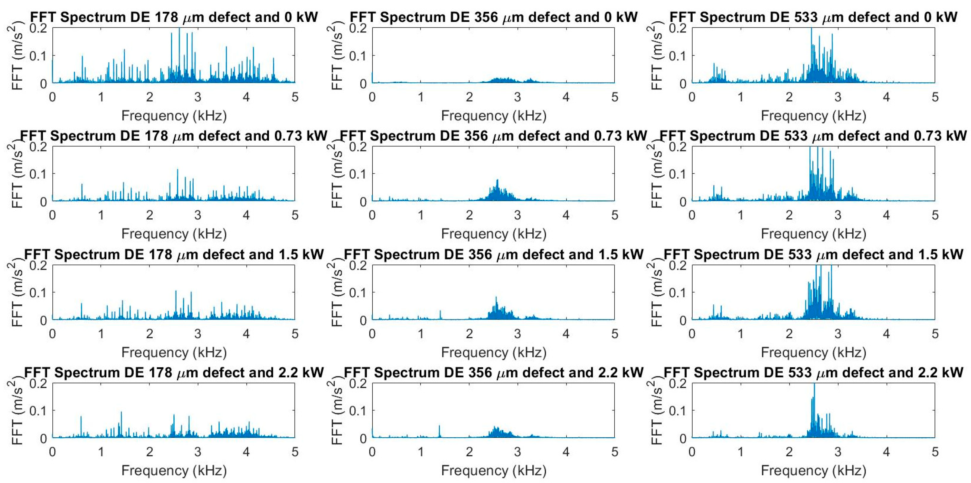
2.3. Damage Detection Analyisis

The damage detection analysis was carried out by taking advantage of the well-established concepts presented in the introduction to this work. Namely, different diagnostics features were extracted from both signals. Although the greatest part of these features enabled damage detectability, the fault severity assessment was not straightforward. Furthermore, it was a hardly identifiable correlation between the two signals in a diagnostic sense. For this reason, the authors proposed two health indicators to perform these tasks. Indeed, the dedicated features were constructed in an attempt to investigate direct correlations. Additionally, the conjectured sensitivity to the damage level was endorsed by the experimental validation. Vibration data coming from FE healthy bearing were analyzed as well. Prior to introducing the proposed indicators, the standard features and the methodology for their extraction are presented in the following.

• Time features (peak values, root mean square (RMS) and crest factor)
• Frequency features (mean contribution, xN harmonics and xBPFI harmonics)
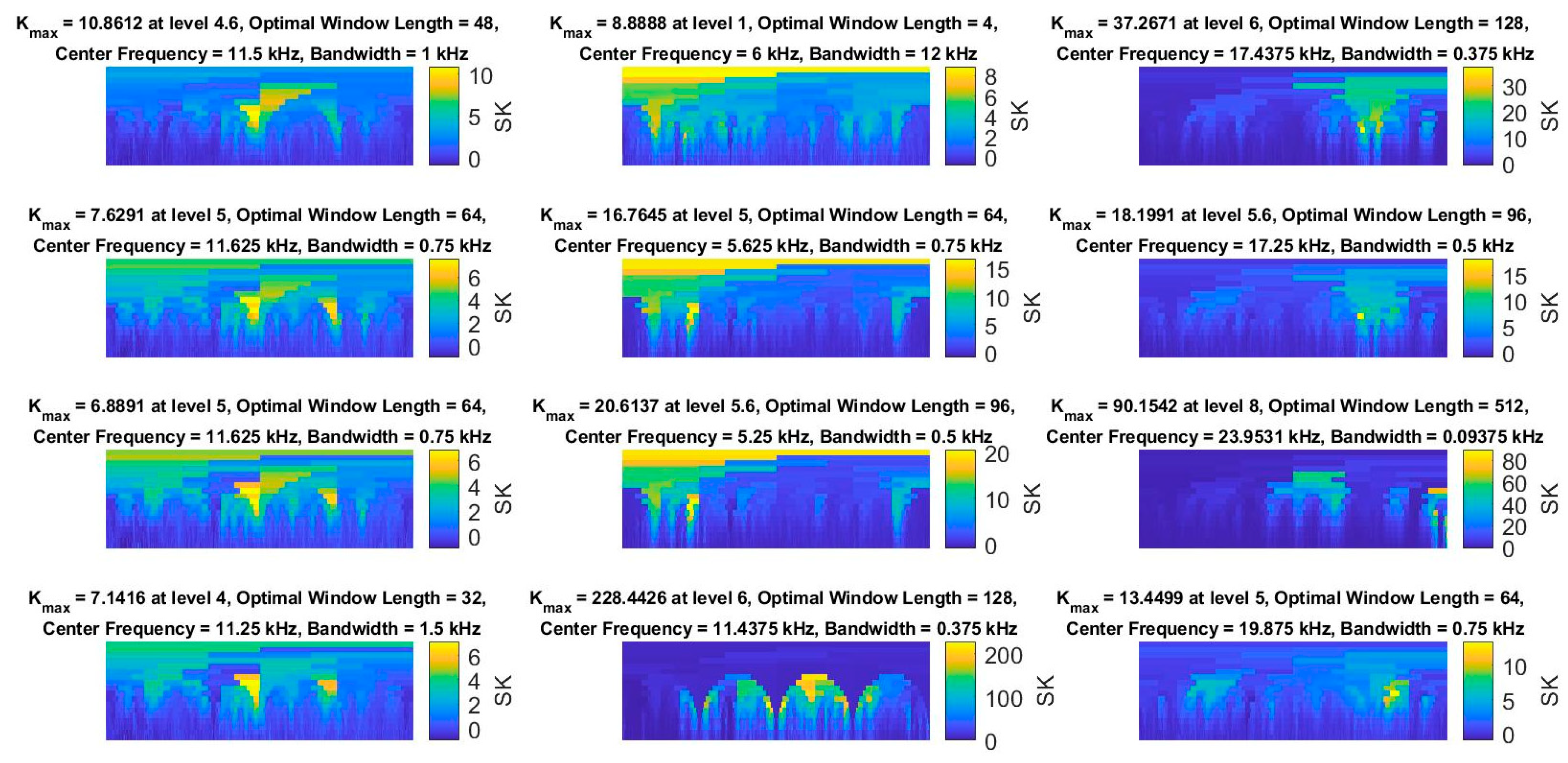
• Enhancement of the nonstationary part (SK and FK)
• Envelope extraction and signal demodulation (xBPFI harmonics of the demodulated signals)

Time domain and frequency domain features were investigated considering their variability linked to the damage severity and absorbed power (for the vibration signal) or applied load (for the pressure signal). Root mean square value (RMS), crest factor (CF) and kurtosis (K) are reported in Equations (9)–(11).

$$RMS=\sqrt{\frac{1}{T}{{\displaystyle \int }}_{-\infty }^{+\infty }{x}^2\left(t\right)dt}$$

(9)

$$CF=\frac{x_{peak}}{RMS}$$

(10)

$$K=\frac{E{\left(x-\mu \right)}^4}{{\sigma }^4}$$

(11)

where $T$ is the period, $x\left(t\right)$ is the time signal, $x_{peak}$ is the peak value of the signal, $E()$ is the expected value operator, $\mu$ is the mean value and $\sigma$ is the standard deviation. Kurtosis thus computed is expected to take the value of three for gaussian signals.

Frequency domain features were extracted from FFT raw spectra (Figure 5, Figure 6 and Figure 7). In particular, the mean contribution, the rotating contribution and the fault contribution, respectively corresponding to the 0-Hz harmonic, 1xN harmonic and 1xBPFI harmonic were individually analyzed.

SK and FK were employed for the purpose of enhancing the bearing signal in the vibration data and isolating the impulsive part in the pressure signal. As mentioned earlier, these methods are particularly useful, though many alternatives are available in the literature. Indeed, the potential filtering bands can be underlined by comparing power spectral densities (PSD) of undamaged and damaged bearings [1]. Nevertheless, a major problem with this method is that the machine signature needs always to be known. Besides, wavelet denoising [67,68,69] works by taking advantage of wavelet transform and deleting the wavelet contributions that go beyond a defined threshold. However, there are certain drawbacks associated with the use of this methodology, since the result strongly depends on the choice of the mother wavelet and of the thresholding method.

SK (Equation (12)) relies on the use of short-time Fourier transform (STFT) of Equation (13) to give a measure of the signal impulsiveness contained in frequency bands being examined.

$$SK=\frac{\langle \left|X^4\left(f,t\right)\right|\rangle }{{\langle \left|X\left(f,t\right)\right|}^2{\rangle }^2}-2$$

(12)

$$X\left(f,\tau \right)={{\displaystyle \int }}_{-\infty }^{+\infty }x\left(t\right)w\left(t-\tau \right)e^{-j2\pi ft}dt$$

(13)

where $\langle ·\rangle$ is the time-averaging operator, $X\left(f,t\right)$ is the time-frequency transform of the signal $x\left(t\right)$, $w\left(t-\tau \right)$ is a time window and $j$ is the imaginary unit.

The time-frequency representation of the signal is obtained by means of STFT, which, differently from FFT, is capable of localizing the harmonic contribution in time, since it is essentially a FFT that slides in time thanks to the window $w\left(t-\tau \right)$. SK is expected to be null for complex signals $X\left(f,\tau \right)$ originating from gaussian noises, whereas high values of SK suggest nonstationarity or non-gaussian properties. The size of the chosen window influences the SK computation, since STFT is affected by the well-known indetermination principle. Namely, the more accurate the time representation (short window), the worse the frequency resolution. For this reason, FK (Figure 8, Figure 9 and Figure 10) represents SK as a function of the window lengths. Therefore, FK provides information not only on the optimal demodulation band but, also, on the choice of the window length to be applied for the SK computation. Then, FK acts with a simplified algorithm, which avoids complete STFT computation.

Once signals were band pass-filtered in the frequency bands suggested by SK, the envelope analysis was applied. The modulus of the analytic signal was then investigated in the frequency domain (Figure 11). The xBPFI harmonic contributions were particularly examined. Unlike raw spectra, xBPFI harmonics were fairly identifiable even in the FE signal (Figure 12).

It is important to underline that the filtering process reduced the range in which the signals fluctuated. Moreover, this effect was different for each signal, given different filtering bands. Therefore, damage detectability cannot purely be assessed on the basis of the absolute value of the harmonic contributions but, rather, on their identifiability. Envelope spectrum was expected to show xBPFI harmonics, with sidebands spaced at the shaft rotation frequency. Clearly, this was mostly visible in the pressure signal, where no disturbance sources (noise or discrete harmonic components) were introduced.

The xBPFI harmonic contributions were analyzed for both signal envelopes and for all the damage levels and loads. However, none of these features for the enveloped and nonenveloped signals enabled a direct comparison between the diagnostic contents of the pressure and of the vibration signal, since these quantities, though linked, were intrinsically different. In an attempt to overcome this limitation, the novel step was introduced.

3. Proposed Health Indicators

The leading hypothesis behind the following argument is that the informative content on the damage severity is hidden beneath the energy related to the fault harmonics in the enveloped signals. To this purpose, the authors introduced the normalized power spectral density (NPSD) [42] obtained from the ratio between the PSD and the mean power of the signal, which is $RM{S}^2$ (Equations (14)–(16)).

$$E_x={{\displaystyle \int }}_{-\infty }^{+\infty }{x}^2\left(t\right)dt$$

(14)

$$RM{S}^2=\frac{1}{T}{{\displaystyle \int }}_{-\infty }^{+\infty }{x}^2\left(t\right)dt=\frac{E_x}{T}$$

(15)

$$NPSD\left(f\right)=\frac{PSD\left(f\right)}{RM{S}^2}$$

(16)

where $E_x$ is the signal energy.

One of the properties of the NPSD is that its integration in the frequency domain is unitary (Equation (17)).

$${{\displaystyle \int }}_{-\infty }^{+\infty }NPSD\left(f\right)df=1$$

(17)

Essentially, this is due to the fact that the integration of NPSD in a given frequency band results in the fraction of the signal power contained in such a band. Therefore, the health indicator (HI) proposed in Equation (18) gives an insight into the portion of power related to a frequency range with central frequency $f_c$ and bandwidth $\mathsf{\Delta }f$.

$$HI\left(f_c,\mathsf{\Delta }f\right)={{\displaystyle \int }}_{f_c-\frac{\mathsf{\Delta }f}{2}}^{f_c+\frac{\mathsf{\Delta }f}{2}}NPSD\left(f\right)df$$

(18)

Established that the conjunction between the SK and envelope analysis provided proper damage detectability into processed spectra, NPSD and HI were expected to give energetic information purely related to the fault, as long as they are evaluated in xBPFI harmonics. Indeed, thanks to NPSD and HI, the contribution given to the signal power solely imputable to the damage was investigated. This provided the remarkable possibility of isolating the contribution given to a global signal feature (mean power) by a very specific event, which is damage. Additionally, the physical significance of these features made the authors assume two interesting aspects. First, it was reasonable to hypothesize that the greater the defect size was, the more accentuated the relative energetic contribution given by the fault to the extracted signal. Hence, NPSD and HI were expected to be sensitive to damage severity. Secondly, the physical units of these quantities permitted a direct comparison between signals of different natures. Actually, the indicators referred to energetic quantities with respect to the total signal energy, which is different for each type of signal. Consequently, relative energetic features rather than absolute were adopted to compare different physical information in the pursuit of a correlation.

The described features were insofar evaluated in the xBPFI harmonics (

Table 4. Health indicator (HI) parameters.

Signal Type	$\mathbf{Frequency}\mathbf{Resolution}(\mathbf{Hz}){\mathit{f}}_{\mathit{r}\mathit{e}\mathit{s}}=\frac{{\mathit{f}}_{\mathit{s}}}{\mathit{M}}$	$\mathbf{Central}\mathbf{Frequency}{\mathit{f}}_{\mathit{c}}$	$\mathbf{Bandwidth}\mathsf{\Delta }\mathit{f}$$–\mathbf{Multiple}\mathbf{of}{\mathit{f}}_{\mathit{r}\mathit{e}\mathit{s}}$	$\mathbf{Bandwidth}\mathsf{\Delta }\mathit{f}\left(\mathbf{Hz}\right)$
Vibration	1.50	1xBPFI	8	12.03
Pressure	1.50	1xBPFI	8	12.03

) of the accelerometric and pressure signals, and the sensitivity to the load and damage level was explored.

Eventually, the correlation coefficient $r$ (Equation (19)) was considered as a measure of the linear dependence between the vibration and pressure features.

$$r=\frac{1}{P-1}{\displaystyle \sum }_{i=1}^P\left(\frac{F{P}_i-{\mu }_{FP}}{{\sigma }_{FP}}\right)\left(\frac{F{V}_i-{\mu }_{FV}}{{\sigma }_{FV}}\right)$$

(19)

where $P$ is the number of observations, $FP$ is the feature extracted from the pressure signal, ${\mu }_{FP}$ and ${\sigma }_{FP}$ are the mean and the standard deviation of $FP$, $FV$ is the feature extracted from the vibration signal and ${\mu }_{FV}$ and ${\sigma }_{FV}$ are the mean and the standard deviation of $FV$.

4. Methodology Application

As discussed previously, the aim of the study was to analyze the diagnostic content of two signals. The first is the vibration signal, which is commonly processed to extract information about bearings and machine health in a CBM perspective. The second is the contact pressure that arises between balls and race, since it is supposed to be one of the main sources of excitation in the dynamic equilibrium of the system. Therefore, the features presented in Section 2 are evaluated by means of the earlier described methodologies with the intention of comparing their diagnostic potential with that of the proposed health indicators. In most cases, although contact pressure analyses suggested smooth trends, vibration features showed to be hardly connectable to damage level and loads. Even more, a signals correlation was barely identifiable. Conversely, NPSD and HI showed to be appreciably sensitive to damage severity, and they paved the way for a direct comparison. In this section, the results of the application of the standard features and of the proposed indicators are presented.

4.1. Standard Features

Figure 13 shows the trend of the time features. DE and FE data showed similar patterns, but the effect of the damage level was not always clearly definable. Conversely, peak values and RMS of the contact pressure stem directly from the applied load and from the damage level. Indeed, the mean part of the pressure signal is influenced by the load, whereas the overpressure (Figure 4) comes from the effects of the defect size.

The frequency features of Figure 14 showed a similar behavior. The nonenveloped pressure signal manifested a smooth trend fairly suitable for damage level detection. Instead, the vibration data did not unequivocally show this attitude. Once more, the extracted features revealed were hardly relatable to the damage level and the diagnostic contents of the two physical signals placed on different levels.

Following the concepts reported in Section 2.3, signals were band pass-filtered in the frequency bands computed by means of FK. Most of the pressure signals revealed the maximum SK in a frequency band upper-circumscribed by the Nyquist limit. According to the authors, this was unavoidable, since the pressure signal showed very narrow peaks that resulted in wide frequency domain contents. Hence, most of the impulsivity was retained in the highest representable frequency bands. Differently, in the vibration signal, SK attempted to emphasize the bands where high-frequency structural resonances were excited by nonstationary phenomena, which were impacts of the rolling elements.

Subsequently, the envelope was extracted for signals demodulation. As can be seen from Figure 15, low values of the harmonic contents were appreciable in the first three xBPFI contributions. However, as pointed out in Section 2, an assessment based on the absolute values of such harmonics in enveloped signals may be misleading. One of the consequences of filtering in different bands according to the maximum SK criterion was to eradicate the similarity between DE and FE trends. Next, the xBPFI contents of the enveloped pressure signal were shown to be quite differently arranged with respect from the vibration analyses. The DE parameters were revealed to be not remarkably dependent on the damage level (Figure 15).

4.2. Proposed Health Indicators: Application to the Case-Study

NPSD and HI can be interpreted by visualizing their significance on FFT spectra. Figure 16 and Figure 17 report the example of the 0.021 in defect with 3 hp (vibration signal) and 0.021 and P_u/2 (contact pressure signal), but all the analyzed cases retraced this behavior. As long as the pressure signal is nonenveloped (Figure 16), most of the energetic content is concentrated in the low frequency range. The jumps in the cumulative NPSD point out the frequencies that mostly contribute to the signal PSD. Indeed, the very rapid increase detectable in the jumps corresponds to the harmonics in which the signal power is lumped. In particular, this occurred in the rotation frequency and xBPFI harmonics. When the pressure signal is enveloped, NPSD shows peaks corresponding to fault harmonics. This results in higher jumps in the cumulative NPSD. Raw vibration data did not exhibit this trend, since a great part of the signal power is given by resonance contributions. Conversely, it is interesting to notice that, in the enveloped vibration data (Figure 17), the energetic jumps are mostly related to the xBPFI content. This is consistent with the extensive literature supporting the strength of the envelope analysis for damage detectability [1,22,23,35,37,70]. NPSD and cumulative NPSD were computed for nonenveloped and enveloped signals considering all the loads and damage level cases.

The HI proposed in Equation (18) provides a quantitative extent of the jumps, since it represents the fraction of the power contained in these gaps relative to the whole signal power. As anticipated, it was hypothesized that the higher this fraction is, the more accentuated the damage severity, since a greater part of the signal energy is relatable to the presence of the fault. It appeared that this assumption was valid for the pressure signal, in which it was found a linear trend of NPSD and HI with respect to the defect size (Figure 18). As expected, the indicators, though showing a similar trend, exhibited lower values for the nonenveloped signal.

Figure 19 shows the trend of these features for the enveloped and raw DE and FE signals. It can be observed that the damage is hardly detectable by means of these indicators without demodulation. On the other hand, in the enveloped signals, it is possible to allocate up to 20% of the signal power to the presence of localized faults. Interestingly, these values are comparable with the FE signal, since the adopted indicators are normalized with respect to the properties of each signal. Hence, in FE signals, low power fractions are related to low signal powers, resulting in values comparable with DE ones. Differently from K and CF, which have neutral physical units in the same way, NPSD and HI assume similar values in the vibration and in the pressure signal. Indeed, NPSD and HI refer to the relation between an isolated event (damage) and signal power, whereas K and CF globally measure the effect of the damage on the time domain shape.

5. Methodology Validation

In order to investigate the feature sensitivity to the damage severity, the indicators were analyzed by considering multiple powers or applied loads as different realizations of a given damage level. The boxplots of Figure 20 indicate the attitudes of the different features for the three damage levels: L1, L2 and L3, which correspond, respectively, to 0.007, 0.014 and 0.021 in. It appears that, for all the feature distributions, it is slightly identifiable as a clear distinction between damage levels, except for NPSD and HI, which emphasize an evident discrimination. This reinforces the original assumption taken for the construction of NPSD and HI and confirms that, actually, the power fraction merely imputable to the presence of the defect is very sensitive to damage severity. However, boxplots are employed to give a graphical representation of the data, but their significance must be consolidated by a larger amount of realizations for each damage level.

Detectability is studied by adopting the same approach even for the baseline and fault analysis performed on the vibration data, validating the capabilities of the proposed Indicators. As shown in Figure 21 and Figure 22, all the features are able to discern faulty bearings, with the exception of the central frequency of the maximum SK band. Evidently, this feature is related to the research of nonstationarity, and no linear trend is expected between this parameter and damage severity. A clear separation between indicators for different damage levels is not identifiable for all the features. However, kurtosis (K) showed an increasing trend with well-separable distributions related to different damage levels.

Interestingly, the NPSD and HI were revealed to be promising features, since they fulfilled three main criteria. First, they can classify faulty bearings with respect to healthy ones. Secondly, they assume an increasing trend with respect to the damage level. Finally, their boxplots do not suffer excessive superimposition. Nevertheless, only a larger amount of data will confirm this attitude. One of the extremely attractive features of NPSD and HI is their values in the pressure signal and in the experimental signal of the damaged-bearing range in similar intervals for each fault size. Given the fact that NPSD and HI are endowed with neutral physical units, the diagnostic correlation between contact pressure and vibration was investigated (Figure 23).

Figure 23 shows the results of the correlation study carried out by means of Equation (19) described in Section 3. The mean value of the damage-related power HI and of NPSD are computed for each fault level. These values constitute the $FP$ and $FV$ of Equation (19). The noteworthy correlation coefficients (

Table 5. Correlation coefficients. NPSD: normalized power spectral density.

Health Indicator	r—Correlation Coefficient	R2—Coefficient of Determination
HI—damage-related power	0.89	0.79
NPSD	0.96	0.92

) confirm these indicators to provide an evaluable key to link two different quantities from a diagnostic content perspective. This evidence reinforces the initial idea that one of the sources generating the dynamic response is actually related to this latter in a diagnostic sense. Moreover, it is found that, by taking into account diagnostic quantities, the possible correlation lies in the signal power. Indeed, this study highlights that the signal power strictly related to the damage is sensitive to fault dimensions.

6. Discussion and Conclusions

This work documents the diagnostic analysis carried out on faulty and healthy bearings of a CWRU vibration dataset. Namely, previous research contributions have drawn attention on SK for the enhancement of nonstationarity and on the envelope analysis for signal demodulation. No less research in bearing diagnostics is devoted to feature extraction methods based on data-driven models. However, in this study, the authors placed emphasis on physical phenomena underpinning the resulting experimental data, thus preferring diagnostic methodologies that do not suffer from an excessive detachment from physics-based considerations, which may help data interpretation. Moreover, these techniques are applied to evaluate the capability of damage severity assessments for different diagnostic features. To this aim, the diagnostic content was analyzed both in a numerical and in an experimental signal. The numerical signal was generated by investigating the contact pressure established between the balls and the defected race. Indeed, the contact pressure was supposed to be one of the main sources of excitation in the system dynamic response.

Therefore, envelope analysis was applied to extract features and evaluate their damage level sensitivity. The choice of the demodulation band was assisted by FK, which enabled the enhancement of the bearing signal in the vibration data, whereas, in the numerical signal, it contributed to the isolation of the impulsive phenomena.

Actually, out an inherent difference between the two signals must be pointed out. In the vibration spectrum, fault harmonics are buried due to the excitation of high-frequency structural resonances and SK acts by bringing to light the bands in which the nonstationary part is hidden. On the contrary, the numerical signal is not influenced by the structural dynamics of the whole test rig, and the peaks do not suffer from damping flattening. Therefore, FK emphasizes impulses that, however, are not completely undetectable in raw spectra.

Two health indicators were introduced. They were constructed relying on the assumption that the more severe the damage, the more the signal power strictly relatable to faults is accentuated. In the attempt of isolating this contribution, SK and envelope extraction were applied, resorting to their physical significance. The indicators showed their attitude in identifying faulty bearings with respect to healthy ones. Moreover, the results showed that they may be capable of assessing the damage severity as well. Another compelling aspect is that their physical units are neutral, paving the way for a comparison between the diagnostic contents of the source, which is the pressure signal, and the effect, represented by the vibration data. Indeed, when these signals are evaluated through the mentioned indicators, a correlation is found. Therefore, it is concluded that the energetic indicators may be proposed for damage detection and damage level assessment but, also, as reading keys of a correlation between the vibration and the pressure signal. One of the drawbacks of these indicators is that they precisely point the xBPFI harmonic contents, relying on the detectability of a significant harmonic contribution in these frequencies.

However, these analyses were carried out by considering a limited amount of data, both in terms of the fault level and applied loads. Then, future works should include more data in order to validate and give statistical significance to these considerations. Other fault types should also be investigated, together with the possible prognostic capabilities. The use of different diagnostic methodologies, such as alternatives to FK, squared envelope and data-driven models, could be investigated as well.

References

1. Randall, R.B. Vibration-Based Condition Monitoring: Industrial, Aerospace and Automotive Applications; John Wiley & Sons: Hoboken, NJ, USA, 2011; ISBN 9780470747858. [Google Scholar]
2. Mohanty, A.R. Machinery Condition Monitoring: Principles and Practices; CRC Press: Boca Raton, FL, USA, 2014; ISBN 9781466593053. [Google Scholar]
3. Woodley, B.J. Failure prediction by condition monitoring (part 1). Int. J. Mater. Eng. Appl. 1978, 1, 19–26. [Google Scholar] [CrossRef]
4. Jia, F.; Lei, Y.; Lin, J.; Zhou, X.; Lu, N. Deep neural networks: A promising tool for fault characteristic mining and intelligent diagnosis of rotating machinery with massive data. Mech. Syst. Signal Process. 2016. [Google Scholar] [CrossRef]
5. Ben Ali, J.; Saidi, L.; Mouelhi, A.; Chebel-Morello, B.; Fnaiech, F. Linear feature selection and classification using PNN and SFAM neural networks for a nearly online diagnosis of bearing naturally progressing degradations. Eng. Appl. Artif. Intell. 2015, 42, 67–81. [Google Scholar] [CrossRef] [Green Version]
6. Tabrizi, A.; Garibaldi, L.; Fasana, A.; Marchesiello, S. Early damage detection of roller bearings using wavelet packet decomposition, ensemble empirical mode decomposition and support vector machine. Meccanica 2015, 50, 865–874. [Google Scholar] [CrossRef]
7. Daga, A.P.; Fasana, A.; Marchesiello, S.; Garibaldi, L. The Politecnico di Torino rolling bearing test rig: Description and analysis of open access data. Mech. Syst. Signal Process. 2019, 120, 252–273. [Google Scholar] [CrossRef]
8. Jin, X.; Chow, T.W.S. Anomaly detection of cooling fan and fault classification of induction motor using Mahalanobis-Taguchi system. Expert Syst. Appl. 2013, 40, 5787–5795. [Google Scholar] [CrossRef]
9. Jin, X.; Wang, Y.; Chow, T.W.S.; Sun, Y. MD-based approaches for system health monitoring: A review. IET Sci. Meas. Technol. 2017, 11, 371–379. [Google Scholar] [CrossRef]
10. Shakya, P.; Kulkarni, M.S.; Darpe, A.K. Bearing diagnosis based on Mahalanobis-Taguchi-Gram-Schmidt method. J. Sound Vib. 2015, 337, 342–362. [Google Scholar] [CrossRef]
11. Shen, C.; Wang, D.; Kong, F.; Tse, P.W. Fault diagnosis of rotating machinery based on the statistical parameters of wavelet packet paving and a generic support vector regressive classifier. Meas. J. Int. Meas. Confed. 2013, 46, 1551–1564. [Google Scholar] [CrossRef]
12. Yang, J.; Zhang, Y.; Zhu, Y. Intelligent fault diagnosis of rolling element bearing based on SVMs and fractal dimension. Mech. Syst. Signal Process. 2007, 21, 2012–2024. [Google Scholar] [CrossRef]
13. Liu, R.; Yang, B.; Zio, E.; Chen, X. Artificial intelligence for fault diagnosis of rotating machinery: A review. Mech. Syst. Signal Process. 2018, 108, 33–47. [Google Scholar] [CrossRef]
14. Pinheiro, A.A.; Brandao, I.M.; Da Costa, C. Vibration Analysis in Turbomachines Using Machine Learning Techniques. Eur. J. Eng. Res. Sci. 2019, 4, 12–16. [Google Scholar] [CrossRef] [Green Version]
15. Wang, D.; Tse, P.W.; Guo, W.; Miao, Q. Support vector data description for fusion of multiple health indicators for enhancing gearbox fault diagnosis and prognosis. Meas. Sci. Technol. 2011, 22. [Google Scholar] [CrossRef] [Green Version]
16. Baccarini, L.M.R.; Rocha e Silva, V.V.; de Menezes, B.R.; Caminhas, W.M. SVM practical industrial application for mechanical faults diagnostic. Expert Syst. Appl. 2011, 38, 6980–6984. [Google Scholar] [CrossRef]
17. Widodo, A.; Yang, B.-S. Support vector machine in machine condition monitoring and fault diagnosis. Mech. Syst. Signal Process. 2007, 21, 2560–2574. [Google Scholar] [CrossRef]
18. Liu, Z.; Cao, H.; Chen, X.; He, Z.; Shen, Z. Multi-fault classification based on wavelet SVM with PSO algorithm to analyze vibration signals from rolling element bearings. Neurocomputing 2013, 99, 399–410. [Google Scholar] [CrossRef]
19. Mba, D. The use of acoustic emission for estimation of bearing defect size. J. Fail. Anal. Prev. 2008, 8, 188–192. [Google Scholar] [CrossRef]
20. Al-Dossary, S.; Hamzah, R.I.R.; Mba, D. Observations of changes in acoustic emission waveform for varying seeded defect sizes in a rolling element bearing. Appl. Acoust. 2009, 70, 58–81. [Google Scholar] [CrossRef] [Green Version]
21. Al-Ghamd, A.M.; Mba, D. A comparative experimental study on the use of acoustic emission and vibration analysis for bearing defect identification and estimation of defect size. Mech. Syst. Signal Process. 2006, 20, 1537–1571. [Google Scholar] [CrossRef] [Green Version]
22. Randall, R.B.; Antoni, J. Rolling element bearing diagnostics-A tutorial. Mech. Syst. Signal Process. 2011, 25, 485–520. [Google Scholar] [CrossRef]
23. Sawalhi, N.; Randall, R.B. Semi-automated bearing diagnostic-three case studies. Non Destrcutive Test. Aust. 2008, 45, 59. [Google Scholar]
24. Abboud, D.; Elbadaoui, M.; Smith, W.A.; Randall, R.B. Advanced bearing diagnostics: A comparative study of two powerful approaches. Mech. Syst. Signal Process. 2019, 114, 604–627. [Google Scholar] [CrossRef]
25. Wang, D.; Tsui, K.-L.; Miao, Q. Prognostics and Health Management: A Review of Vibration Based Bearing and Gear Health Indicators. IEEE Access 2018, 6, 665–676. [Google Scholar] [CrossRef]
26. Sinha, J.K.; Elbhbah, K. A future possibility of vibration based condition monitoring of rotating machines. Mech. Syst. Signal Process. 2013, 34, 231–240. [Google Scholar] [CrossRef]
27. Rai, A.; Upadhyay, S.H. A review on signal processing techniques utilized in the fault diagnosis of rolling element bearings. Tribol. Int. 2016. [Google Scholar] [CrossRef]
28. De Azevedo, H.D.M.; Araújo, A.M.; Bouchonneau, N. A review of wind turbine bearing condition monitoring: State of the art and challenges. Renew. Sustain. Energy Rev. 2016, 56, 368–379. [Google Scholar] [CrossRef]
29. Genta, G. Dynamics of Rotating Systems; Springer Science & Business Media: Berlin, Germany, 2007. [Google Scholar]
30. Genta, G.; Delprete, C.; Brusa, E. Some considerations on the basic assumptions in rotordynamics. J. Sound Vib. 1999, 227, 611–645. [Google Scholar] [CrossRef]
31. Burchill, R.F.; John, L.F.; Wilson, D.S. New Machinery Health Diagnostic Techniques Using High-Frequency Biration; SAE Technical Paper; SAE International: Warrendale, PA, USA, 1973. [Google Scholar]
32. Burchill, R.F. Resonant structure techniques for bearing fault analysis. Natl. Bur. Stand. NBSIR 1973, 73, 252. [Google Scholar]
33. Darlow, M.; Badgley, R.H. Early Detection of Defects in Rolling-Element Bearings; SAE Technical Paper; SAE International: Warrendale, PA, USA, 1975. [Google Scholar]
34. Harting, D.R. Demodulated resonance analysis—A powerful incipient failure detection technique. ISAT 1978, 17, 35–40. [Google Scholar]
35. McFadden, P.D.; Smith, J.D. Vibration monitoring of rolling element bearings by the high-frequency resonance technique—A review. Tribol. Int. 1984, 17, 3–10. [Google Scholar] [CrossRef]
36. McFadden, P.D.; Smith, J.D. Model for the vibration produced by a single point defect in a rolling element bearing. J. Sound Vib. 1984, 96, 69–82. [Google Scholar] [CrossRef]
37. Rubini, R.; Meneghetti, U. Application of the envelope and wavelet transform analyses for the diagnosis of incipient faults in ball bearings. Mech. Syst. Signal Process. 2001, 15, 287–302. [Google Scholar] [CrossRef]
38. Smith, W.A.; Randall, R.B. Rolling element bearing diagnostics using the Case Western Reserve University data: A benchmark study. Mech. Syst. Signal Process. 2015, 64–65, 100–131. [Google Scholar] [CrossRef]
39. Randall, R.B.; Antoni, J.; Chobsaard, S. The relationship between spectral correlation and envelope analysis in the diagnostics of bearing faults and other cyclostationary machine signals. Mech. Syst. Signal Process. 2001, 15, 945–962. [Google Scholar] [CrossRef]
40. Mauricio, A.; Smith, W.; Randall, R.B.; Antoni, J.; Gryllias, K. Cyclostationary-based tools for bearing diagnostics. In Proceedings of the ISMA 2016 Including USD, Leuven, Belgium, 19–21 September 2016; pp. 905–918. [Google Scholar]
41. Delprete, C.; Milanesio, M.; Rosso, C. Rolling bearings monitoring and damage detection methodology. Appl. Mech. Mater. 2005, 3–4, 293–302. [Google Scholar] [CrossRef]
42. Brusa, E.; Bruzzone, F.; Delprete, C.; Di Maggio, L.G.; Rosso, C. A Proposal of a Technique for Correlating Defect Dimensions to Vibration Amplitude in Bearing Monitoring. In Proceedings of the PHM Society European Conference, Turin, Italy, 27–31 July 2020; pp. 1–14. [Google Scholar]
43. Delprete, C.; Brusa, E.; Rosso, C.; Bruzzone, F. Bearing Health Monitoring Based on the Orthogonal Empirical Mode Decomposition. Shock Vib. 2020, 2020. [Google Scholar] [CrossRef]
44. Antoni, J.; Randall, R.B. The spectral kurtosis: Application to the vibratory surveillance and diagnostics of rotating machines. Mech. Syst. Signal Process. 2006, 20, 308–331. [Google Scholar] [CrossRef]
45. Antoni, J. The spectral kurtosis of nonstationary signals: Formalisation, some properties, and application. In Proceedings of the 2004 12th European Signal Processing Conference, Vienna, Austria, 6–10 September 2004; IEEE: Piscataway, NJ, USA, 2015; pp. 1167–1170. [Google Scholar]
46. Antoni, J. The spectral kurtosis: A useful tool for characterising non-stationary signals. Mech. Syst. Signal Process. 2006, 20, 282–307. [Google Scholar] [CrossRef]
47. Antoni, J. Fast computation of the kurtogram for the detection of transient faults. Mech. Syst. Signal Process. 2007, 21, 108–124. [Google Scholar] [CrossRef]
48. Wang, D. Some further thoughts about spectral kurtosis, spectral L2/L1 norm, spectral smoothness index and spectral Gini index for characterizing repetitive transients. Mech. Syst. Signal Process. 2018, 108, 58–72. [Google Scholar] [CrossRef]
49. Wang, D. Spectral L2/L1 norm: A new perspective for spectral kurtosis for characterizing non-stationary signals. Mech. Syst. Signal Process. 2018, 104, 290–293. [Google Scholar] [CrossRef]
50. Moshrefzadeh, A.; Fasana, A. The Autogram: An effective approach for selecting the optimal demodulation band in rolling element bearings diagnosis. Mech. Syst. Signal Process. 2018. [Google Scholar] [CrossRef]
51. Antoni, J. The infogram: Entropic evidence of the signature of repetitive transients. Mech. Syst. Signal Process. 2016, 74, 73–94. [Google Scholar] [CrossRef]
52. Bonnardot, F.; Randall, R.B. Enanched unsupervised noise cancellation using angular resampling for planetary bearing fault diagnosis. Int. J. Acoust. Vib. 2004, 9, 51–60. [Google Scholar]
53. Abboud, D.; Antoni, J.; Sieg-Zieba, S.; Eltabach, M. Envelope analysis of rotating machine vibrations in variable speed conditions: A comprehensive treatment. Mech. Syst. Signal Process. 2017, 84, 200–226. [Google Scholar] [CrossRef]
54. Marmo, F.; Toraldo, F.; Rosati, A.; Rosati, L. Numerical solution of smooth and rough contact problems. Tribol. Int. 2018, 53, 1415–1440. [Google Scholar] [CrossRef]
55. Case Western Reserve University Bearing Data Center Website. Available online: https://csegroups.case.edu/bearingdatacenter/pages (accessed on 3 August 2020).
56. Li, Y.; Xu, M.; Wei, Y.; Huang, W. A new rolling bearing fault diagnosis method based on multiscale permutation entropy and improved support vector machine based binary tree. Meas. J. Int. Meas. Confed. 2016, 77, 80–94. [Google Scholar] [CrossRef]
57. Lei, Y.; He, Z.; Zi, Y. A new approach to intelligent fault diagnosis of rotating machinery. Expert Syst. Appl. 2008, 35, 1593–1600. [Google Scholar] [CrossRef]
58. Liu, H.; Han, M. A fault diagnosis method based on local mean decomposition and multi-scale entropy for roller bearings. Mech. Mach. Theory 2014, 75, 67–78. [Google Scholar] [CrossRef]
59. Li, W.; Qiu, M.; Zhu, Z.; Wu, B.; Zhou, G. Bearing fault diagnosis based on spectrum images of vibration signals. Meas. Sci. Technol. 2016, 27. [Google Scholar] [CrossRef] [Green Version]
60. Li, B.; Zhang, Y. Supervised locally linear embedding projection (SLLEP) for machinery fault diagnosis. Mech. Syst. Signal Process. 2011, 25, 3125–3134. [Google Scholar] [CrossRef]
61. Johnson, K.L. Contact Mechanics; Cambridge University Press: Cambridge, UK, 1987. [Google Scholar]
62. Kalker, J.J. Three-Dimensional Elastic Bodies in Rolling Contact; Springer: Berlin, Germany, 1990. [Google Scholar]
63. Wriggers, P. Computational Contact Mechanics; Springer: Berlin, Germany, 2002. [Google Scholar]
64. Sayles, R.S. Basic principles of rough surface rough contact analysis using numerical methods. Tribol. Int. 1996, 29, 639–650. [Google Scholar] [CrossRef]
65. Kalker, J.J.; Van Randen, Y. A minimum principle for frictionless elastic contact with application to non-Hertzian half-space contact problems. J. Eng. Math. 1972, 6, 193–206. [Google Scholar] [CrossRef]
66. Boedo, S. A corrected displacement solution to linearly varying surface pressure over a triangular region on the elastic half-space. Tribol. Int. 2013, 60, 116–118. [Google Scholar] [CrossRef]
67. Donoho, D.L.; Johnstone, J.M. Ideal spatial adaptation by wavelet shrinkage. Biometrika 1994, 81, 425–455. [Google Scholar] [CrossRef]
68. Qiu, H.; Lee, J.; Lin, J.; Yu, G. Wavelet filter-based weak signature detection method and its application on rolling element bearing prognostics. J. Sound Vib. 2006, 289, 1066–1090. [Google Scholar] [CrossRef]
69. Wang, D.; Tse, P.W.; Tsui, K.-L. An enhanced Kurtogram method for fault diagnosis of rolling element bearings. Mech. Syst. Signal Process. 2013, 35, 176–199. [Google Scholar] [CrossRef]
70. Guo, Y.; Liu, T.-W.; Na, J.; Fung, R.-F. Envelope order tracking for fault detection in rolling element bearings. J. Sound Vib. 2012, 331, 5644–5654. [Google Scholar] [CrossRef]
Figure 1. Case Western Reserve University (CWRU) bearings test apparatus [38,55].
Applsci 10 08131 g001
Figure 2. (a) Computational model of the inner race and ball. (b) Detail of the damaged inner race for a defect size of 0.014 in (0.35 mm).
Applsci 10 08131 g002
Figure 3. Examples of contact pressure distributions at different load levels and defect sizes.
Applsci 10 08131 g003
Figure 4. Examples of the computed time histories for different load levels and defect sizes.
Applsci 10 08131 g004
Figure 5. Fast Fourier-transform (FFT) raw spectra: vibration signals. DE: drive end.
Applsci 10 08131 g005
Figure 6. FFT raw spectra: pressure signals.
Applsci 10 08131 g006
Figure 7. FFT raw spectra: (a) vibration signal, (b) pressure signal, (c) vibration signal up to 5 kHz and (d) pressure signal up to 5 kHz.
Applsci 10 08131 g007
Figure 8. Kurtograms: (a) vibration signal at 0.021 in and 3 hp and (b) pressure signal at 0.021 in and Pu/2.
Applsci 10 08131 g008
Figure 9. Kurtograms: vibration signals. The three columns refer, respectively, to 0.007, 0.014 and 0.021 in. The four rows refer, respectively, to 0, 1, 2 and 3 hp.
Applsci 10 08131 g009
Figure 10. Kurtograms: pressure signals. The three columns refer, respectively, to 0.007, 0.014 and 0.021 in. The three rows refer, respectively, to Pu/8, Pu/4 and Pu/2.
Applsci 10 08131 g010
Figure 11. Envelope signal and envelope spectrum: (a) vibration signal at 0.021 in and 3 hp and (b) pressure signal at 0.021 in and Pu/2. In red, the first ten xBPFI harmonics. BPFI: Ball Passing Frequency on the Inner race.
Applsci 10 08131 g011
Figure 12. Envelope signal and envelope spectrum. Fan end (FE) signal with damage on DE bearing. In red, the first ten xBPFI harmonics.
Applsci 10 08131 g012
Figure 13. Time features analysis for contact pressure, DE and FE signals.
Applsci 10 08131 g013
Figure 14. Frequency features analysis for contact pressure, DE and FE signals.
Applsci 10 08131 g014
Figure 15. xBPFI contents for contact pressure, DE and FE enveloped signals.
Applsci 10 08131 g015
Figure 16. Normalized power spectral density (NPSD) and cumulative NPSD nonenveloped and enveloped signals: pressure signal.
Applsci 10 08131 g016
Figure 17. NPSD and cumulative NPSD nonenveloped and enveloped signals: vibration signal.
Applsci 10 08131 g017
Figure 18. NPSD and health indicator (HI) for the enveloped and nonenveloped pressure signal.
Applsci 10 08131 g018
Figure 19. NPSD and HI for the enveloped and nonenveloped vibration signals. (a) DE and (b) FE.
Applsci 10 08131 g019
Figure 20. Boxplots for the features extracted from the pressure signal: (a) peak value, root mean square (RMS), crest factor (CF) and kurtosis (K) and (b) central frequency of the maximum spectral kurtosis (SK) band, 1xBPFI content in the NPSD and HI in the 1xBPFI.
Applsci 10 08131 g020
Figure 21. Boxplots for the features extracted from the vibration signal: peak value, RMS, CF and K.
Applsci 10 08131 g021
Figure 22. Boxplots for the features extracted from the vibration signal: central frequency of the maximum SK band, 1xBPFI content in the NPSD and HI in the 1xBPFI.
Applsci 10 08131 g022
Figure 23. Correlation between the pressure and vibration signals by means of HI and NPSD.
Applsci 10 08131 g023