Compact Spatial Pyramid Pooling Deep Convolutional Neural Network Based Hand Gestures Decoder

 ,
, 
Abstract
1. Introduction
2. Related Works
3. Basic Theory for Optimizing DCNN
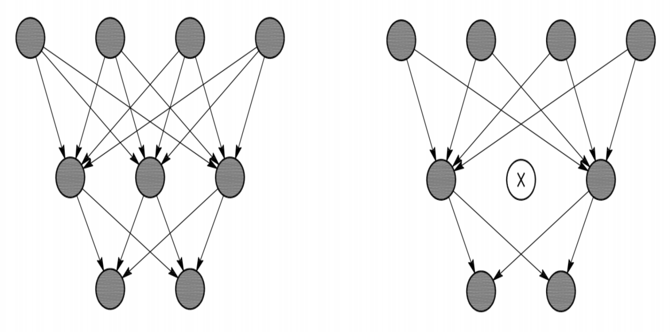
3.1. Deep Convolutional Neural Network and Node Pruning
3.2. Image Resizing Restriction in DCNN
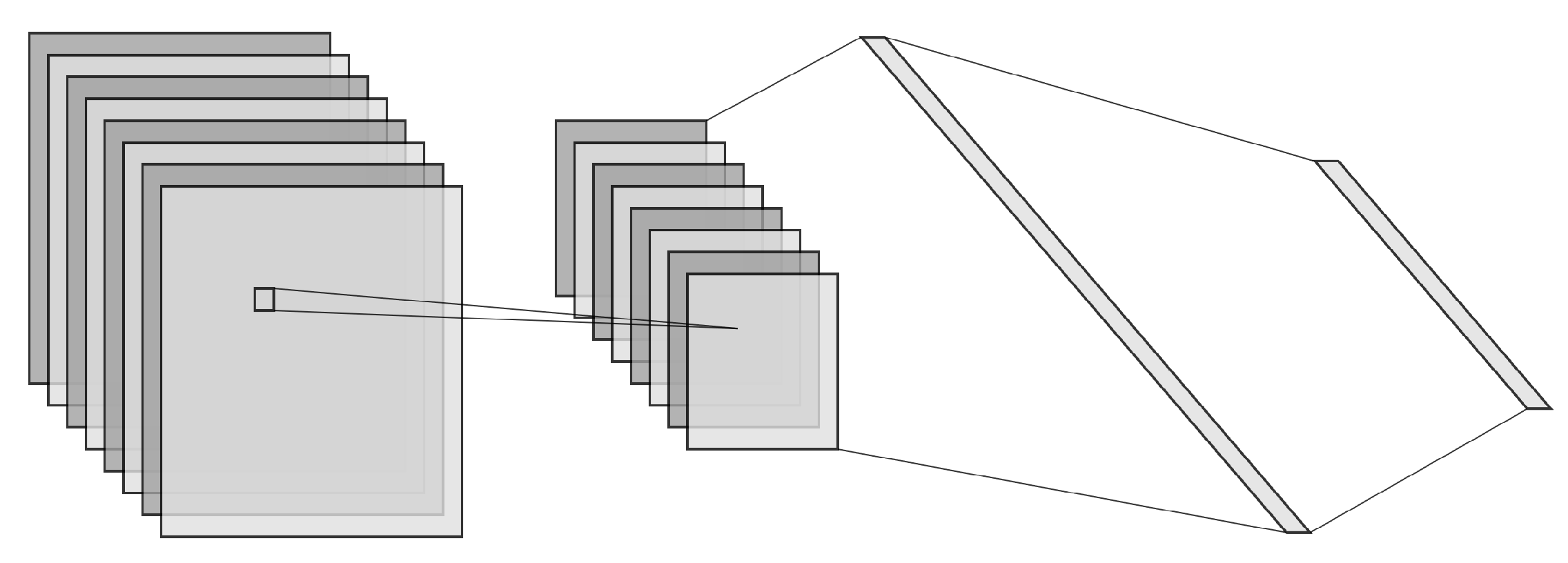
3.3. Spatial Pyramid Pooling Layer (SPP)
4. The Proposed Methodology
4.1. Practical DCNN Architecture Selection and Pruning Strategy for Optimal Node Selection
4.2. Integration of Multi-Spatial Pyramid Pooling into the Pruned DCNN
4.3. Practical Classification Algorithm for Real-Time Gesture-To-Word Decoding
| Algorithm 1 Hand Gesture Decoding Algorithm |
Input: Hand gesture video or image frames set Output: Decoded alphabets instruction set BEGIN Step 1: Process the video for the given frames per second (fps) Step 2: Transform the images as 2D array where M is fps and the N will be the instruction/word length (images) Step 3: Apply the Proposed Compact Spatial Pyramid Pooling Deep Convolutional Neural Network to transform each images Step 4: Column wise Majority Selection Step 5: Return array of n-sized output instruction END |
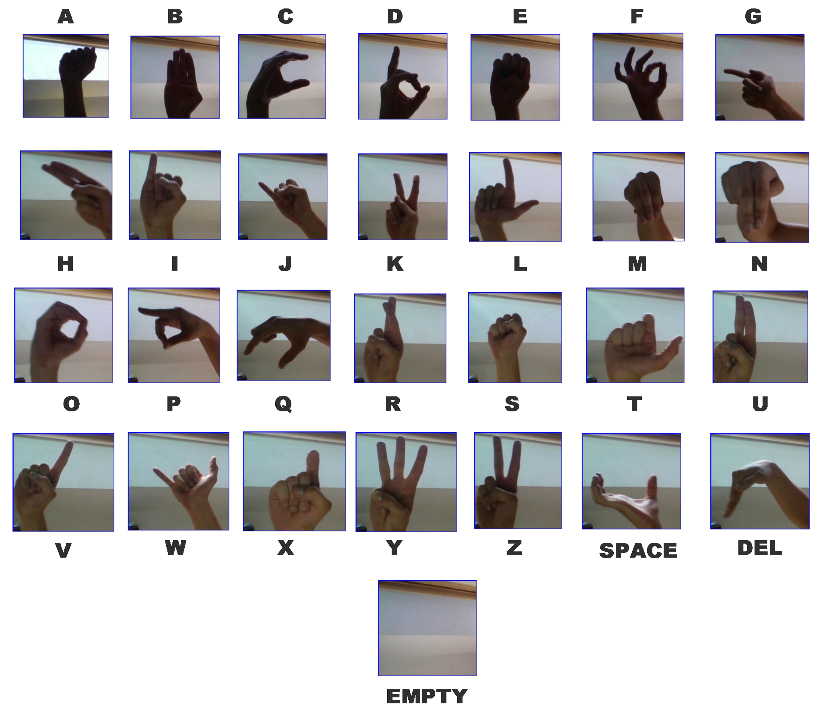
5. Dataset Description
6. Evaluation Metrics
7. Results
8. Comparison with Other Methodologies
9. Conclusions
Author Contributions
Funding
Conflicts of Interest
References
- Corballis, M.C. From mouth to hand: Gesture, speech, and the evolution of right-handedness. Behav. Brain Sci. 2003, 26, 199–208. [Google Scholar] [CrossRef] [PubMed]
- Liu, L.; Özsu, M.T. Encyclopedia of Database Systems; Springer: New York, NY, USA, 2009; Volume 6. [Google Scholar]
- LeCun, Y.; Denker, J.S.; Solla, S.A. Optimal Brain Damage. In Advances in Neural Information Processing Systems 8: Proceedings of the 1995 Conference; Morgan Kaufmann: San Francisco, CA, USA, 1990; pp. 598–605. [Google Scholar]
- He, K.; Zhang, X.; Ren, S.; Sun, J. Spatial pyramid pooling in deep convolutional networks for visual recognition. IEEE Trans. Pattern Anal. Mach. Intell. 2015, 37, 1904–1916. [Google Scholar] [CrossRef] [PubMed]
- Vogler, C.; Metaxas, D. Adapting hidden Markov models for ASL recognition by using three-dimensional computer vision methods. In Proceedings of the 1997 IEEE International Conference on Systems, Man, and Cybernetics, Computational Cybernetics and Simulation, Orlando, FL, USA, 12–15 October 1997; Volume 1, pp. 156–161. [Google Scholar]
- Vogler, C.; Metaxas, D. ASL recognition based on a coupling between HMMs and 3D motion analysis. In Proceedings of the Sixth International Conference on Computer Vision (IEEE Cat. No. 98CH36271), Bombay, India, 7 January 1998; pp. 363–369. [Google Scholar]
- Mitra, S.; Acharya, T. Gesture recognition: A survey. IEEE Trans. Syst. Man. Cybern. Part C 2007, 37, 311–324. [Google Scholar] [CrossRef]
- Hoshino, K.; Kawabuchi, I. A humanoid robotic hand performing the sign language motions. In Proceedings of the MHS2003 International Symposium on Micromechatronics and Human Science (IEEE Cat. No. 03TH8717), Nagoya, Japan, 19–22 October 2003; pp. 89–94. [Google Scholar]
- Karami, A.; Zanj, B.; Sarkaleh, A.K. Persian sign language (PSL) recognition using wavelet transform and neural networks. Expert Syst. Appl. 2011, 38, 2661–2667. [Google Scholar] [CrossRef]
- Weerasekera, C.S.; Jaward, M.H.; Kamrani, N. Robust asl fingerspelling recognition using local binary patterns and geometric features. In Proceedings of the 2013 International Conference on Digital Image Computing: Techniques and Applications (DICTA), Hobart, TAS, Australia, 26–28 November 2013; pp. 1–8. [Google Scholar]
- Bhuiyan, R.A.; Tushar, A.K.; Ashiquzzaman, A.; Shin, J.; Islam, M.R. Reduction of gesture feature dimension for improving the hand gesture recognition performance of numerical sign language. In Proceedings of the 2017 20th International Conference of Computer and Information Technology (ICCIT), Dhaka, Bangladesh, 22–24 December 2017; pp. 1–6. [Google Scholar]
- Oz, C.; Leu, M.C. American Sign Language word recognition with a sensory glove using artificial neural networks. Eng. Appl. Artif. Intell. 2011, 24, 1204–1213. [Google Scholar] [CrossRef]
- Vogler, C.; Metaxas, D. A framework for recognizing the simultaneous aspects of american sign language. Comput. Vis. Image Underst. 2001, 81, 358–384. [Google Scholar] [CrossRef]
- Ranga, V.; Yadav, N.; Garg, P. American sign language fingerspelling using hybrid discrete wavelet transform-gabor filter and convolutional neural network. J. Eng. Sci. Technol. 2018, 13, 2655–2669. [Google Scholar]
- Jung, R.; Kornhuber, H.; Da Fonseca, J.S. Multisensory Convergence on Cortical Neurons Neuronal Effects of Visual, Acoustic and Vestibular Stimuli in the Superior Convolutions of the Cat’s Cortex. Prog. Brain Res. 1963, 1, 207–240. [Google Scholar]
- LeCun, Y.; Bengio, Y. Convolutional networks for images, speech, and time series. Handb. Brain Theory Neural Netw. 1995, 3361, 1995. [Google Scholar]
- Krizhevsky, A.; Sutskever, I.; Hinton, G.E. Imagenet Classification with Deep Convolutional Neural Networks. Advances in Neural Information Processing Systems. 2012, pp. 1097–1105. Available online: http://www.cs.toronto.edu/~hinton/absps/imagenet.pdf (accessed on 19 August 2020).
- Kılıboz, N.Ç.; Güdükbay, U. A hand gesture recognition technique for human–computer interaction. J. Vis. Commun. Image Represent. 2015, 28, 97–104. [Google Scholar] [CrossRef]
- Kim, H.J.; Lee, J.S.; Park, J.H. Dynamic hand gesture recognition using a CNN model with 3D receptive fields. In Proceedings of the 2008 international conference on neural networks and signal processing, Nanjing, China, 7–11 June 2008; pp. 14–19. [Google Scholar]
- Lin, H.I.; Hsu, M.H.; Chen, W.K. Human hand gesture recognition using a convolution neural network. In Proceedings of the 2014 IEEE International Conference on Automation Science and Engineering (CASE), Taipei, Taiwan, 18–22 August 2014; pp. 1038–1043. [Google Scholar]
- Kim, S.Y.; Han, H.G.; Kim, J.W.; Lee, S.; Kim, T.W. A hand gesture recognition sensor using reflected impulses. IEEE Sens. J. 2017, 17, 2975–2976. [Google Scholar] [CrossRef]
- Zafrulla, Z.; Brashear, H.; Starner, T.; Hamilton, H.; Presti, P. American sign language recognition with the kinect. In Proceedings of the 13th International Conference on Multimodal Interfaces, Alicante, Spain, 14–18 November 2011; pp. 279–286. [Google Scholar]
- Ren, Z.; Yuan, J.; Meng, J.; Zhang, Z. Robust part-based hand gesture recognition using kinect sensor. IEEE Trans. Multimed. 2013, 15, 1110–1120. [Google Scholar] [CrossRef]
- Bantupalli, K.; Xie, Y. American sign language recognition using deep learning and computer vision. In Proceedings of the 2018 IEEE International Conference on Big Data (Big Data), Seattle, WA, USA, 10–13 December 2018; pp. 4896–4899. [Google Scholar]
- Tushar, A.K.; Ashiquzzaman, A.; Afrin, A.; Islam, M. A Novel Transfer Learning Approach upon Hindi, Arabic, and Bangla Numerals using Convolutional Neural Networks. arXiv 2017, arXiv:1707.08385. [Google Scholar]
- Islam, M.R.; Mitu, U.K.; Bhuiyan, R.A.; Shin, J. Hand gesture feature extraction using deep convolutional neural network for recognizing American sign language. In Proceedings of the 2018 4th International Conference on Frontiers of Signal Processing (ICFSP), Poitiers, France, 24–27 September 2018; pp. 115–119. [Google Scholar]
- Garcia, B.; Viesca, S.A. Real-time American sign language recognition with convolutional neural networks. Convolutional Neural Netw. Vis. Recognit. 2016, 2, 225–232. [Google Scholar]
- Akash. ASL Alphabet Dataset. 2018. Available online: https://www.kaggle.com/grassknoted/asl-alphabet (accessed on 19 August 2020).
- Goodfellow, I.; Bengio, Y.; Courville, A.; Bengio, Y. Deep Learning; MIT Press: Cambridge, UK, 2016; Volume 1. [Google Scholar]
- LeCun, Y.; Bengio, Y.; Hinton, G. Deep learning. Nature 2015, 521, 436–444. [Google Scholar] [CrossRef] [PubMed]
- LeCun, Y. The MNIST Database of Handwritten Digits. 1998. Available online: http://yann.lecun.com/exdb/mnist/ (accessed on 19 August 2020).
- Krizhevsky, A.; Hinton, G. Convolutional deep belief networks on cifar-10. 2010; unpublished manuscript. [Google Scholar]
- Sivic, J.; Zisserman, A. Video Google: A Text Retrieval Approach to Object Matching in Videos. In Proceedings of the IEEE International Conference on Computer Vision (ICCV 2003), Nice, France, 13–16 October 2003; p. 1470. [Google Scholar]
- Simonyan, K.; Zisserman, A. Very deep convolutional networks for large-scale image recognition. arXiv 2014, arXiv:1409.1556. [Google Scholar]
- Understanding the Backward Pass through Batch Normalization Layer. Available online: https://kratzert.github.io/2016/02/12/understanding-the-gradient-flow-through-the-batch-normalization-layer.html (accessed on 6 September 2017).
- Hu, H.; Peng, R.; Tai, Y.; Tang, C.; Trimming, N. A Data-Driven Neuron Pruning Approach towards Efficient Deep Architectures. arXiv 2016, arXiv:1607.03250. [Google Scholar]
- Clevert, D.A.; Unterthiner, T.; Hochreiter, S. Fast and accurate deep network learning by exponential linear units (elus). arXiv 2015, arXiv:1511.07289. [Google Scholar]
- Yue, J.; Mao, S.; Li, M. A deep learning framework for hyperspectral image classification using spatial pyramid pooling. Remote Sens. Lett. 2016, 7, 875–884. [Google Scholar] [CrossRef]
- Qu, T.; Zhang, Q.; Sun, S. Vehicle detection from high-resolution aerial images using spatial pyramid pooling-based deep convolutional neural networks. Multimed. Tools Appl. 2017, 76, 21651–21663. [Google Scholar] [CrossRef]
- Tushar, A.K.; Ashiquzzaman, A.; Islam, M.R. Faster convergence and reduction of overfitting in numerical hand sign recognition using DCNN. In Proceedings of the 2017 IEEE Region 10 Humanitarian Technology Conference (R10-HTC), Dhaka, Bangladesh, 21–23 December 2017; pp. 638–641. [Google Scholar]
- Chollet, F. Keras. 2015. Available online: https://github.com/fchollet/keras (accessed on 19 August 2020).
- Ioffe, S.; Szegedy, C. Batch normalization: Accelerating deep network training by reducing internal covariate shift. In Proceedings of the International Conference on Machine Learning, Lille, France, 7–9 July 2015; pp. 448–456. [Google Scholar]
- Ashiquzzaman, A.; Oh, S.; Lee, D.; Lee, J.; Kim, J. Compact Deeplearning Convolutional Neural Network based Hand Gesture Classifier Application for Smart Mobile Edge Computing. In Proceedings of the 2020 International Conference on Artificial Intelligence in Information and Communication (ICAIIC), Fukuoka, Japan, 19–21 Febuary 2020; pp. 119–123. [Google Scholar]


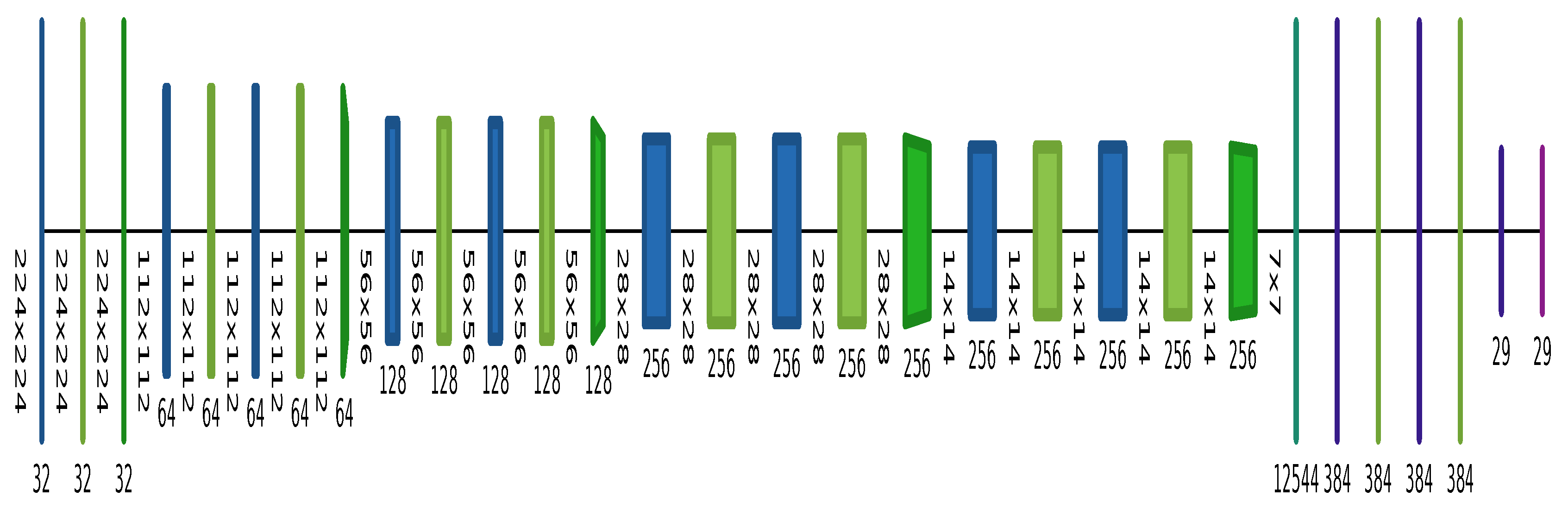
 ), batch normalization layers are lime (
 ) and max-pooling layers are forest green (
 ); these are followed by a flatten layer, shown in emerald green (
 ), a fully connected layer in violet (
 ) and the Softmax output in magenta (
 ). The number of dimensions in each layer is shown beside/below that layer.
), batch normalization layers are lime () and max-pooling layers are forest green (); these are followed by a flatten layer, shown in emerald green (), a fully connected layer in violet () and the Softmax output in magenta (). The number of dimensions in each layer is shown beside/below that layer.
). The number of dimensions in each layer is shown beside/below that layer.
), batch normalization layers are lime () and max-pooling layers are forest green (); these are followed by a flatten layer, shown in emerald green (), a fully connected layer in violet () and the Softmax output in magenta (). The number of dimensions in each layer is shown beside/below that layer. ), batch normalization layers are lime () and max-pooling layers are forest green (); these are followed by a flatten layer, shown in emerald green (), a fully connected layer in violet () and the Softmax output in magenta (). The number of dimensions in each layer is shown beside/below that layer.
), batch normalization layers are lime () and max-pooling layers are forest green (); these are followed by a flatten layer, shown in emerald green (), a fully connected layer in violet () and the Softmax output in magenta (). The number of dimensions in each layer is shown beside/below that layer.
), batch normalization layers are lime () and max-pooling layers are forest green (); these are followed by a flatten layer, shown in emerald green (), a fully connected layer in violet () and the Softmax output in magenta (). The number of dimensions in each layer is shown beside/below that layer.


| Original Deep Convolutional Network | Pruned Deep Convolutional Network | ||||
|---|---|---|---|---|---|
| Layers | Output Shape | Parameters | Layers | Output Shape | Parameters |
| Input | 224, 224, 3 | 0 | Input | 224, 224, 3 | 0 |
| (Conv2D) 64 | 224, 224, 64 | 1792 | (Conv2D) 32 | 224, 224, 32 | 896 |
| Batch Normalization | 224, 224, 64 | 256 | Batch Normalization | 224, 224, 32 | 128 |
| Max Pooling () | 112, 112, 64 | 0 | Max Pooling () | 112, 112, 32 | 0 |
| (Conv2D) 128 | 112, 112, 128 | 73,856 | (Conv2D) 64 | 112, 112, 64 | 18,496 |
| Batch Normalization | 112, 112, 128 | 512 | Batch Normalization | 112, 112, 64 | 256 |
| (Conv2D) 128 | 112, 112, 128 | 147,584 | (Conv2D) 64 | 112, 112, 64 | 36,928 |
| Batch Normalization | 112, 112, 128 | 512 | Batch Normalization | 112, 112, 64 | 256 |
| Max Pooling () | 56, 56, 128 | 0 | Max Pooling () | 56, 56, 64 | 0 |
| (Conv2D) 256 | 56, 56, 256 | 295,168 | (Conv2D) 128 | 56, 56, 128 | 73,856 |
| Batch Normalization | 56, 56, 256 | 1024 | Batch Normalization | 56, 56, 128 | 512 |
| (Conv2D) 256 | 56, 56, 256 | 590,080 | (Conv2D) 128 | 56, 56, 128 | 147,584 |
| Batch Normalization | 56, 56, 256 | 1024 | Batch Normalization | 56, 56, 128 | 512 |
| Max Pooling () | 56, 56, 256 | 0 | Max Pooling () | 28, 28, 128 | 0 |
| (Conv2D) 512 | 28, 28, 512 | 1,180,160 | (Conv2D) 256 | 28, 28, 256 | 295,168 |
| Batch Normalization | 28, 28, 512 | 2048 | Batch Normalization | 28, 28, 256 | 1024 |
| (Conv2D) 512 | 28, 28, 512 | 2,359,808 | (Conv2D) 256 | 28, 28, 256 | 590,080 |
| Batch Normalization | 28, 28, 512 | 2048 | Batch Normalization | 28, 28, 256 | 1024 |
| Max Pooling () | 14, 14, 512 | 0 | Max Pooling () | 14, 14, 256 | 0 |
| (Conv2D) 512 | 14, 14, 512 | 2,359,808 | (Conv2D) 256 | 14, 14, 256 | 590,080 |
| Batch Normalization | 14, 14, 512 | 2048 | Batch Normalization | 14, 14, 256 | 1024 |
| (Conv2D) 512 | 14, 14, 512 | 2,359,808 | (Conv2D) 256 | 14, 14, 256 | 590,080 |
| Batch Normalization | 14, 14, 512 | 2048 | Batch Normalization | 14, 14, 256 | 1024 |
| Max Pooling () | 7, 7, 512 | 0 | Max Pooling () | 7, 7, 256 | 0 |
| Flatten | 25,088 | 0 | Flatten | 12,544 | 0 |
| (Fully Connected) 512 | 512 | 12,845,568 | (Fully Connected) 384 | 384 | 4,817,280 |
| Batch Normalization | 512 | 2048 | Batch Normalization | 384 | 1536 |
| (Fully Connected) 512 | 512 | 262,656 | (Fully Connected) 384 | 384 | 147,840 |
| Batch Normalization | 512 | 2048 | Batch Normalization | 384 | 1536 |
| (Fully Connected) 512 | 29 | 14,877 | (Fully Connected) 29 | 29 | 11,165 |
| Output Softmax | 29 | 0 | Output Softmax | 29 | 0 |
| Total Parameters | 22,506,781 | Total Parameters | 7,328,285 | ||
| Layers | Output Shape | Parameters |
|---|---|---|
| Input | X, X, 3 | 0 |
| (Conv2D) 32 | X, X, 32 | 896 |
| Batch Normalization | X, X, 32 | 128 |
| Max Pooling () | X, X, 32 | 0 |
| (Conv2D) 64 | X, X,6 4 | 18,496 |
| Batch Normalization | X, X, 64 | 256 |
| (Conv2D) 64 | X, X, 64 | 36,928 |
| Batch Normalization | X, X, 64 | 256 |
| Max Pooling () | X, X, 64 | 0 |
| (Conv2D) 128 | X, X, 128 | 73,856 |
| Batch Normalization | X, X, 128 | 512 |
| (Conv2D) 128 | X, X, 128 | 147,584 |
| Batch Normalization | X, X, 128 | 512 |
| Max Pooling () | X, X, 128 | 0 |
| (Conv2D) 256 | X, X, 256 | 295,168 |
| Batch Normalization | X, X, 256 | 1024 |
| (Conv2D) 256 | X, X, 256 | 590,080 |
| Batch Normalization | X, X, 256 | 1024 |
| Max Pooling () | X, X, 256 | 0 |
| (Conv2D) 256 | X, X, 256 | 590,080 |
| Batch Normalization | X, X, 256 | 1024 |
| (Conv2D) 256 | X, X, 256 | 590,080 |
| Batch Normalization | X, X, 256 | 1024 |
| Max Pooling () | X, X, 256 | 0 |
| Spatial Pyramid Pooling | 5376 | 0 |
| (Fully Connected) 384 | 384 | 2,064,384 |
| Batch Normalization | 384 | 1536 |
| (Fully Connected) 384 | 384 | 147,840 |
| Batch Normalization | 384 | 1536 |
| (Fully Connected) 29 | 29 | 11,165 |
| Output Softmax | 29 | 0 |
| Total Parameters | 4,575,389 | |
| Total Data | Training Data | Testing Data |
|---|---|---|
| 87,000 | 69,600 | 17,400 |
| Layers | Numbers of Original Node/Filters | Numbers of Pruned Node/Filters | Percentage of Pruning | Worst Scored 20 Filters/Nodes |
|---|---|---|---|---|
| (Conv2D) 64 | 64 | 32 | 50 | 29, 7, 38, 31, 23, 54, 27, 40, 6, 42, 45, 61, 44, 25, 20, 15, 49, 4, 50, 1 |
| (Conv2D) 128 | 128 | 64 | 50 | 70, 39, 1, 64, 60, 110, 116, 119, 50, 84, 18, 107, 42, 89, 48, 15, 85, 7, 12, 58 |
| (Conv2D) 128 | 128 | 64 | 50 | 16, 49, 101, 100, 36, 88, 123, 91, 48, 97, 95, 78, 23, 55, 93, 68, 74, 108, 86, 82 |
| (Conv2D) 256 | 256 | 128 | 50 | 250, 82, 230, 186, 121, 62, 228, 35, 199, 64, 17, 133, 60, 143, 58, 57, 139, 31, 255, 135 |
| (Conv2D) 256 | 256 | 128 | 50 | 100, 88, 196, 245, 49, 118, 251, 170, 42, 138, 107, 92, 160, 238, 143, 199, 253, 191, 233, 36 |
| (Conv2D) 512 | 512 | 256 | 50 | 246, 273, 125, 166, 396, 287, 9, 233, 59, 111, 483, 22, 70, 423, 27, 370, 469, 232, 7, 372 |
| (Conv2D) 512 | 512 | 256 | 50 | 58, 119, 497, 221, 482, 487, 253, 251, 267, 160, 296, 204, 23, 179, 214, 278, 114, 48, 76, 414 |
| (Conv2D) 512 | 512 | 256 | 50 | 369, 454, 213, 317, 385, 395, 134, 147, 160, 346, 251, 58, 124, 360, 45, 205, 352, 445, 33, 498 |
| (Conv2D) 512 | 512 | 256 | 50 | 29, 79, 90, 313, 96, 27, 246, 436, 373, 298, 255, 148, 229, 262, 360, 9, 264, 150, 131, 172 |
| (Fully Connected) 512 | 512 | 384 | 25 | 251, 309, 244, 375, 218, 478, 153, 189, 146, 128, 357, 104, 325, 463, 430, 394, 253, 27, 441, 203 |
| (Fully Connected) 512 | 512 | 384 | 25 | 454, 98, 250, 410, 438, 124, 332, 175, 434, 297, 360, 5, 505, 436, 510, 69, 287, 32, 166, 504 |
| Original Model | Pruned Model | Convolutional Spatial Pyramid Pooling Model | ||||||||||
|---|---|---|---|---|---|---|---|---|---|---|---|---|
| Class | Precision | Recall | f1-Score | Support | Precision | Recall | f1-Score | Support | Precision | Recall | f1-Score | Support |
| 0 | 0.95 | 0.97 | 0.96 | 146 | 0.96 | 0.95 | 0.96 | 137 | 0.9 | 1 | 0.95 | 140 |
| 1 | 0.93 | 1 | 0.96 | 137 | 0.97 | 0.94 | 0.96 | 125 | 0.97 | 1 | 0.99 | 151 |
| 2 | 0.97 | 1 | 0.98 | 139 | 0.99 | 0.98 | 0.99 | 131 | 1 | 0.98 | 0.99 | 150 |
| 3 | 1 | 0.89 | 0.94 | 142 | 1 | 0.77 | 0.87 | 154 | 1 | 1 | 1 | 119 |
| 4 | 0.83 | 0.98 | 0.9 | 140 | 0.77 | 0.99 | 0.87 | 133 | 0.91 | 0.89 | 0.9 | 141 |
| 5 | 1 | 0.95 | 0.98 | 133 | 0.97 | 1 | 0.99 | 132 | 1 | 0.97 | 0.98 | 146 |
| 6 | 0.97 | 0.89 | 0.92 | 132 | 1 | 0.89 | 0.94 | 152 | 1 | 0.93 | 0.97 | 136 |
| 7 | 0.95 | 0.94 | 0.95 | 143 | 0.95 | 0.99 | 0.97 | 141 | 0.94 | 0.98 | 0.96 | 151 |
| 8 | 1 | 0.77 | 0.87 | 138 | 1 | 0.67 | 0.8 | 170 | 0.98 | 0.91 | 0.94 | 132 |
| 9 | 0.97 | 0.94 | 0.96 | 136 | 0.83 | 0.96 | 0.89 | 142 | 0.96 | 0.96 | 0.96 | 146 |
| 10 | 0.99 | 1 | 1 | 141 | 0.95 | 0.94 | 0.94 | 127 | 1 | 1 | 1 | 127 |
| 11 | 0.99 | 0.99 | 0.99 | 141 | 1 | 0.98 | 0.99 | 134 | 1 | 1 | 1 | 143 |
| 12 | 0.82 | 0.76 | 0.79 | 148 | 0.87 | 0.84 | 0.85 | 154 | 0.73 | 0.98 | 0.83 | 113 |
| 13 | 0.56 | 0.55 | 0.56 | 139 | 0.8 | 0.68 | 0.73 | 142 | 0.98 | 0.6 | 0.75 | 134 |
| 14 | 0.8 | 0.85 | 0.82 | 141 | 0.73 | 0.87 | 0.79 | 112 | 0.96 | 0.89 | 0.93 | 133 |
| 15 | 0.94 | 1 | 0.97 | 114 | 0.95 | 1 | 0.97 | 133 | 0.98 | 1 | 0.99 | 131 |
| 16 | 0.93 | 0.99 | 0.96 | 139 | 0.95 | 0.95 | 0.95 | 146 | 0.99 | 0.98 | 0.99 | 135 |
| 17 | 0.99 | 0.87 | 0.93 | 124 | 0.94 | 0.96 | 0.95 | 138 | 0.98 | 0.97 | 0.98 | 143 |
| 18 | 0.69 | 0.64 | 0.66 | 135 | 0.66 | 0.97 | 0.78 | 132 | 0.68 | 0.94 | 0.79 | 144 |
| 19 | 0.95 | 0.75 | 0.84 | 129 | 0.97 | 0.81 | 0.89 | 143 | 0.89 | 0.96 | 0.92 | 140 |
| 20 | 0.78 | 0.99 | 0.88 | 143 | 0.88 | 0.91 | 0.89 | 144 | 1 | 0.97 | 0.98 | 150 |
| 21 | 0.88 | 0.99 | 0.93 | 137 | 0.92 | 0.98 | 0.95 | 126 | 0.98 | 0.99 | 0.99 | 128 |
| 22 | 0.84 | 0.95 | 0.89 | 140 | 0.83 | 0.99 | 0.91 | 130 | 0.95 | 1 | 0.97 | 124 |
| 23 | 0.7 | 0.57 | 0.63 | 128 | 0.99 | 0.6 | 0.75 | 142 | 0.97 | 0.44 | 0.6 | 133 |
| 24 | 0.87 | 0.91 | 0.89 | 137 | 0.92 | 0.92 | 0.92 | 130 | 0.96 | 0.9 | 0.93 | 144 |
| 25 | 0.88 | 0.97 | 0.92 | 144 | 0.94 | 0.97 | 0.95 | 118 | 0.85 | 1 | 0.92 | 144 |
| 26 | 0.96 | 0.91 | 0.93 | 148 | 0.95 | 0.95 | 0.95 | 153 | 0.99 | 0.99 | 0.99 | 140 |
| 27 | 1 | 0.99 | 0.99 | 144 | 0.9 | 0.98 | 0.93 | 131 | 0.92 | 1 | 0.96 | 142 |
| 28 | 0.99 | 1 | 1 | 142 | 0.97 | 1 | 0.98 | 148 | 1 | 1 | 1 | 140 |
| accuracy | - | - | 0.9 | 4000 | - | - | 0.91 | 4000 | - | - | 0.94 | 4000 |
| macro avg. | 0.9 | 0.9 | 0.9 | 4000 | 0.92 | 0.91 | 0.91 | 4000 | 0.95 | 0.94 | 0.94 | 4000 |
| weighted avg. | 0.9 | 0.9 | 0.9 | 4000 | 0.92 | 0.91 | 0.91 | 4000 | 0.95 | 0.94 | 0.94 | 4000 |
| Original Parameters | After Pruned | Pruned Parameters |
|---|---|---|
| 22,498,973 | 7,323,869 | 15,175,104 |
| Total Compression (%) | 67.45% |
| Original Model | Pruned Model | Spatial Pyramid Pooling Model | |||
|---|---|---|---|---|---|
| Accuracy | -Score | Accuracy | -Score | Accuracy | -Score |
| 90.9761 | 0.9050 | 91.7250 | 0.9262 | 93.1249 | 0.9415 |
| 90.9762 | 0.9022 | 91.3250 | 0.9206 | 94.3750 | 0.9599 |
| 90.9761 | 0.9125 | 91.2750 | 0.9392 | 93.8000 | 0.9384 |
| 90.9761 | 0.9227 | 92.6429 | 0.9206 | 93.3571 | 0.9487 |
| 90.5814 | 0.9148 | 89.1129 | 0.9241 | 93.1500 | 0.9552 |
| Model Name | Run Time (s) | Comment |
|---|---|---|
| Modified VGG-like Proposed Model | 19.30 ± 1.32 | - |
| Proposed Pruned Model | 9.34 ± 1.37 | - |
| Spatial Pyramid Pooling Model | 4.10 ± 8.97 | - |
| Spatial Pyramid Pooling Model | 0.013 ± 0.019 | (Multi-GPU) |
| Total Class in Sequence | Run Time (ms) |
|---|---|
| 3 | 136 ± 1.98 |
| 4 | 173 ± 3.36 |
| 5 | 202 ± 8.97 |
| 6 | 267 ± 2.13 |
| Image Samples in Each Class (fps) | Original Generated Sequence | Pruned Classifier Predicted Sequence | Mean Majority in Rows (Percent) | Spatial Pyramid Classifier Predicted Sequence | Mean Majority in Rows (Percent) |
|---|---|---|---|---|---|
| 5 | [‘H’ ‘K’ ‘J’ ‘M’] | [‘H’ ‘K’ ‘J’ ‘M’] | 99.20 | [‘H’ ‘K’ ‘J’ ‘M’] | 100 |
| [‘Y’ ‘G’ ‘Z’ ‘X’] | [‘Y’ ‘G’ ‘Z’ ‘X’] | 99.20 | [‘Y’ ‘G’ ‘Z’ ‘X’] | 100 | |
| [‘T’ ‘C’ ‘W’ ‘V’] | [‘T’ ‘C’ ‘W’ ‘V’] | 99.20 | [‘T’ ‘C’ ‘W’ ‘V’] | 100 | |
| 10 | [‘H’ ‘K’ ‘J’ ‘M’] | [‘H’ ‘K’ ‘J’ ‘M’] | 99.23 | [‘H’ ‘K’ ‘J’ ‘M’] | 100 |
| [‘Y’ ‘G’ ‘Z’ ‘X’] | [‘Y’ ‘G’ ‘Z’ ‘X’] | 98.2 | [‘Y’ ‘G’ ‘Z’ ‘X’] | 100 | |
| [‘T’ ‘C’ ‘W’ ‘V’] | [‘T’ ‘C’ ‘W’ ‘V’] | 98.2 | [‘T’ ‘C’ ‘W’ ‘V’] | 99.97 | |
| 30 | [‘H’ ‘K’ ‘J’ ‘M’] | [‘H’ ‘K’ ‘J’ ‘M’] | 99.23 | [‘H’ ‘K’ ‘J’ ‘M’] | 99.88 |
| [‘Y’ ‘G’ ‘Z’ ‘X’] | [‘Y’ ‘G’ ‘Z’ ‘X’] | 98.99 | [‘Y’ ‘G’ ‘Z’ ‘X’] | 99.3 | |
| [‘T’ ‘C’ ‘W’ ‘V’] | [‘T’ ‘C’ ‘W’ ‘V’] | 98.99 | [‘T’ ‘C’ ‘W’ ‘V’] | 99.33 | |
| 60 | [‘H’ ‘K’ ‘J’ ‘M’] | [‘H’ ‘K’ ‘J’ ‘M’] | 98.99 | [‘H’ ‘K’ ‘J’ ‘M’] | 99.33 |
| [‘Y’ ‘G’ ‘Z’ ‘X’] | [‘Y’ ‘G’ ‘Z’ ‘X’] | 98.24 | [‘Y’ ‘G’ ‘Z’ ‘X’] | 99.67 | |
| [‘T’ ‘C’ ‘W’ ‘V’] | [‘T’ ‘C’ ‘W’ ‘V’] | 98.56 | [‘T’ ‘C’ ‘W’ ‘V’] | 99.33 |
Publisher’s Note: MDPI stays neutral with regard to jurisdictional claims in published maps and institutional affiliations. |
© 2020 by the authors. Licensee MDPI, Basel, Switzerland. This article is an open access article distributed under the terms and conditions of the Creative Commons Attribution (CC BY) license (http://creativecommons.org/licenses/by/4.0/).
Share and Cite
Ashiquzzaman, A.; Lee, H.; Kim, K.; Kim, H.-Y.; Park, J.; Kim, J. Compact Spatial Pyramid Pooling Deep Convolutional Neural Network Based Hand Gestures Decoder. Appl. Sci. 2020, 10, 7898. https://doi.org/10.3390/app10217898
Ashiquzzaman A, Lee H, Kim K, Kim H-Y, Park J, Kim J. Compact Spatial Pyramid Pooling Deep Convolutional Neural Network Based Hand Gestures Decoder. Applied Sciences. 2020; 10(21):7898. https://doi.org/10.3390/app10217898
Chicago/Turabian StyleAshiquzzaman, Akm, Hyunmin Lee, Kwangki Kim, Hye-Young Kim, Jaehyung Park, and Jinsul Kim. 2020. "Compact Spatial Pyramid Pooling Deep Convolutional Neural Network Based Hand Gestures Decoder" Applied Sciences 10, no. 21: 7898. https://doi.org/10.3390/app10217898
APA StyleAshiquzzaman, A., Lee, H., Kim, K., Kim, H.-Y., Park, J., & Kim, J. (2020). Compact Spatial Pyramid Pooling Deep Convolutional Neural Network Based Hand Gestures Decoder. Applied Sciences, 10(21), 7898. https://doi.org/10.3390/app10217898