Deep Neural Network-Based Guidance Law Using Supervised Learning

Abstract

This paper proposes that the deep neural network-based guidance (DNNG) law replace the proportional navigation guidance (PNG) law. This approach is performed by adopting a supervised learning (SL) method using a large amount of simulation data from the missile system with PNG. Then, the proposed DNNG is compared with the PNG, and its performance is evaluated via the hitting rate and the energy function. In addition, the DNN-based only line-of-sight (LOS) rate input guidance (DNNLG) law, in which only the LOS rate is an input variable, is introduced and compared with the PN and DNNG laws. Then, the DNNG and DNNLG laws examine behavior in an initial position other than the training data.

1. Introduction

Proportional navigation guidance (PNG) is one of the most widely known missile guidance laws in existence [1]. This guidance law generates an acceleration command proportional to the line-of-sight (LOS) rate from the perspective of a missile looking at a target. This is easy to implement based on simple principles.

Raj [2] demonstrated the performance of PNG by showing that PNG is effective in intercepting a low-maneuvering target in a two-dimensional missile target engagement scenario. Bryson and Ho [3] showed that PNG is the optimal solution for engagement scenarios for a missile with constant speed and a stationary target by solving linearized engagement equations. This guidance law enables various designs according to the navigation constants with arbitrary real number values. Based on the fact that the form or size of the guidance command varies depending on the navigation constants, Yang [4] proposed a recursive optimal pure proportional navigation (PPN) scheme that predicts recursively optimal navigation gain and time-to-go. It also showed that the proposed algorithm applies to maneuvering targets. Kim [5] proposed a robust PNG law, a form of combination of the conventional PNG and the switching part made by using the Lyapunov approach. This was robust when used against a highly maneuvering target.

Recently, deep learning [6]-based artificial intelligence technology has received attention in academia and industry. Various studies using artificial neural networks (ANNs) are also being studied in the defense technology sector, and among them, guidance laws have become the focus of various research as they are essential in homing missiles [7,8,9,10,11,12,13]. Balakrishnan and Biega [7] presented a new neural structure providing feedback guidance solutions for any initial conditions and time-to-go for two-dimensional scenarios. Lee et al. [8,9] proposed a neural network guidance algorithm for bank-to-turn (BTT) missiles. This guidance performance was verified by comparing it with PNG. Rahbar and Bahrami [10] presented a method of designing a feedback controller of homing missile using feed-forward multi-layer perceptron (MLP). They demonstrated the efficiency of the proposed method by performing simulations on various initial input values. Rajagopalan et al. [14] presented an ANN-based approach using MLP to replace PNG. It showed that MLP-based guidance can effectively replace the PNG in a wide range of engagement scenarios.

In this paper, we propose a deep neural network-based guidance (DNNG) law imitating PNG. This approach learns the DNN model with training data acquired from PNG. The DNN model applies to the missile system instead of PNG, and its performance is comparable with PNG. Then, we design the controller model and discuss how the proposed DNNG law changes according to time constants.

This paper is organized as follows: In Section 2, the two-dimensional missile–target engagement scenario and equations of motion of the missile will be explained. Section 3 briefly describes the conventional PNG law. In Section 4, the DNNG law that applied supervised learning, such as training data collection, DNNG structure, training methods and evaluation, is described in detail. Additionally, the simulation results of the DNNG law are shown through numerical simulation. Section 5 introduces a new DNN-based guidance law with the input variables of only the LOS rates. We run simulations at the initial position outside the range of training data. In addition, we design the first-order system and examine the energy performance of the missile according to the time constant. Finally, conclusions are given in Section 6.

2. Problem Statement

2.1. Equations of Motion

The missile is attempting to hit the stationary target. The missile has a constant speed and hits the target by controlling the lateral acceleration command. Figure 1 shows the two-dimensional engagement geometry between the missile and the target.

Figure 1. Two-dimensional engagement geometry.

Here, $R$ is the relative distance from the missile to the target, $V_m$ is the speed of the missile, $a_m$ is the lateral acceleration command of the missile, $\lambda$ is the look angle, ${\psi }_m$ is the heading angle of the missile and $\mathsf{\Omega }$ is the LOS rate. Let us define the LOS angle ($\sigma$) as a contained angle formed between the look angle and the heading angle. The motion of the missile is expressed via nonlinear differential equations, such as Equations (1)–(4).

$$\dot{R}=- V_m\cos \left(\lambda -{\psi }_m\right)$$

(1)

$$\dot{\lambda }=\frac{V_m}{R}sin\left(\lambda -{\psi }_m\right)$$

(2)

$${\dot{\psi }}_m=\frac{a_m}{V_m}$$

(3)

$$\sigma =\lambda -{\psi }_m$$

(4)

The allowable range of lateral acceleration of the missile is set as follows:

$$-10g\le a_m\le 10g$$

(5)

where the acceleration of gravity is $g=9.81 \mathrm{m}/{\mathrm{s}}^2$. This paper addresses the engagement scenario between the anti-ship missile and the target. It is assumed that the missile flies at a constant speed between Mach 0.5 and 0.95, and that the target is stationary.

2.2. Engagement Scenario

The assumptions of the engagement scenarios of this paper are as follows: First, the initial position of the missile starts at any position $\mathrm{20,000}~ \mathrm{30,000} \left(\mathrm{m}\right)$ away from the target. Second, the initial heading angle of the missile is any values between $-\frac{\pi }{2}$ and $\frac{\pi }{2} \left(\mathrm{rad}\right)$, centered on the look angle of the missile. Third, the missile is regarded as having hit the target if the relative distance between the missile and the target is within $2\mathrm{m}.$ Finally, the target is stationary in position $\left(x_t, y_t\right)=\left(0, 0\right)$.

$\theta$ in Figure 2 and Table 1 represent the angle of the missile viewed by the target in the polar coordinate system. In Figure 2, the positive x-axis direction is $0, 2\pi \left(\mathrm{rad}\right)$, measured counter-clockwise to indicate the magnitude of that angle.

Figure 2. Missile–target engagement scenario.

Table 1. Initial conditions of the missile.

${\mathit{R}}_0 \left(\mathbf{m}\right)$	${\mathit{\theta }}_0 \left(\mathbf{r}\mathbf{a}\mathbf{d}\right)$	${\mathit{\lambda }}_0 \left(\mathbf{r}\mathbf{a}\mathbf{d}\right)$	${\mathit{\psi }}_0 \left(\mathbf{r}\mathbf{a}\mathbf{d}\right)$	${\mathit{V}}_{\mathit{m}} \left(\mathbf{m}/\mathbf{s}\right)$
$\left[ 20,000,30,000 \right]$	$\left[ 0, 2\pi \right]$	$\left[ \theta +\pi \right]$	$\left[ {\lambda }_0-\frac{\pi }{2}, {\lambda }_0+\frac{\pi }{2} \right]$	$\left[ 170,323 \right]$

The initial conditions of the missile are shown in Table 1. The initial values of the missile have random values within the presented range, and the simulation is terminated if the final distance of $2\mathrm{m}$ is satisfied.

3. Proportional Navigation Guidance Law

The proportional navigation guidance (PNG) law is used on almost all homing missiles. Recently, it has actively used methods to improve the performances of missiles using modern control theory, but this is basically an extension of the PNG. PNG is based on the principle that the missile’s acceleration is generated in proportion to the LOS rate of the target if the LOS is constant when the two objects approach each other. Since the LOS rate is measured by the seeker of the missile, the performance of the seeker has a significant effect on the missile’s motion trajectory.

In addition, PNG is very useful for missile guidance problems against stationary targets. The characteristic of this guidance law is that if the acceleration is generated such that the LOS rate is zero, it can hit the target without any special maneuvering of the missile. Moreover, the same principle could be applied to moving targets. Figure 3 shows the form of the guidance geometry of the impact triangle, which ensures the look angle is parallel to the moving target. In other words, in order to apply this guidance law, the missile’s seeker requires two pieces of information: the speed and LOS rate of the missile. The form of the PNG is as follows:

$$a_m=N{V}_m\mathsf{\Omega }$$

(6)

where $N$ is navigation constant, $V_m$ is the speed of the missile and $\mathsf{\Omega }$ is LOS rate.

Figure 3. Conceptual diagram of proportional navigation guidance.

4. DNN-Based Guidance (DNNG) Law

In this section, we explain the DNN-based guidance (DNNG) law, which begins with the acquisition of training data from missile systems with the PNG law. The DNNG law is a deep neural network that deduces one output variable for two input variables, and has the same principle as the PNG law. This law outputs an acceleration, $a_m$, by inputting the LOS rate, $\mathsf{\Omega }$, and the speed of the missile, $V_m$. Figure 4 shows a schematic diagram for the approach of this paper, indicating that the DNNG replaces the PNG. This missile system consists of three main modules: the seeker module, the guidance module and the dynamics module. The seeker module identifies the target position, and then this outputs the LOS rate and the speed of the missile. The guidance module then generates the acceleration commands for the missile in accordance with the guidance law. The dynamics module calculates the state of the missile through numerical integration based on the missile dynamics using control values.

Figure 4. Schematic diagram of the missile system.

Figure 5 shows the process of supervised learning for the DNNG. The learning process consists of a collection of the training data, the DNN architecture design and optimization. The details of the learning process are covered in the following paragraph. The performance evaluation of DNNG is carried out in the missile system simulator established in this study, and its performance is compared with the PNG.

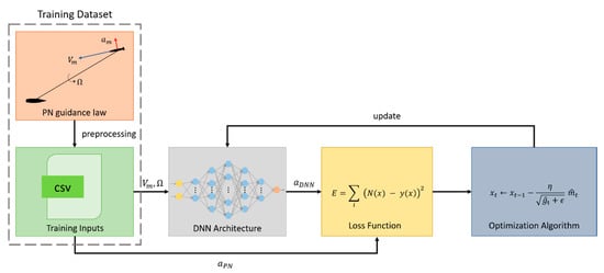
Figure 5. Learning process of supervised learning.

4.1. Data Collection

The dataset used for supervised learning (SL) is generated from the simulation data of the missile system with PNG for the missile–target engagement scenario. This missile system with PNG was constructed with MATLAB/Simulink. The DNNG model is trained to learn about the relationship between state and action from the PNG-based generated dataset. The dataset consists of $\left(x^{*}, u^{*}\right)$ pairs, the state variables $x^{*}$ are the LOS rate $\mathsf{\Omega }$ and the speed of the missile $V_m$, and the action variable $u^{*}$ is the lateral acceleration of the missile $a_m$. The state–action pairs are clean data without considering noise. The purpose is to create a DNN-based guidance law using information received from the seeker. Two pieces of information are provided from the seeker: the LOS rate and the speed of the missile. The initial conditions used for data collection were randomly generated within the bounds shown in Table 1. That is, the initialization area $A$ is defined as $x_0\in A$, which is an area that contains all the values within the initial bounds in Table 1. The training data consisted of a total of $89,025$ trajectories and $1,108,587,789$ state–control pairs, which were sampled at 0.01 s intervals. Figure 6 shows the initial position distribution of the missile. It appears that its position is uniformly distributed. In addition, the initial heading angle of the missile is uniformly distributed within the range $-\frac{\pi }{2}$~$\frac{\pi }{2}$, based on the look angle. This shows that the training data used to learn the DNN model are trained in various initial conditions, and that at the same time the initial conditions have a sufficiently uniform distribution. The constant value used for learning the DNNG is as follows: the navigation constant $N$ is 3, and the speed of the missile $V_m$ has an arbitrary value between Mach $0.5$ and $0.95$, respectively.

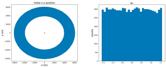
Figure 6. Distribution of the initial position and heading angle of the training dataset.

4.2. DNNG Architecture

The DNNG architecture consists of a fully connected layer. The output for each layer can be expressed mathematically, and the output of the i-th layer can be represented as shown in Equation (7).

$$o_i=a_i\left(W_i{o}_{i-1}+b_i\right)$$

(7)

where $a_i$ is the activation function, $W_i$ are the weighting vectors, $o_{i-1}$ is the output of the previous layer, $b_i$ is bias and $i$ is the number of hidden layers.

The selection of an activation function is very important in designing a DNN model. In this study, we experimented with various activation functions, and among them, the DNN model consisting of only a hyperbolic tangent function had the best performance. Thus, in this study, the activation function selects a hyperbolic tangent function as defined in Equation (8), which applies for both the output and hidden layers.

$$\tanh \left(x\right)=\frac{e^x-e^{-x}}{e^x+e^{-x}} \left(x=W_i{o}_{i-1}+b_i\right)$$

(8)

4.3. Training

In order to obtain the optimal value of the weight parameter from the training data at the training stage, whenever the training process is repeated, the loss function for the DNNG-driven actions and the PNG-driven actions tries to minimize the loss. Each iteration was evaluated using the mean squared error (MSE) loss function for the difference between the PNG-driven action, $a_{PN}$, and the DNNG-driven action, $a_{DNN}$, as defined in Equation (9).

$$Loss=\frac{1}{2} {\displaystyle \sum }_i {\left(a_{DNN}- a_{PN}\right)}^2$$

(9)

The DNNG model has been trained using an adaptive moment estimation (Adam) optimizer. The Adam optimization algorithm is not affected by the rescaling of the gradient. Therefore, regardless of the size of the gradient, since the step size is bound, it will be a stable gradient descent. This feature is considered an appropriate optimization algorithm to solve this problem. Here, hyper parameters use the default value of the python class of Adam optimization, and these are ${\mathsf{\beta }}_1\approx 0.9$, $\beta \approx 0.999$, $ϵ\approx {10}^{-8}$ and $\eta =0.0001$, respectively [15].

4.4. Evaluation

The action can be derived through the DNNG model for any state, and the mean absolute error (MAE) can evaluate the difference between the accelerations derived from the DNNG and from the PNG. The MAE is represented in Equation (10).

$$\left|a_{DNN}- a_{PN}\right|$$

(10)

This measurement can only evaluate the performance of the DNNG model, but how the DNNG law works in the missile environment cannot be known exactly. A small error in generating the trajectory from system dynamics may be enough to result in a failure to hit the target. Thus, we need an additional evaluation for the DNNG law. The additional evaluation is performed by replacing the PNG law of the missile simulator with the DNNG law. We find the DNNG-driven trajectory through the numerical integration of missile system dynamics, such as in Equation (11).

$$x\left(t\right)={{\displaystyle \int }}_0^{t_f}f\left(x\left(t\right), DNN\left(x\left(t\right)\right)\right)dt$$

(11)

Comparing the trajectories of missiles is a useful method to compare the DNNG and PNG laws. Moreover, the energy of the missile used at this time is an important criterion to confirm the performance of the missile guidance law. Therefore, the energy equation of the missile is defined as follows in Equation (12):

$$Energy={{\displaystyle \int }}_0^{t_f}{a}_m^{2}dt$$

(12)

The total energy required for a missile flight is an important measure of whether the missile trajectory is optimized or not. The simulation results will show how well the DNNG law has been learned from the PNG law through energy performance.

4.5. Simulation Results

This section shows the simulation results of the DNNG law for various initial conditions. The simulation was performed on clean data without considering noise. The energy performance of the DNNG law was evaluated for 100 random initial conditions. The simulation was performed with an integration step of 0.01 s. In addition, DNNG is compared not only with PNG, but also with the reinforcement learning-based guidance (RLG) law presented in the previous paper [16], and this demonstrates its performance through the energy term. Table 2 shows the average value of the simulation of three missile guidance laws for 100 random initial conditions. Here, $t_f$ is the final time, $R_f$ is the final distance and the energy is the value calculated using Equation (12). The DNNG law derives almost the same results as the PNG, although very small errors can occur in numerical calculations. The simulation results show that DNNG uses less energy than RL-based guidance, and is implied to have a sufficient performance to replace PNG.

Table 2. Performance comparison of three guidance laws for 100 random initial conditions.

Guidance Law	${\mathit{t}}_{\mathit{f}} \left(\mathit{s}\right)$	${\mathit{R}}_{\mathit{f}} \left(\mathit{m}\right)$	Energy
PNG	$117.2338$	$0.7323$	$1507.7367$
DNNG	$116.2438$	$0.6440$	$1507.7142$
RLG [16]	113.0026	0.9789	1670.2785

Figure 7 and Figure 8 shows the acceleration and the trajectory of the missile, respectively. The initial conditions are as follows: $R_0=\mathrm{28,516} \left(\mathrm{m}\right), {\lambda }_0=4.0915 \left(\mathrm{rad}\right), {\psi }_0=5.1782 \left(\mathrm{rad}\right), V_m=230 \left(\mathrm{m}/\mathrm{s}\right)$. The simulations of the DNNG and PNG laws show almost the same result. The final distance and the energy performance of the PNG law are $1.1356 \mathrm{m}$ and $1302.3000$, and those of the DNNG law are $0.2785 \mathrm{m}$ and $1302.3153$, respectively. Both guidance laws were successful in hitting the target by entering the $2\mathrm{m}$ margin. The simulation result suggests that the DNNG law is able to replace the PNG law.

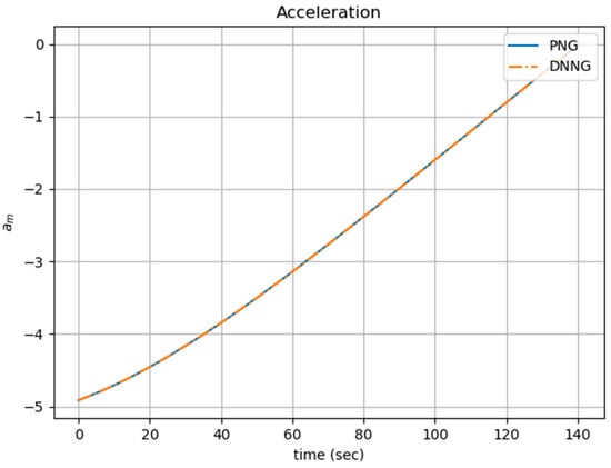
Figure 7. Comparison of the acceleration of PNG and DNNG laws.

Figure 8. Comparison of the trajectory of PNG and DNNG laws.

5. Results

In this section, we show the additional experiments for the DNNG law. The following three experiments were performed. The first experiment was to subtract the speed information from the input variables of the DNNG module. In other words, this will show the behavior of the missile when there is only one input variable of the DNNG law, the LOS rate. The second examines the behavior of the missile in its initial position not used in the DNN learning. The last interprets the guidance and control loops for all guidance laws.

5.1. Additional Experiment

In this section, we assess the behavior of the DNNG-driven trajectory when the input variables of the guidance module are reduced to one. This is called the DNN-based only LOS rate input guidance (DNNLG) law because there is only one input variable entering the guidance loop. The DNNLG law learns state–action relationships using state variable $\mathsf{\Omega }$ and action variable $a_m$ from the training data generated by the PNG law. Figure 9 shows the schematic diagram of the missile system with the DNNLG law and the guidance law operates with only the LOS rate.

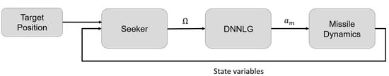
Figure 9. Missile system with DNNLG law.

The data collection, DNNG architecture, DNNG training and evaluation to create DNNLG are carried out via the same method as in Section 4. Figure 10 and Figure 11 show the simulation results for three guidance laws. The initial conditions are as follows: $R_0=\mathrm{26,252} \left(\mathrm{m}\right), {\lambda }_0=0.5564 \left(\mathrm{rad}\right), {\psi }_0=-0.2497 \left(\mathrm{rad}\right), V_m=268 \left(\mathrm{m}/\mathrm{s}\right)$ The energy values of the missile for PNG, DNNG and DNNLG are $3.0942, 3.0935$ and $3.4034$, respectively.

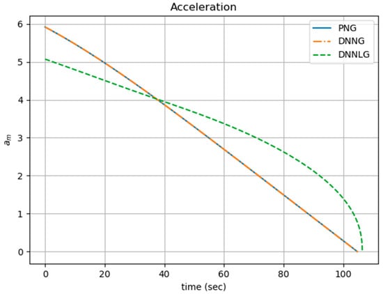
Figure 10. Comparison of the acceleration for all guidance law.

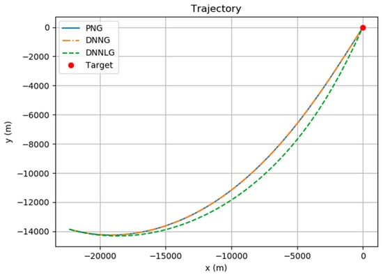
Figure 11. Comparison of the trajectory for all guidance law.

The average values of the DNNLG were obtained using 100 random items from the validation data in Section 4. These results are given in Table 3. Comparing Table 2 to Table 3, DNNG produces simulation results that are roughly the same as PNG, but DNNLG shows inferior performance to the other two guidance systems in terms of optimality. However, in terms of hitting the targets, DNNLG indicates that it can be used to replace PNG. This experiment tells us that the missile can maneuver while only knowing the minimum input variable, the value for the LOS rate.

Table 3. Results of DNNLG law for 100 random initial conditions.

Guidance Law	$t_f \left(s\right)$	$R_f \left(m\right)$	Energy
DNNLG	$117.0477$	$0.5424$	$1568.9078$

This simulation result shows the limitation of SL. SL produces completely identical results for complete input–output pairs, however, changing the input–output variables results in a difference from the training data. Therefore, it is very important to construct training data in supervised learning.

5.2. Initial Conditions Outside of the Learning Range

This study examined how DNNG works in an untrained initial position. We assumed that the missile departs from a position that is less than $\mathrm{20,000}$ $m$ and greater than $\mathrm{30,000}$ $\mathrm{m}$ from away the position used in the learning ($20,000~30,000 \mathrm{m}$). All guidance is simulated from 100 arbitrary random validation data. The hit rate and the energy average for the 100 random initial conditions are shown in Table 4. In Table 4, all guidance laws satisfy the accuracy of $2 \mathrm{m}$.

Table 4. Average energy for the 100 random initial conditions outside the range of the training data.

Guidance Law	Hit Rate (%)	Energy
PNG	$100$	$1195.4409$
DNNG	$100$	$1195.6002$
DNNLG	$100$	$1252.1283$
RLG [16]	100	$1287.4488$

The simulation results show that DNNG can be used for any initial position. In addition, the DNNG model shows that the training data pairs of the PNG are well learned. In other words, it suggests that DNNG is enough to replace PNG. On the other hand, DNNLG results in a slightly different maneuver from the PNG because this has not completely learned the state–control pairs of the PNG.

5.3. Design of the Controller Model

A controller model is designed for the control of the acceleration of a missile. The practical system model is expressed with a high-order system, but this study is defined as a first-order system with a time constant $\tau$ for simple analysis. The first-order control system can be expressed mathematically with a first-order differential equation, and the characteristic of the transient response relies entirely on the time constant $\tau$. Thus, acceleration commands which are intended to be controlled can be represented by the first-order system, such as in Equation (13). The system response is determined by the time constant $\tau$.

$$\tau {\dot{a}}_m+a_m=a_{cmd}$$

(13)

where $\tau$ is the time constant, $a_m$ is the derived acceleration and $a_{cmd}$ is the acceleration command.

Figure 12 shows a schematic diagram of the missile simulator with a first-order system. The first-order system can be viewed as a linear time-invariant (LTI) input–output system. The missile is maneuvered by acceleration derived from the controller model. Thus, the trajectory simulation is executed with acceleration commands that have passed through the first-order system.

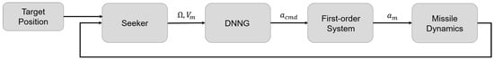
Figure 12. Conceptual diagram of the missile system with added first-order system.

The DNNG and DNNLG laws are trained without a controller model. These two guidance laws are trained as a state–control pair of the PNG with a navigation constant of 3. The simulation is performed for the time constant $\left\{0, 0.05, 0.07, 0.1, 0.5, 1\right\}$ on 150 random initial conditions. The simulation results are shown in Table 5. The DNNG and DNNLG laws have a 100% hit rate under all initial conditions. The DNNG makes a difference from the PNG as the time constant grows, which appears to be the result of training without considering the controller model during the DNNG model’s training. Thus, SL cannot achieve the same results entirely for the data other than the training data, while fully learning about training data. These results seem to reveal the limit of SL, and to make up for it, we need to explore other ways, such as building a very large database that takes into account all the factors, or using reinforcement learning (RL).

Table 5. Hit rate and average energy of the three different guidance laws for 150 random initial conditions according to time constant.

Time Constant	Guidance	Hit Rate (%)	Energy
$0$	PNG	$100$	$1061.5301$
	DNNG	$100$	$1061.5235$
	DNNLG	$100$	$1108.8668$
$0.05$	PNG	$100$	$1061.7394$
	DNNG	$100$	$1062.4931$
	DNNLG	$100$	$1109.1051$
$0.07$	PNG	$100$	$1061.8672$
	DNNG	$100$	$1062.6036$
	DNNLG	$100$	$1109.1523$
$0.1$	PNG	$100$	$1062.0621$
	DNNG	$100$	$1062.7446$
	DNNLG	$100$	$1109.2414$
$0.5$	PNG	$100$	$1064.7169$
	DNNG	$100$	$1065.1657$
	DNNLG	$100$	$1110.9848$
$1$	PNG	$100$	$1068.1829$
	DNNG	$100$	$1068.5402$
	DNNLG	$100$	$1113.7670$

6. Conclusions

In this paper, we proposed that DNNG can replace conventional PNG. The proposed guidance law was simulated in a two-dimensional missile–target engagement scenario. DNNG completely imitated PNG, and this was enough to replace PNG. Additionally, three experimental results were obtained regarding DNNG’s abilities. Firstly, we introduced DNNLG such that only the LOS rate was the input variable. DNNLG had a hit rate of 100%, but this guidance law did not fully follow PNG. Secondly, DNNG also showed the same as PNG at initial positions outside of the training data. Finally, we designed an acceleration controller model with a first-order system and compared the energy performance of the guidance laws according to time constants. This experiment was an important study, showing the capabilities and, at the same time, the clear limitations of SL. The DNN model fully learned the training data of the state–action pairs of the PNG, but showed slightly incomplete aspects for the elements subtracted or added after learning. It is thought that methods such as RL, or building a large database, could sufficiently resolve these problems.

References

- Qi, Z.K.; Lin, D.F. Design of Guidance and Control Systems for Tactical Missiles, 1st ed.; CRC Press: Boca Raton, FL, USA, 2020; ISBN -13: 978-03-6726-041-5. [Google Scholar]
- Raj, K.D.S. Performance Evaluation of Proportional Navigation Guidance for Low-Maneuvering Targets. Int. J. Sci. Eng. Res. 2014, 5, 93–99. [Google Scholar]
- Bryson, A.E.; Ho, Y.C. Applied Optimal Control: Optimization, Estimation, and Control, 1st ed.; Taylor & Francis Group: New York, NY, USA, 1975; ISBN 978-0470114810. [Google Scholar]
- Yang, C.D.; Yang, C.C. Optimal Pure Proportional Navigation for Maneuvering Targets. IEEE Trans. Aerosp. Electr. Syst. 1997, 33, 949–957. [Google Scholar] [CrossRef]
- Kim, S.H.; Kim, H.J. Robust Proportional Navigation Guidance Against Highly Maneuvering Targets. In Proceedings of the 13th International Conference on Control, Automation and Systems (ICCAS 2013), Gwangju, South Korea, 20–23 October 2013. [Google Scholar] [CrossRef]
- Yann, L.C.; Bengio, Y.S.; Hinton, G. Deep learning. Nature 2015, 521, 436–444. [Google Scholar] [CrossRef]
- Balakrishnan, S.N.; Biega, V. A New Neural Architecture for Homing Missile Guidance. In Proceedings of the 1995 American Control Conference (ACC95), Seattle, WA, USA, 21–23 June 1995. [Google Scholar] [CrossRef]
- Lee, H.G.; Lee, Y.I.; Song, E.J.; Sun, B.C.; Tahk, M.J. Missile guidance using neural networks. Control Eng. Pr. 1997, 5, 753–762. [Google Scholar] [CrossRef]
- Lee, Y.I.; Lee, H.; Sun, B.C.; Tahk, M.J. BTT Missile Guidance Using Neural Networks. In Proceedings of the 13th World Congress of IFAC, San Francisco, CA, USA, 30 June–5 July 1996. [Google Scholar] [CrossRef]
- Rahbar, N.; Bahrami, M. Synthesis of optimal feedback guidance law for homing missiles using neural networks. Optim. Control Appl. Methods 2000, 21, 137–142. [Google Scholar] [CrossRef]
- Jan, H.Y.; Lin, C.L.; Chen, K.M.; Lai, C.W.; Hwang, T.S. Missile Guidance Design Using Optimal Trajectory Shaping and Neural Network. 16th IFAC World Congress 2005, 38, 277–282. [Google Scholar] [CrossRef]
- Wang, C.H.; Chen, C.Y. Intelligent Missile Guidance by Using Adaptive Recurrent Neural Networks. In Proceedings of the 11th IEEE International Conference on Networking, Sensing and Control, Miami, FL, USA, 7–9 April 2014. [Google Scholar] [CrossRef]
- Li, Z.; Xia, Y.; Su, C.Y.; Jun, D.; Jun, F.; He, W. Missile Guidance Law Based on Robust Model Predictive Control Using Neural-Network Optimization. IEEE Trans. Neural Netw. Learn. Syst. 2015, 26, 1803–1809. [Google Scholar] [CrossRef] [PubMed]
- Rajagopalan, A.; Faruqi, F.A.; Nandagopal, D.N. Intelligent missile guidance using artificial neural networks. Artif. Intell. Res. 2015, 4. [Google Scholar] [CrossRef]
- Diederik, P.K.; Ba, J.L. ADAM: A method for stochastic optimization. arXiv 2017, arXiv:1412.6980v9. [Google Scholar]
- Hong, D.S.; Kim, M.J.; Park, S.S. Study on Reinforcement Learning-Based Missile Guidance Law. Appl. Sci. 2020, 10, 6567. [Google Scholar] [CrossRef]
Publisher’s Note: MDPI stays neutral with regard to jurisdictional claims in published maps and institutional affiliations. |
© 2020 by the authors. Licensee MDPI, Basel, Switzerland. This article is an open access article distributed under the terms and conditions of the Creative Commons Attribution (CC BY) license (http://creativecommons.org/licenses/by/4.0/).