Virtual Strategy Engineer: Using Artificial Neural Networks for Making Race Strategy Decisions in Circuit Motorsport

Abstract

In circuit motorsport, race strategy helps to finish the race in the best possible position by optimally determining the pit stops. Depending on the racing series, pit stops are needed to replace worn-out tires, refuel the car, change drivers, or repair the car. Assuming a race without opponents and considering only tire degradation, the optimal race strategy can be determined by solving a quadratic optimization problem, as shown in the paper. In high-class motorsport, however, this simplified approach is not sufficient. There, comprehensive race simulations are used to evaluate the outcome of different strategic options. The published race simulations require the user to specify the expected strategies of all race participants manually. In such simulations, it is therefore desirable to automate the strategy decisions, for better handling and greater realism. It is against this background that we present a virtual strategy engineer (VSE) based on two artificial neural networks. Since our research is focused on the Formula 1 racing series, the VSE decides whether a driver should make a pit stop and which tire compound to fit. Its training is based on timing data of the six seasons from 2014 to 2019. The results show that the VSE makes reasonable decisions and reacts to the particular race situation. The integration of the VSE into a race simulation is presented, and the effects are analyzed in an example race.

1. Introduction

The goal of every participant in a motorsport race is to finish in the best possible position. An optimum result does not only depend on the speed of the driver and the car, but also requires a lot of other aspects to be worked out. One aspect of circuit motorsport whose importance for a good result is not immediately evident is the pit stop.

Depending on the nature and regulations of the specific racing series, pit stops may be undertaken to replace the tires, refuel the car, change drivers, or repair broken parts. Naturally, while this is going on, the car is stationary, and the driver is losing time compared to the drivers in the race. Furthermore, for safety reasons, driving through the pit lane is restricted to a speed limit and is therefore much slower than simply driving past the pit lane on the race track. This results in a further time loss. However, pit stops also have benefits. With a new set of tires, for example, the driver will be able to achieve significantly faster lap times than with a worn-out set of tires (an effect known as tire degradation). The central aspect of race strategy determination is to balance the cost and benefit of pit stops, such that the total race duration is as short as possible.

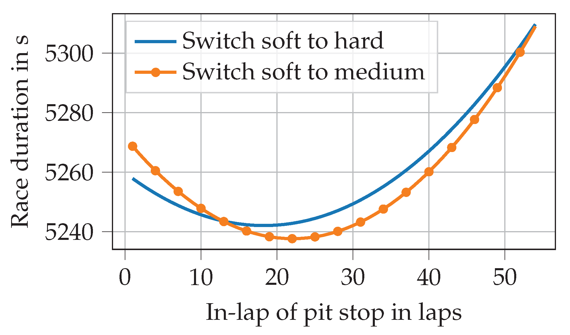
If we imagine a race without opponents or probabilistic influences, we can easily calculate the estimated race duration. Figure 1 illustrates how a variation of the pit stop lap and differences in the choice of tire compounds (either from soft to medium or from soft to hard) influence the race duration of a 1-stop race. In general, a softer compound initially results in faster lap times, but it also degrades faster than a harder compound. Consequently, in this example, if the pit stop took place before lap 13, we would choose to switch to the hard compound.

The simple model of a race without opponents also allows us to explain how full-course yellow (FCY) phases affect strategic decisions. An FCY phase is deployed by race control to reduce the race speed if there is a hazard on the track, e.g., due to an accident. From a strategic perspective, it is essential to know that time lost during a pit stop is significantly less under FCY conditions. This is because it depends on the difference between the time needed to drive from pit entry to pit exit on the track and the time needed to drive through the pit lane. Under FCY conditions, cars drive slower on the track, while going through the pit lane is always speed limited and, therefore, not affected. 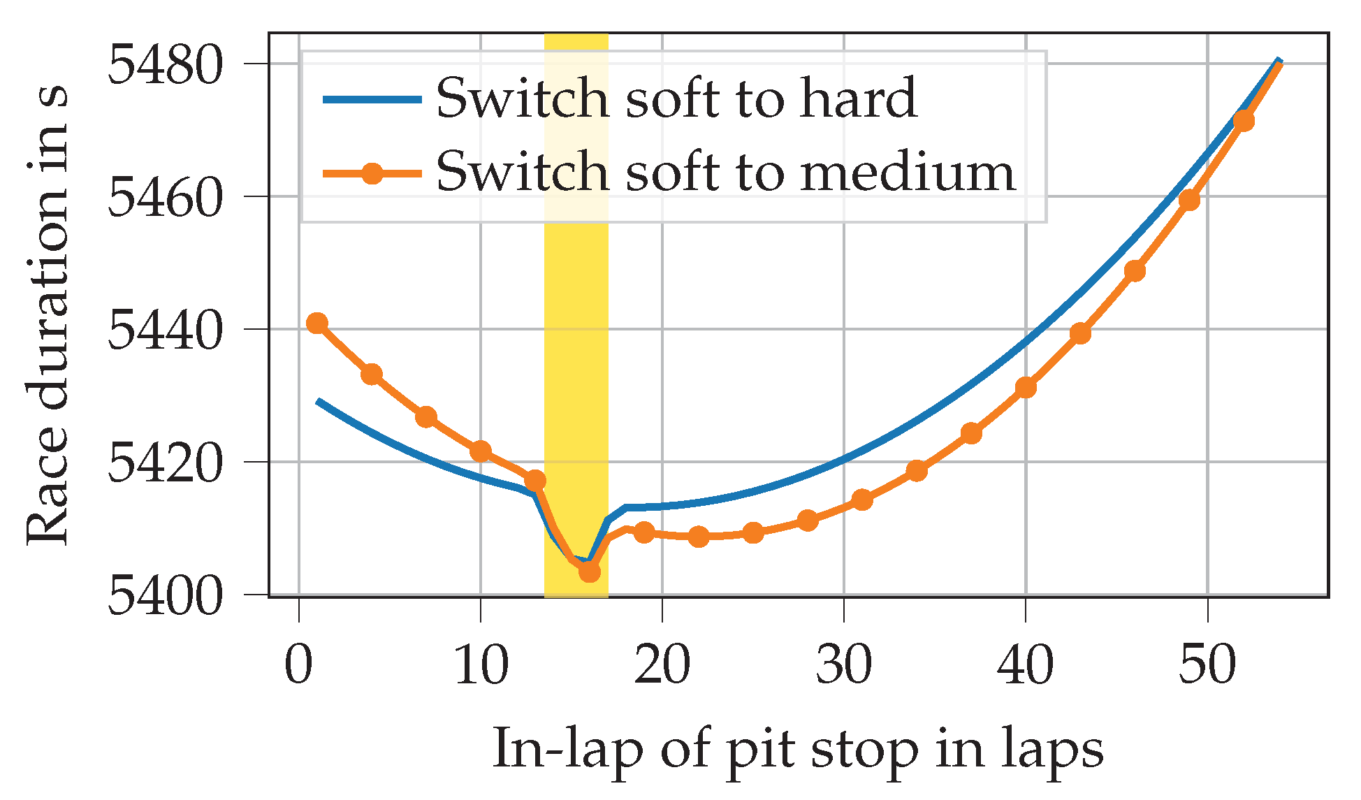Figure 2 illustrates how the optimum pit stop lap changes when an FCY phase commences in the middle of lap 14 and lasts until the end of lap 17.

It is evident that the minimum (i.e., shortest) race duration is achieved by entering the pit in lap 16. This is because the pit stop in-lap and out-lap (the finish line is crossed within the pit lane) are both covered by the FCY phase if the driver enters the pit in lap 16. If the pit stop occurred in lap 17, only the in-lap component would benefit from the reduced time loss during an FCY phase. If, however, the pit stop was made earlier than lap 16, the length of the second stint and thus the tire degradation in that stint would be increased, resulting in a longer race duration. However, we should not forget that the simple model does not include other drivers into consideration, which is why no positions are lost during a pit stop. In reality, most drivers enter the pit directly when the FCY phase commences, for this reason.

In contrast to the simplified model, battles for position are an essential aspect of real-world racing. Race strategy offers several tactical opportunities in this context, such as undercut, overcut, and go long [1], of which the undercut is most prominent. It is used if a driver is stuck behind another driver on the track, i.e., if he is fast enough to follow him, but not fast enough to be able to overtake him directly. By performing an earlier pit stop than the driver in front, the pursuer can attempt to take advantage of having a new set of tires. If he gains enough time before his opponent makes his pit stop, he can pass him indirectly while the opponent is still in the pit lane. The greater the advantage of a new set of tires and the less traffic the pursuer faces after his pit stop, the better this maneuver works. Apart from driver interactions, real-world races are also affected by various probabilistic influences, such as lap time variation and FCY phases. Consequently, comprehensive race simulations (RS) are used to evaluate the outcome of different strategic options.

1.1. Functionality of Race Simulations

In [2], we presented a RS that simulates a race taking into account the most important effects on lap times: tire degradation, burned fuel mass, and interactions between the drivers, i.e., overtaking maneuvers. It simulates the race lap-wise, i.e., lap for lap. In each lap l, it calculates the lap time $t_{\mathrm{lap}}$ for each driver. This is done by adding several time components, see Equation (1) [2]. The base lap time $t_{\mathrm{base}}$ represents the track characteristics. This can be regarded as the minimum lap time that can be achieved by the fastest driver-car combination under optimum conditions. It is increased by $t_{\mathrm{tire}}$ to include the effect of tire degradation (depending on the tire age a and compound c), $t_{\mathrm{fuel}}$ for the effect of fuel mass aboard the car, and $t_{\mathrm{car}}$ and $t_{\mathrm{driver}}$ that represent car and driver abilities. At the start of the race, $t_{\mathrm{grid}}$ adds a time loss that varies in relation to the grid position $p_{\mathrm{g}}$. Pit stops also increase the lap time. This is incorporated by $t_{\mathrm{pit},\mathrm{in}-\mathrm{lap}/\mathrm{out}-\mathrm{lap}}$. The definition of the pit stops, i.e., in-laps, tire compound choices, and the amount of fuel to be added, currently has to be prescribed by the user as an input to the simulation.

$$t_{\mathrm{lap}}\left(l\right)=t_{\mathrm{base}}+t_{\mathrm{tire}}(a,c)+t_{\mathrm{fuel}}\left(l\right)+t_{\mathrm{car}}+t_{\mathrm{driver}}+t_{\mathrm{grid}}(l,p_{\mathrm{g}})+t_{\mathrm{pit},\mathrm{in}-\mathrm{lap}/\mathrm{out}-\mathrm{lap}}\left(l\right)$$

(1)

Consecutive lap times can be summed up to obtain the race time $t_{\mathrm{race}}\left(l\right)$ at the end of a lap as given by

$$t_{\mathrm{race}}\left(l\right)=\sum _{i=1}^l{t}_{\mathrm{lap}}\left(i\right).$$

(2)

A comparison of different drivers’ race times at the end of a lap allows the algorithm to check whether overtaking maneuvers have occurred, which would result in a modification of the lap times of the drivers concerned. When a race is fully simulated, the RS returns each driver’s final race durations as the main output. These inherently include the final positions. In [3], the RS was significantly extended by probabilistic effects, such as lap time variation, variation in pit stop duration, and FCY phases. They are evaluated by performing thousands of simulation runs according to the Monte Carlo principle, resulting in a distribution of the result positions.

There are two applications in which the RS can be used. Before the race, the user is interested in determining a fast basic strategy to start with and assessing several what-if scenarios to prepare him for the race. During the race, the RS can be used to continually re-evaluate the strategy by predicting the race outcomes of different strategic options, starting from the current state.

1.2. Research Goal and Scope

As stated above, the user currently has to insert the pit stop information for all drivers into the RS. This applies to all published race simulations that are known to the authors. This is not only time-consuming, but also requires the user to make a valid estimate of the opponent driver’s race strategies. Besides, user-defined strategies are fixed for the simulated race and can therefore not take advantage of tactical opportunities arising from random events during a race. For example, as described above, it could be beneficial to make a pit stop under FCY conditions. To overcome these limitations, we aim to automate strategy determination by means of software.

Classic optimization methods are hardly applicable in this use case. Firstly, the RS would serve as an objective function for the optimization algorithm. However, the non-linear and discontinuous RS already eliminates many optimization algorithms. Secondly, this variant would again suffer from the problem that the strategy could not be adapted to suit the race situation during the simulated race, as was already the case with the user input. Thirdly, it would not be possible to optimize each driver’s strategy simultaneously, from a selfish perspective. However, this is what happens in reality. Fourthly, the computation time would be high, due to the many RS evaluations required to find the optimum. This is all the more so when one considers that each strategy variant would again require many runs due to the probabilistic effects that are evaluated by Monte Carlo simulation.

The use of stochastic models, e.g., a Markov chain, would be another possibility for the automation of strategy decisions. However, the fact that they are based on transition probabilities has several disadvantages compared to other methods. Firstly, even in situations where a pit stop does not seem reasonable based on the available timing data, stochastic models have a chance to decide in favor of a pit stop because there are few such cases in the training data. An example would be if the tires were replaced due to a defect and not due to wear, e.g., after a collision with another car. Other methods learn the underlying mechanisms, which is why rare cases have much less influence on the decision behavior. Secondly, there is no repeatability in the decisions of stochastic models, which makes no sense if we assume that the race situation reasons the decisions. This also makes it difficult to understand and verify the decision behavior of the model. Thirdly, the available real-world training data is very limited. Therefore, the transition probabilities for rare situations cannot be realistically determined given the enormous number of possible race situations.

It is these aspects that gave us the idea of developing a virtual strategy engineer (VSE) based on machine-learning (ML) methods. These allow us to model relationships between inputs (e.g., tire age) and output (e.g., pit stop decision) that are otherwise hard to determine. The idea is to call the VSE of a driver once per lap to take the relevant strategy decisions (whether or not the driver should make a pit stop, which tires are to be fitted, and whether the car is to be refueled) based on the current race situation, tire age, etc. This concept has several more advantages. Firstly, the VSE could be used for any number of drivers while still behaving selfishly for the corresponding driver. Secondly, most ML methods are computationally cheap during inferencing. Thirdly, the VSE could be used not only in simulation, but also to support time-critical strategy decisions in real-world races without a simulation, e.g., when an FCY phase suddenly occurs.

Our simulation environment and the idea for the VSE can be applied to various types of circuit-racing series. For several reasons, however, our research focuses on the FIA Formula 1 World Championship (F1). This is because it provides vast strategic freedom, since the teams can choose from three different dry tire compounds per race and because it is one of the most popular circuit-racing series. Thus, timing data are publicly available that we can use to create a database (which will be presented in more detail later on) for training ML algorithms. This aspect is crucial, since we have no access to internal team data. Consequently, in this paper, we assume that a pit stop is always performed to fit a new set of tires, since there has not been any refueling in F1 since the 2010 season. For the application in other circuit racing series, the race simulation parameters would have to be adjusted for the respective races. Furthermore, the VSE would have to be re-trained on corresponding real-world timing data. For similar regulations, the presented VSE concept should still be usable. For racing series with clearly different regulations, however, the structure of the VSE would, of course, have to be revised. This would be the case, for example, if refueling was allowed during pit stops.

2. Related Work

This section focuses on the topical background. The ML algorithms are interpreted as tools and are therefore not considered any further. The literature reveals that decision making in sports and sports analytics has become the subject of extensive research during the last two decades. This is due to both the increasing availability of data and the success of ML algorithms that enable meaningful evaluation of data. Possible outcomes of sports analytics include result prediction, performance assessment, talent identification, and strategy evaluation [4]. Consequently, many different stakeholders are interested in such analyses, e.g., bookmakers and betters, fans, commentators, and the teams themselves.

2.1. Analysis Before or After an Event

2.1.1. (American) Football

Predicting the winners and losers of football matches mostly involves the application of ML methods (decision trees, neural networks (NNs), support vector machines) [5,6,7]. Delen et al. [7] found that classification-based predictions work better than regression-based ones in this context. Leung et al. [8] use a statistical approach rather than ML.

2.1.2. Greyhound Racing

Predicting the results of greyhound races was analyzed in several publications [9,10,11]. Various ML methods (decision trees, NNs, support vector machines) outperform human experts in several betting formats.

2.1.3. Horse Racing

Harville [12] uses a purely mathematical approach to determine the probabilities of different outcomes of multi-entry competitions, here horse races. In addition, NNs were applied in predicting the results of horse races [13,14].

2.1.4. Soccer

ML methods also dominate when it comes to result prediction (win, lose, draw) in soccer [15,16,17,18,19]. Joseph et al. [15] found that a Bayesian network constructed by a domain expert outperforms models that are constructed based on data analysis. Tax et al. [17] mention that cross-validation is not appropriate for time-ordered data, which is commonplace in sports. Prasetio et al. [18] combined real-world and video game data to enable improved training of their logistic regression model.

2.1.5. Motorsport

In terms of motorsport, it is mainly the American NASCAR racing series that is investigated in the literature. Graves et al. [20] established a probability model to predict result positions in a NASCAR race. Pfitzner et al. [21] predicted the outcome of NASCAR races using correlation analysis. They found that several variables correlate with result positions, e.g., car speed, qualifying speed, and pole position. Depken et al. [22] found that drivers in NASCAR are more successful in a multi-car team than in a single-car one. Allender [23] states that driver experience and starting position are the most important predictors of NASCAR race results. Stoppels [24] studied predictions of race results in the 2017 F1 season based on data known before the race, e.g., weather and starting grid position. Stergioudis [25] used ML methods to predict result positions in F1.

2.1.6. Various Sports

Result prediction was also investigated for several other sports, generally using NNs or regression analysis. These included swimming [26], basketball [27], hurdle racing [28], javelin throwing [29], and rugby [30].

2.1.7. Broad Result Prediction

In contrast to the previous studies, several publications consider result prediction for more than one sport. McCabe et al. [31] use an NN with input features that capture the quality of sports teams in football, rugby, and soccer. Dubbs [32] uses a regression model to predict the outcomes of baseball, basketball, football, and hockey games. Reviews of available literature and ML techniques for result prediction are available in [4,33]. Haghighat et al. [33] emphasize that there is a lack of publicly available data, making it hard to compare results among different publications.

2.2. In-Event Analysis

2.2.1. Motorsport

The work done by Tulabandhula et al. [34] comes closest to what is pursued in this paper. Using ML methods, they predict the change in position during the next outing (equal to a stint) in NASCAR races on the basis of the number of tires changed in the preceding pit stop. Over 100 possible features were tested, including current position, average position in previous outings, and current tire age. Support vector regression and LASSO performed best, reaching $R^2$ values of 0.4 to 0.5. It was found that “further reduction in RMSE, increase in $R^2$, and increase in sign accuracy may not be possible because of the highly strategic and dynamic nature of racing” ([34], p. 108). The work of Choo [35] is similar to that of Tulabandhula et al. In recent seasons, Amazon [36] applied ML techniques to provide new insights into F1 races for fans. Since they are in a partnership with the F1 organizers, they have access to a vast amount of live data from the cars and the track. Unfortunately, they do not publish how their ML algorithms are set up, trained, and evaluated. Aversa et al. [37] discuss the 2010 F1 season’s final race, in which Ferrari’s decision support system resulted in incorrect conclusions in terms of race strategy. The paper concentrates on the analysis and possible improvements to the decision-making process in the team. Liu et al. [38] combine an NN, which predicts the performance of a Formula E race car, with Monte Carlo tree search to decide on the energy management strategy in Formula E races.

2.2.2. Various Sports

For baseball, Gartheeban et al. use linear regression in [39] and a support vector machine in [40] to decide when a pitcher should be replaced and to determine the next pitch type, respectively. Bailey et al. [41] and Sankaranarayanan et al. [42] apply regression models to predict the match outcome in cricket while the game is in progress. Weber et al. [43] present an approach to model opponent behavior in computer games. They outline that ML algorithms can predict the strategies of human players in a game before they are executed.

2.3. Conclusions

From an engineering perspective, we can conclude that it is mostly two-class (win, lose) and three-class (win, lose, draw) classification problems that are considered in the literature. Many papers emphasize the importance of feature generation, often performed on the basis of domain knowledge. ML algorithms are almost always used, with NNs being increasingly applied in recent years.

From a topical perspective, little literature is available that considers in-event decisions, particularly motorsport. This is surprising, considering the amount of money and data in the sport. The work done by Tulabandhula et al. [34] comes closest to our target. However, it is not applicable in our case, since their algorithm does not predict whether the driver should make a pit stop. The horizon is also limited to a single stint, whereas we have to track the entire race to obtain accurate decisions. Additionally, in NASCAR, only a single tire compound is available. As a consequence, it is necessary to develop a new approach.

3. Methodology

The field of ML covers a vast number of methods. We looked into several classic methods, such as support vector machines and random forests, as well as into NNs. We found that NNs performed much better with our problem than traditional methods, especially in terms of prediction quality, robustness, and comprehensibility. Therefore, we chose to focus on them in this paper. The main emphasis is on NNs trained on real data, a method known as supervised learning. We conclude with a brief outlook towards a reinforcement learning approach based on training in the race simulation.

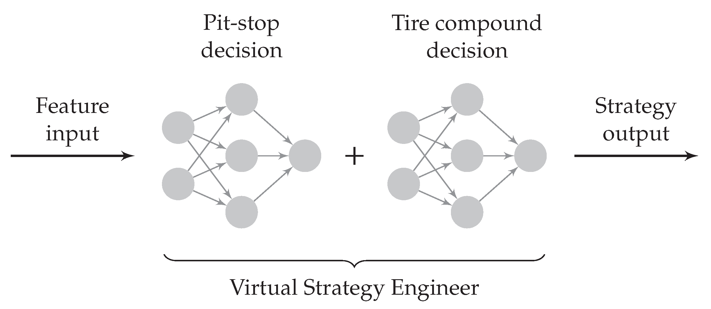
As indicated in Figure 3, we chose to split the strategy decision in the VSE into two parts: the pit stop decision and choice of tire compound. The idea is that one NN first determines whether the driver should make a pit stop. If it decides to make a pit stop, a second NN determines which tire compound should be fitted. The process implies that the choice of the next compound does not influence the pit stop decision. On the downside, this can lead to a slight decrease in the accuracy of the pit stop prediction. On the other hand, the separation facilitates training, allows us to use NN architectures tailored to the specific application, and shortens inference times (as the tire compound choice NN only needs to be invoked if a pit stop is made), which is indeed why we opted for it. Accordingly, after the description of the database, each NN will be given its own separate treatment in the following.

3.1. Formula 1 Database

The training of NNs requires a huge amount of data. The database we created covers the F1 hybrid era from 2014 to 2019. This period is appropriate as the regulations were relatively stable at that time. The data in the database originate from different sources. The basics, such as lap times, positions, and pit stop information, are obtained from the Ergast API [44]. We then added a large amount of information, e.g., the tire compound used in each lap, and FCY phases (start, end, type). It should be noted that the FCY phases in F1 are divided into two types: virtual safety car (VSC) and safety car (SC) phases. During VSC phases, drivers have to reduce their speed, which increases lap times to about 140% of an unaffected time [3]. In SC phases, a real-world car drives onto the race track, which must not be overtaken. This increases the lap times further to about 160% [3].

Table 1. Relevant entries in the laps table of the database. All content refers to the end of the respective lap.

Field	Unit	Description
race_id	–	Unique race ID
lapno	–	Lap number
position	–	Position
driver_id	–	Unique driver ID
laptime	s	Lap time
racetime	s	Race time (cumulated lap times)
gap	s	Distance to race leader
interval	s	Distance to driver in front
compound	–	Current tire compound
tireage	laps	Tire age
pitstopduration	s	Pit stop duration
startlapprog_vsc	–	Lap progress at the beginning of a VSC phase (if VSC starts in current lap)
endlapprog_vsc	–	Lap progress at the end of a VSC phase (if VSC ends in current lap)
age_vsc	laps	Duration of a VSC phase
startlapprog_sc	–	Lap progress at the beginning of an SC phase (if SC starts in current lap)
endlapprog_sc	–	Lap progress at the end of an SC phase (if SC ends in current lap)
age_sc	laps	Duration of an SC phase

gives an overview of the entries in the laps table of the database, which contains the most relevant data. The entire database is available under an open-source license on GitHub (https://github.com/TUMFTM/f1-timing-database).

The database contains 131,527 laps from 121 races. In 4430 of these laps, the drivers entered the pit. The tires were changed in 4087 of these pit stops, which corresponds to 3.1% of all laps. Accordingly, there is a strong imbalance in the data regarding the pit stop decision. This must be taken into consideration when performing training. Besides this, the large number of changes taking place between seasons makes training difficult. For example,

Table 2. Overview of available tire compounds in the seasons 2014 to 2019. The column names are inspired by the 2019 season compound names, so as to enable comparison of the compounds over the years. A1 is the hardest compound, and A7 is the softest.

Season	A1	A2	A3	A4	A5	A6	A7
2014	Hard	Medium	Soft	Supersoft	–	–	–
2015	Hard	Medium	Soft	Supersoft	–	–	–
2016	Hard	Medium	Soft	Supersoft	Ultrasoft	–	–
2017	Hard	Medium	Soft	Supersoft	Ultrasoft	–	–
2018	Superhard	Hard	Medium	Soft	Supersoft	Ultrasoft	Hypersoft
2019	–	C1	C2	C3	–	C4	C5

shows that new softer tire compounds were introduced in 2016 and 2018 [45], while the 2018 superhard and supersoft compounds were no longer used in 2019 [46]. Additionally, tire dimensions were increased for the 2017 season [47]. Another aspect is that the cars are subject to constant development, so their performance cannot be compared, not even between the beginning and end of the same season. Similarly, driver skills evolve as driving experience grows. Furthermore, air and asphalt temperatures differ between races in different years. Lastly, seasons are not always held on the same race tracks or with the same number of races per season. For example, the race in Malaysia was discontinued after 2017. This means that when training the NNs on the entire database, perfect results cannot be expected. However, we cannot train them only with driver, team, race, or season data, since the available amount of data will quickly be insufficient.

It should also be mentioned that the teams cannot choose freely from the tire compounds available in a particular season. For each race, they are given two (2014 and 2015) or three (from 2016) compounds, which are selected by the tire manufacturer depending on the characteristics of the race track from the available compounds stated in Table 2. Consequently, within a particular race, one focuses on the relative differences between the tire compound options soft and medium (2014 and 2015) or soft, medium, and hard (from 2016 onward), regardless of their absolute hardness. To get a feeling for the different durability of the compounds,

Table 3. Comparison of the average tire age (normalized by race length) when tires are changed, depending on the relative compound and season. The values apply to data filtered according to Section 3.2.2.

Seasons	Average Age Hard	Average Age Medium	Average Age Soft
$\le 2015$	–	33.3%	26.8%
$\ge 2016$	38.8%	34.6%	31.6%
Overall	38.8%	34.1%	29.5%

shows the average normalized tire age at the time of a tire change.

3.2. Automation of Pit Stop Decisions Using a Neural Network

There are many factors influencing the decision of what is the right time to make a pit stop. We want the NN to learn the underlying relationships between inputs (features) and output (prediction). Thus, we have to provide it with the relevant features.

3.2.1. Feature Selection

The output feature is selected first, since the choice of input features is easier to follow with a known target.

Output Feature

The output feature determines the type of prediction that we are pursuing: classification or regression. In a classification problem, the NN is trained to decide on one of several possible classes. In our case, this would be pit stop or no pit stop, which is a binary output. In a regression problem, the NN tries to predict a quantity, such as race progress remaining until the next pit stop. Since this feature is not available in the database, we added it manually for a comparison of the two prediction types. In our test, we found that classification works much better than regression. The main reason for this is that our manually added output feature is independent of unexpected race events, since we do not know when the teams would have made their pit stop without the event. Consequently, with a regression output, the NN cannot recognize that a change in the example input feature FCY condition is related to a change in the output feature, as outlined in

Table 4. Comparison of example output features in a classification and a regression approach.

Lap	FCY Condition	Output Feature (Classification)	Output Feature (Regression)
10	Not active	No pit stop	0.1
11	Not active	No pit stop	0.05
12	Active	Pit stop	0.0

. We therefore opted for classification.

Input Features

We tested many different input features that were created on the basis of domain knowledge. These were assessed in an iterative process, since the prediction quality depends on both the feature set and the network architecture.

Table 5. Input feature set for a neural network to take the pit stop decision.

Feature	Type	Value Range	Evaluation Point
Race progress	Numerical	$[0.0,1.0]$	End of previous lap
Tire age progress	Numerical	$[0.0,1.0]$	End of previous lap
Position	Categorical	$\{\mathrm{leader},\mathrm{pursuer}\}$	End of previous lap
Relative compound	Categorical	$\{\mathrm{soft},\mathrm{medium},\mathrm{hard}\}$	Current lap
Race track category	Categorical	$\{1,2,3\}$	– (constant)
FCY status	Categorical	$\{0,1,2,3,4\}$	Current lap
Remaining pit stops	Categorical	$\{0,1,2,3\}$	Current lap
Tire change of pursuer	Categorical	$\{\mathrm{true},\mathrm{false}\}$	End of previous lap
Close ahead	Categorical	$\{\mathrm{true},\mathrm{false}\}$	End of lap before previous lap

contains the input feature set that performs best on our data (the metric will be explained later) in combination with the final NN architecture.

Race progress and tire age progress are numerical features, and the rest are categorical features. Since the races are similar in distance but differ in the number of laps (depending on the track length), both progress features are normalized by the total number of laps of a race. Tire age progress is furthermore processed such that it increases 50% more slowly during VSC and 75% more slowly during SC phases, as the tires are significantly less stressed during FCY phases. The position is split into leader and pursuers. It turned out that the leader often decides differently to his pursuers, e.g., when a safety car appears. Relative compound names are preferred over absolute ones (A1, A2, etc.), as they enable better comparison between different seasons and race tracks. Furthermore, the central compounds A2, A3, A4, and A5 are much more strongly represented in the database, which would cause training issues. The race track category feature was added as an indicator of the absolute level of tire stress on the respective race track. The categorization is given in

Table A1. The race track categorization is based on the hardest absolute tire compound available for the respective race track in the 2019 season. Thus, Category 1 contains tracks with high tire stress, while the stress is lowest in Category 3.

Location	Category
Austin	2
Baku	2
Budapest	2
Catalunya	1
Hockenheim	2
Kuala Lumpur	2
Le Castellet	2
Melbourne	2
Mexico City	2
Monte Carlo	3
Montreal	3
Monza	2
Sakhir	1
Sao Paulo	1
Shanghai	2
Silverstone	1
Singapore	3
Sochi	2
Spa	1
Spielberg	2
Suzuka	1
YasMarina	3

in the Appendix A. It is based on the hardest absolute tire compound available for the respective race track in the 2019 season. Thus, Category 1 contains tracks with high tire stress, whereas the stress is lowest in Category 3. The five possible FCY status values are defined in

Table 6. Explanation of the full-course yellow (FCY) status feature.

FCY Status	Description
0	No FCY phase active
1	First lap of a VSC phase active at the end of the lap
2	Further laps of a VSC phase active at the end of the lap
3	First lap of an SC phase active at the end of the lap
4	Further laps of an SC phase active at the end of the lap

. It is important to distinguish between whether an FCY phase starts in the current lap or has already been active for some time. In most cases, drivers enter the pits in the first lap of an FCY phase. In later laps, there is either a high risk that the phase will end while the driver is still in the pit (VSC phase) or that many positions are lost because the drivers have already queued up behind the safety car (SC phase). The number of remaining pit stops contributes significantly to the prediction quality. With this feature, the NN does not tend to predict any further pit stops after the last stop. We trained the NN for races with one, two, and three pit stops. Based on experience, more than three pit stops only occur in wet conditions or due to technical problems (in the seasons under consideration). In a later section, we will explain how this feature can be determined in a race simulation. The tire change of pursuer feature indicates whether the pursuer of a driver changed his tires in the previous lap, which helps to counteract undercut attempts. This is improved if combined with the close ahead feature, which is true if a driver is a maximum $1.5$ $\mathrm{s}$ ahead of his pursuer.

The features are evaluated at different points. In reality, the decision to make a pit stop during a lap must be taken before the driver passes the pit lane entry. Accordingly, the decision is mostly based on information available at the end of the previous lap. An exception is the close ahead feature. If the pursuer drives into the pit, he loses some time in the in-lap, i.e., before crossing the finish line in the pit lane. Consequently, he will in most cases fall out of the $1.5$ $\mathrm{s}$ window. Since we have no better alternative with the available data, the feature is evaluated based on the lap before the previous lap. There are three features whose values are taken from the current lap: relative compound, remaining pit stops, and FCY status. This is done for the former two to obtain the correct information, even if the tire was changed in the previous lap. The evaluation of the FCY status is always based on the latest information, as also happens in reality, where teams react very quickly to VSC and SC phases.

3.2.2. Pre-Processing

Several filters are applied when fetching the data from the database:

• Wet races are removed, since tire change decisions under such conditions are mainly based on driver feedback and track dampness (which is not included in the data available to us). This is also the reason why wet compounds were not included in the input feature set.
• Data relating to drivers making more than three pit stops in a race are removed, as already explained.
• Data relating to drivers making their final pit stop after a race progress of 90% are removed. Such pit stops are either made in the event of a technical problem or due to the new rule in the 2019 season that states that the driver with the fastest lap time is awarded an extra championship point (if he also finishes within the top 10). Since the car is lightest shortly before the end of a race (due to the burned fuel), there is the best chance for a fast lap time. Accordingly, drivers who are so far ahead towards the end of a race that they would not drop a position by making a pit stop can afford to stop and get a new set of tires. However, we did not want the NN to learn this behavior, since it is specific to the current regulations.
• Data relating to drivers with a lap time above 200 $\mathrm{s}$ or a pit stop duration above 50 $\mathrm{s}$ are removed. Such cases occur in the event of technical problems, damage to the car, or interruption of the race.
• Data relating to drivers with a result position greater than ten are removed. This is done in order to train the NN on successful strategies only. Of course, a finishing position within the top ten is no guarantee of a good strategy. However, as top teams have more resources, we assume that they tend to make better decisions. This does not introduce bias into the training data, since there are no features in the set that would subsequently be underrepresented, as would be the case with team names, for example.

Applying all the filters results in 62,276 entries (i.e., laps) remaining. The earliest race data presented to the NN are from the end of the first lap. This is because some features, such as the ahead value, are not available before the start of the race. Consequently, the first pit stop decision can be taken for lap two. However, as pit stops in the first lap are not generally made on the basis of worn tires but due to technical problems, this does not cause any issues.

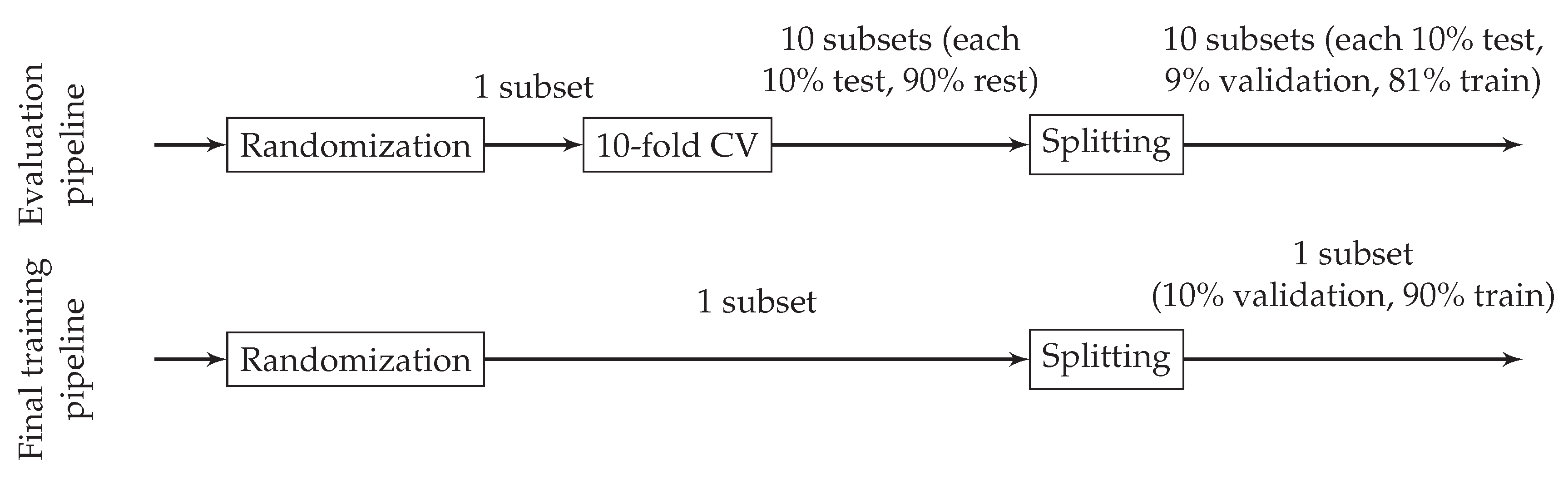
Further on in the process, specified test races are separated from the data to exclude them from the training. Then, the pre-processor removes the mean and normalizes the range of numerical features. Categorical features are one-hot encoded. Next, the data are split into subsets for training, validation, and testing (in the evaluation pipeline) or training and validation (in the final training pipeline), as shown in Figure 4. The training section refers to the training of the NN. The validation section is used to recognize overfitting during training, which ends the training process (‘early stopping’). The test part is used to evaluate the prediction quality of the trained NN. Final training takes place without a test part to maximize the amount of training data available. When evaluating different NN architectures and feature sets, we apply 10-fold cross-validation to obtain a reliable statement regarding prediction quality. During cross-validation and splitting, subsets are created in such a way that they preserve the percentage of samples for each class (‘stratification’), which is essential with imbalanced data.

3.2.3. Metrics

The most common metric used to assess ML algorithms is accuracy. However, it is not appropriate in the case of a binary classification problem with imbalanced data because it places too little focus on the positive class (in our case, pit stop). Precision and recall are better choices. Precision represents the fraction of correct positive predictions. Recall represents the fraction of the positive class that was correctly predicted. For example, if the NN predicts a total of four pit stops, of which three are correct, then the precision is $0.75$. If there are ten pit stops in the training data, then the recall is $0.3$. Usually, there is a trade-off between precision and recall: an increase in one results in a decrease in the other. Since both measures are of similar relevance to us, we decided to take the $F_1$ score introduced in Equation (3) [48]. This is the harmonic mean of precision p and recall r and, therefore, does not reach a high value if one of the two is low.

$$F_1=2\frac{p·r}{p+r}$$

(3)

3.3. Automation of Tire Compound Decisions Using a Neural Network

As with the pit stop decision, we need to choose features that allow the NN to learn the relevant relationships for the decision on which tire compound should be selected during a pit stop.

3.3.1. Feature Selection

As before, the output feature is explained first.

Output Feature

The NN shell predicts the relative compound that is chosen during a pit stop, i.e., soft, medium, or hard. Due to the limited amount of training data, we decided to consider the 2014 and 2015 seasons, in which only two compounds were available per race, by using a special input feature, instead of training a separate NN. In contrast to the pit stop decision, this is a multi-class classification problem. Consequently, there are three neurons in the NN’s output layer, of which the compound with the highest probability is chosen.

Input Features

The feature set for the tire compound decision is much smaller than for the pit stop decision, as can be seen from

Table 7. Input feature set for a neural network to take the compound decision.

Feature	Type	Value Range	Evaluation Point
Race progress	Numerical	$[0.0,1.0]$	End of previous lap
Remaining pit stops	Categorical	$\{0,1,2,3\}$	Current lap
Relative compound	Categorical	$\{\mathrm{soft},\mathrm{medium},\mathrm{hard}\}$	Current lap
Race track	Categorical	$\{\mathrm{Austin},\mathrm{Baku},\dots ,\mathrm{Yas}\mathrm{Marina}\}$	– (constant)
Fulfilled second compound	Categorical	$\{\mathrm{true},\mathrm{false}\}$	Current lap
Number of avail. compounds	Categorical	$\{2,3\}$	– (constant)

. The features race progress, remaining pit stops, and relative compound are already familiar from the pit stop decision. For the compound decision, the race track feature is preferable to the race track category due to the improved prediction quality. This does not lead to overfitting in this case, as training is still carried out across the different seasons and teams. For better generalizability, however, the race track category could also be used (at the expense of a worse prediction quality). The fulfilled second compound feature indicates whether a driver has already used two different compounds in a race. The regulations in F1 require this. The last feature, number of available compounds, is two for the seasons prior to 2016 or three from 2016 onwards. In the former case, the NN learns to neutralize the hard output neuron very well.

3.3.2. Pre-Processing

Here, data filtering is less strict than with the pit stop decision. Since the available amount of training data is much smaller, we cannot remove too much of it. Only the 4087 laps with a tire change are relevant. As with the pit stop decision, the entries are filtered for races in dry conditions with one to three pit stops. Furthermore, data relating to a result position above 15 are removed. This results in 2757 entries remaining.

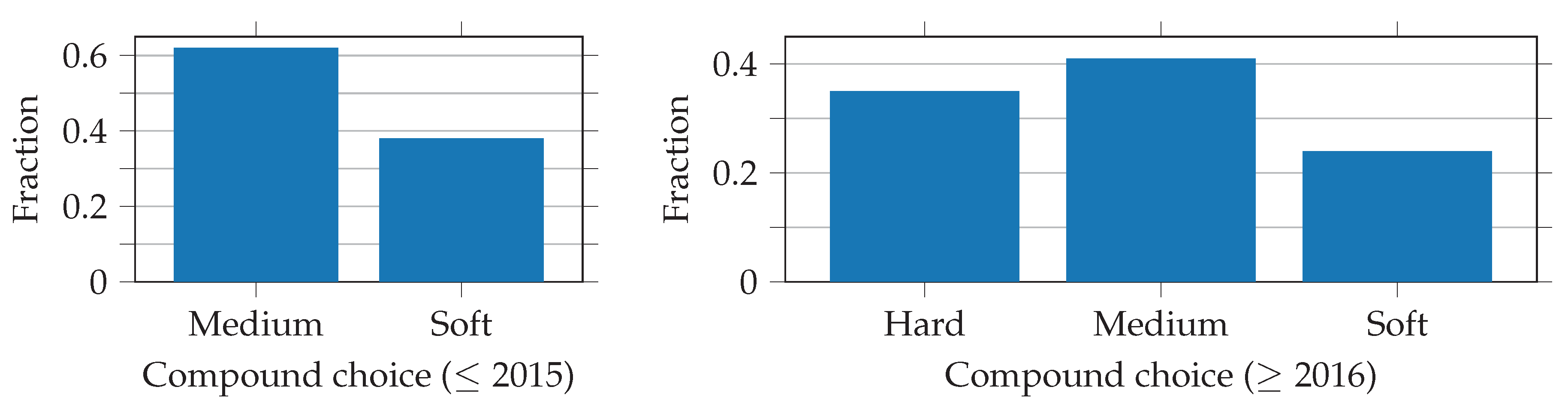
Pre-processing, including splitting the data into subsets, is similar to that of the pit stop decision. The data are, however, not as imbalanced. Figure 5 shows an overweight on the medium compound decisions. This is because the regulations force the top ten drivers to start the race on the tires on which they set the fastest lap time in the second part of the qualifying. In most cases, this means that they have to start on the soft compound, which is why they do not often change back to the soft compound during the race. The imbalance in the data is small enough that no further action is needed.

3.3.3. Metrics

The goal is to make as many correct compound choice predictions as possible. Accordingly, accuracy is the metric used in evaluating the NN. It represents the fraction of correct predictions.

3.4. Optimization of Basic Race Strategies

We mentioned above that the remaining pit stops feature significantly improves the prediction quality of the VSE, which is why it was included in the input feature sets. Consequently, if the VSE is integrated into the race simulation, the intended number of pit stops for a race must be determined. As mentioned in the introduction, if we consider the interactions between drivers and probabilistic influences, there is no optimum strategy. However, if these effects are omitted and if we assume some simplifications (which will be explained in the following), it can be done using a two-step approach:

• Determination of all possible tire compound combinations for each reasonable number of pit stops
• Determination of the optimum stint lengths for each of those combinations

Once the minimum race duration is known for each compound combination, we can compare them and take the fastest.

3.4.1. Determination of all Possible Tire Compound Combinations

As mentioned above, the optimum number of pit stops in a dry F1 race without any unforeseen events is between one and three (in the seasons considered). Together with the three relative compounds per race, soft (S), medium (M), and hard (H), we can now determine all the possible combinations. The regulations require every driver to use two different compounds per race. This reduces the number of possible combinations. Furthermore, in a race without opponents, the order of the tire compounds, for example, if the driver first uses the hard compound and then the soft one or vice versa, is irrelevant. This is valid if we assume that tire degradation is independent of changing track conditions and the change in vehicle mass (due to burned fuel). The former statement can be explained by the fact that the track has already been driven in three training sessions and the qualifying. The latter statement is based on the fact that the fuel mass is at most about 13% of the vehicle mass (in the 2019 season). We therefore assume that it does not influence the result too much. This is supported by the assumption that, with reduced mass, the drivers simply drive at higher accelerations, thus keeping tire degradation at a similar level. We thus obtain the following possible combinations (referred to from this point as ‘sets’):

• 1-stop strategies: SM, SH, MH
• 2-stop strategies: SSM, SSH, SMM, SMH, SHH, MMH, MHH
• 3-stop strategies: SSSM, SSSH, SSMM, SSMH, SSHH, SMMM, SMMH, SMHH, SHHH, MMMH, MMHH, MHHH

As mentioned, the start compound is fixed for each driver who qualifies in the top ten. In this case, the number of sets decreases even further. In general, however, 22 possible sets remain per driver.

3.4.2. Determination of Optimum Stint Lengths for Each Set

Optimum stint lengths are those with the minimum race duration for the respective set. When omitting driver interactions, a driver’s race duration is simply the sum of his lap times. Looking at Equation (1), we find that there are four lap-dependent elements: $t_{\mathrm{grid}}$, $t_{\mathrm{fuel}}$, $t_{\mathrm{pit},\mathrm{in}-\mathrm{lap}/\mathrm{out}-\mathrm{lap}}$, and $t_{\mathrm{tire}}$. The grid time loss and time loss due to fuel mass occur independently of the race strategy and can therefore be omitted when determining optimum stint lengths. For a known amount of pit stops per set, pit time losses are also fixed. Thus, under the afore mentioned assumptions, the race duration of a given set depends only on the time loss due to tire degradation and, therefore, on the stint lengths.

A set’s optimum stint lengths can either be determined by calculating the race durations for all possible combinations of stint lengths ( 1 lap/ 69 laps, 2 laps/ 68 laps, etc. in a race with 70 laps), or, in the case of a linear tire degradation model, by solving a mixed-integer quadratic optimization problem (MIQP). Solving the MIQP is much faster, notably with the 2- and 3-stop strategies. Especially with no very detailed timing data, the linear degradation model is mostly used anyway, as it is the most robust model. The formulation of the MIQP is introduced in the following.

With $l_{\mathrm{tot}}$ being the total number of laps in a race, the objective of the MIQP reads as follows:

$$min{t}_{\mathrm{race}}\left(l_{\mathrm{tot}}\right)\widehat{=}min\sum _{l=1}^{l_{\mathrm{tot}}}{t}_{\mathrm{tire}}\left(l\right).$$

(4)

Splitting the race into a fixed number of stints N ($\mathrm{pit}\mathrm{stops}=N-1$) with stint index i, compounds $c_i$ and stint lengths ${\alpha }_i$ as optimization variables, the problem can be formulated as follows:

$$\begin{array}{cccc}\hfill & \underset{\begin{array}{c}\hfill {\alpha }_1\cdots {\alpha }_N\end{array}}{min}\hfill & \hfill & \sum _{i=1}^N\sum _{a=1}^{{\alpha }_i}{t}_{\mathrm{tire}}(a,c_i)\hfill \\ \hfill & \mathrm{subject}\mathrm{to}\hfill & \hfill & \sum _{i=1}^N{\alpha }_i=l_{\mathrm{tot}}\hfill \\ \hfill & \hfill & \hfill & {\alpha }_i\in {\mathbb{N}}^{+}\forall 1\le i\le N.\hfill \end{array}$$

(5)

Next, we introduce the linear tire degradation model. Thus, the time loss $t_{\mathrm{tire}}$ is determined by tire age a and two coefficients $k_0$ and $k_1$, which are dependent on the tire compound c:

$$t_{\mathrm{tire}}(a,c)=k_0\left(c\right)+k_1\left(c\right)·a.$$

(6)

In general, a softer tire is faster in the beginning ($k_0$ is smaller than for a harder compound), but also displays a faster degradation ($k_1$ is higher than for a harder compound). Inserting the tire degradation model into Equation (5), we obtain:

$$\sum _{i=1}^N\sum _{a=1}^{{\alpha }_i}{t}_{\mathrm{tire}}(a,c_i)=\sum _{i=1}^N\left(k_0\left(c_i\right)·{\alpha }_i+k_1\left(c_i\right)\sum _{a=1}^{{\alpha }_i}a\right).$$

(7)

Using the Gaussian sum for the last part and rewriting $k_0\left(c_i\right)$ and $k_1\left(c_i\right)$ as $k_{0,i}$ and $k_{1,i}$, respectively, gives:

$$\sum _{i=1}^N\sum _{a=1}^{{\alpha }_i}{t}_{\mathrm{tire}}(a,c_i)=\sum _{i=1}^N\left(k_{0,i}·{\alpha }_i+k_{1,i}\left(\frac{1}{2}{\alpha }_i^2+\frac{1}{2}{\alpha }_i\right)\right).$$

(8)

For the case that the tires are not new at the start of a stint, for instance for the top ten starters, a starting age $a_{\mathrm{s},i}$ is introduced into the formulation. Accordingly, ${\alpha }_i$ is replaced by ${\alpha }_i+a_{\mathrm{s},i}$ and the offset loss of $a_{\mathrm{s},i}$ is subtracted:

$$\begin{array}{cc}\hfill \sum _{i=1}^N\sum _{a=1}^{{\alpha }_i}{t}_{\mathrm{tire}}(a,c_i,a_{\mathrm{s},i})=\sum _{i=1}^N& \left(k_{0,i}\left({\alpha }_i+a_{\mathrm{s},i}\right)+k_{1,i}\left(\frac{1}{2}{\left({\alpha }_i+a_{\mathrm{s},i}\right)}^2+\frac{1}{2}\left({\alpha }_i+a_{\mathrm{s},i}\right)\right)\right.\hfill \\ \hfill & \left.-\left(k_{0,i}·a_{\mathrm{s},i}+k_{1,i}\left(\frac{1}{2}{a}_{\mathrm{s},i}^2+\frac{1}{2}{a}_{\mathrm{s},i}\right)\right)\right).\hfill \end{array}$$

(9)

Switching to vector notation, we obtain the final formulation:

$$\begin{array}{cccc}\hfill & \underset{\begin{array}{c}\hfill {\alpha }_1\cdots {\alpha }_N\end{array}}{min}\hfill & \hfill & {\overrightarrow{\alpha }}^{T}H\overrightarrow{\alpha }+f^T\overrightarrow{\alpha }\hfill \\ \hfill & \mathrm{subject}\mathrm{to}\hfill & \hfill & \sum _{i=1}^N{\alpha }_i=l_{\mathrm{tot}}\hfill \\ \hfill & \hfill & \hfill & {\alpha }_i\in {\mathbb{N}}^{+}\forall 1\le i\le N,\hfill \end{array}$$

(10)

where

$$\begin{array}{cc}\hfill H& =\left[\begin{array}{cccc}0.5·k_{1,1}& 0& \cdots & 0\\ 0& 0.5·k_{1,2}& \cdots & 0\\ ⋮& ⋮& \ddots & ⋮\\ 0& 0& \cdots & 0.5·k_{1,N}\end{array}\right],\hfill \end{array}$$

(11)

$$\begin{array}{cc}\hfill f& =\left[\begin{array}{c}{k}_{1,1}(0.5+a_{\mathrm{s},1})+k_{0,1}\\ ⋮\\ k_{1,N}(0.5+a_{\mathrm{s},N})+k_{0,N}\end{array}\right].\hfill \end{array}$$

(12)

Since the total number of laps in a race is known, the length of the last stint can be calculated by subtracting the sum of the lengths of the previous stints from it. This alternative formulation reduces the number of optimization variables by one. However, it causes coupling terms in H, making it more difficult to automatically create the matrix in relation to a given number of pit stops. We therefore opted for the decoupled version.

4. Results

First, the optimization of a basic race strategy is presented. Then, the results of the neural networks are discussed.

4.1. Optimization of Basic Race Strategies

We used ECOS_BB, which is part of the CVXPY Python package [49], to solve the MIQP. The computation time for the 22 sets in an exemplary 55 laps race is about 150 $\mathrm{m}$$\mathrm{s}$ on a standard computer (Intel i7-6820HQ). This includes the time needed for creating the sets, setting up the optimization problem, and performing the post-processing. In comparison, the computation time needed for a brute-force approach is about 20 $\mathrm{s}$. However, should we wish to use a different tire degradation model or take into account further lap-dependent effects, it is also a valid option.

The results of the exemplary 1-stop race shown in Figure 1 were calculated using the brute-force method by simulating all possible combinations of stint lengths. Solving the MIQP for the parameters in

Table 8. Parameters of an example race used to optimize the basic race strategy.

Option	Value
Number of laps in the race	$l_{\mathrm{tot}}=55laps$
Minimum number of pit stops	1
Maximum number of pit stops	3
Start compound	Soft
Tire age at race start	$a_{\mathrm{s}}=2laps$
Degradation model parameters (hard)	$k_0=1.2\mathrm{s}$, $k_1=0.016\mathrm{s}/lap$
Degradation model parameters (medium)	$k_0=0.5\mathrm{s}$, $k_1=0.05\mathrm{s}/lap$
Degradation model parameters (soft)	$k_0=0.0\mathrm{s}$, $k_1=0.09\mathrm{s}/lap$

results in the following optimum stint lengths for the two compound combinations in the figure:

• S for 22 laps + M for 33 laps resulting in a race duration of $5237.65$ $\mathrm{s}$
• S for 18 laps + H for 37 laps resulting in a race duration of $5242.07$ $\mathrm{s}$

Checking the results against Figure 1 proves that these are the fastest stint length combinations. The fastest 2-stop and 3-stop strategies for this race lead to race durations of $5240.95$ $\mathrm{s}$ and $5252.23$ $\mathrm{s}$, respectively. Consequently, the 1-stop strategy is, in this case, also the fastest overall.

The intention behind determining the fastest basic strategy is that it can be used as a basis for the remaining pit stops feature. We therefore stipulated that each additional pit stop must provide an advantage of at least 2 $\mathrm{s}$ for us to consider the respective strategy to be the fastest basic strategy. This is because, in reality, with every pit stop there is the risk of losing significantly more time than planned, for instance if the tires cannot be fastened immediately. Consequently, an additional pit stop must provide a considerable advantage to outweigh the extra risk.

4.2. Automation of Pit Stop Decisions Using a Neural Network

4.2.1. Choice of Neural Network Hyperparameters

We use TensorFlow [50] and the Keras API to program the NNs in Python. Training is performed until there is no decrease in loss on the validation data for five consecutive iterations (‘early stopping with patience’). For selecting the hyperparameters, we started with recommendations from Geron [48], evaluated many different combinations, and compared them in terms of their prediction quality, i.e., $F_1$ score. The parameters finally chosen are given in

Table 9. Hyperparameters of the neural network for the pit stop decision.

Hyperparameter	Value
Number of hidden layers	3
Number of neurons per layer	64
Activation functions	ReLU (hidden layers), sigmoid (output layer)
L2 regularization	0.0005
Optimizer	Nadam
Loss function	Binary cross entropy
Training class weights	no pit stop: 1, pit stop: 5
Training batch size	256

.

The resulting feed-forward NN (FFNN) consists of three fully connected hidden layers of 64 neurons each. In addition to early stopping, L2 regularization is applied to decrease the tendency of overfitting. Class weights are used to increase the loss due to incorrect predictions of the pit stop class, which forces the NN to improve on these predictions during training. Otherwise, it would mostly predict no pit stop, simply because this already results in a minimum loss due to the imbalanced data. The batch size is chosen so large to have a decent chance that each batch contains some pit stops. With these hyperparameters, an average of $F_1\approx 0.35$ is reached on the test data in the evaluation pipeline.

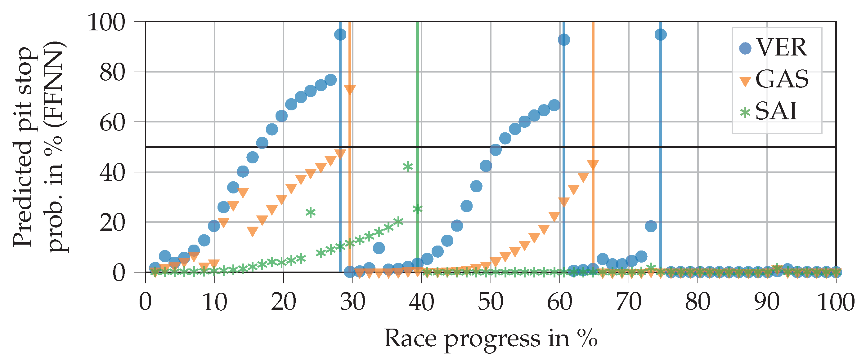
Figure 6 shows the progressions of the NN output for three drivers when inserting real data from the 2019 Brazilian Grand Prix that was excluded from the training data. The output can be interpreted as the predicted pit stop probability. One can generally observe slightly s-shaped curves that drop back down towards zero once the real pit stops have taken place. Several jumps are visible, which are caused by changes in position, FCY status, tire changes of pursuers, and the close ahead feature. The massive jump at Verstappen’s last pit stop (at a race progress of about 75%), for example, is caused by a safety car phase. It can also be seen that the NN output remains consistently around zero after the last pit stop of a race.

The plot helps to explain why the FFNN does not achieve a better $F_1$ score. For example, the NN already predicts Verstappen’s first and second pit stops for eight laps and six laps respectively, before they have taken place. In contrast, two stops by Sainz and Gasly are not predicted (in fact, they would be predicted a few laps too late). Similar problems occur with other races. We conclude that, in principle, the FFNN captures the relationships between inputs and outputs well. However, it does not succeed in sufficiently delaying the increase in output probability during an ordinary race progress, while still allowing it to increase quickly in the case of sudden events, e.g., FCY phases. This would require input data from more than a single lap.

We therefore switched to recurrent neural networks (RNNs), which operate with time-series input data. Their neurons store an internal state, which allows them to learn relationships between consecutive steps. In our case, we insert series of consecutive laps. Pre-processing of these series is as described in Section 3.2.2. Instead of a single lap, units of several consecutive laps are processed with the same pipeline. The only difference is that time series that include laps before the first lap must be artificially filled with ‘neutral values’, cp.

Table 10. Example time series input data for a length of 4 laps showing how values before lap 1 are artificially filled with ‘neutral values’.

Feature	Lap -1	Lap 0	Lap 1	Lap 2
Race progress	0.0	0.0	0.02	0.04
Tire age progress	0.04	0.04	0.06	0.08
Position	3	3	2	2
Relative compound	Soft	Soft	Soft	Soft
Race track category	2	2	2	2
FCY status	0	0	0	0
Remaining pit stops	2	2	2	2
Tire change of pursuer	False	False	False	False
Close ahead	False	False	True	True

.

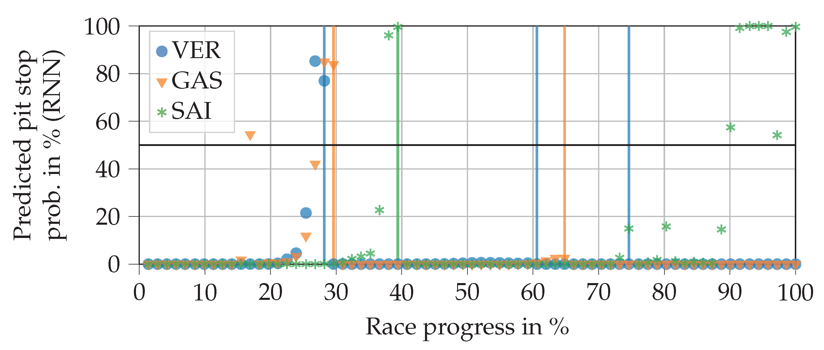
As with the FFNN, many different architectures were tested. We found that pure RNNs can reach high scores on the test data ($F_1\approx 0.9$), but tend to output many incomprehensible predictions. An example of this is given in Figure 7. In particular, Sainz’ predictions in the last part of the race are clearly wrong, since the remaining pit stops feature is zero there. This demonstrates that the $F_1$ score alone has little significance. The predictions of the RNN jump strongly from lap to lap, which is why it predicts significantly less false positives and false negatives than the FFNN, where the predicted probability increases slowly but steadily. However, as the example shows, the pit stop predictions of the RNN are often placed completely incorrectly. This is much worse for making automated pit stop decisions than predicting the pit stop just a few laps too early or too late, as was the case with the FFNN.

We therefore combined the advantages of both types by creating a hybrid NN. The following procedure gave the best results in our tests. The FFNN is first created and trained as described. Then a new model with an equivalent structure to that of the FFNN is created, and a single LSTM (long short-term memory) neuron is added after the original output. Subsequently, the weights for all layers that existed in the FFNN are copied to the hybrid NN and marked as untrainable. Finally, the hybrid NN is trained with data sequences. Only the weights of the LSTM neuron are then adjusted. It thus learns to modify the output of the FFNN such that its predictions become increasingly accurate.

Table 11. Hyperparameters of the neural network for the pit stop decision (RNN section).

Hyperparameter	Value
Number of RNN neurons	1
RNN neuron type	LSTM
Sequence length	4 laps

gives an overview of the additional hyperparameter choices. More than one RNN neuron as well as other neuron types did not result in an improvement in prediction quality. We found that a sequence length of four laps provides the best compromise between prediction quality and inference time. Increasing this to five laps would, for example, increase the inference time by about 10% for a barely measurable improvement in prediction quality. The final configuration achieved an average score of $F_1\approx 0.59$ on the test data in the evaluation pipeline.

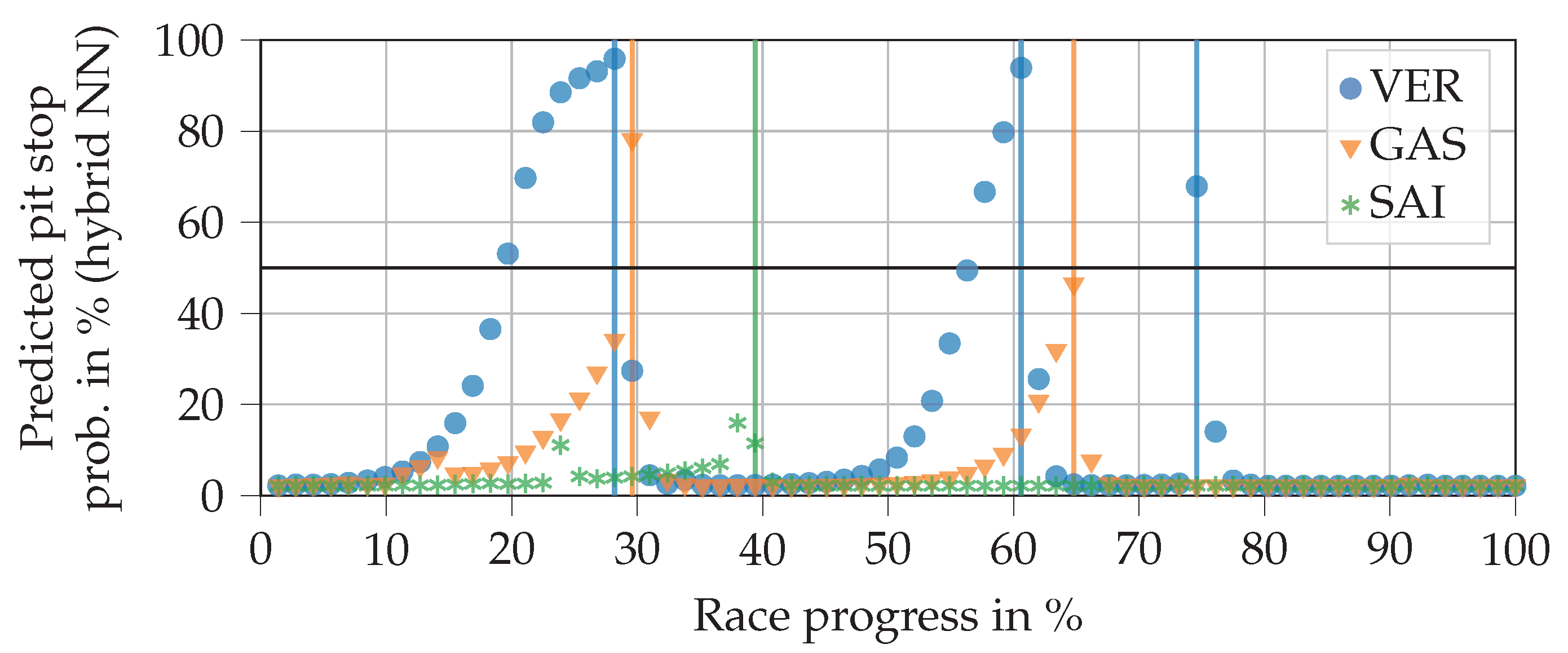
Figure 8 reveals a resulting plot shape of the hybrid NN output resembling a hockey stick. Compared to the FFNN, for example, the curves rise later and more steeply for Verstappen. Accordingly, there is a smaller number of false positives. As can be seen from Verstappen’s last pit stop, which was triggered by a safety car phase, the hybrid NN can pass through sudden jumps of the FFNN section despite the LSTM cell. Compared to pure RNN, the predictions of the hybrid NN can be understood far better. In this example, the hybrid NN does not improve on the two pit stops by Sainz and Gasly compared to the FFNN. However, at least for Gasly’s second stop, the predicted probability would have exceeded 50% only one lap later. The plot also shows that the output does not drop back down to zero directly after a pit stop, unlike with the FFNN. This is due to the LSTM cell. However, we have not observed any case in which the value remains above the 50% line (even in ‘worst case scenarios’).

Table 12. Confusion matrix of the predictions of the final trained pit stop decision NN on the entire database (filtered according to Section 3.2.2).

		Prediction
		No pit stop	Pit stop
Truth	No pit stop	57,836	2048
	Pit stop	537	1855

contains the confusion matrix when the final trained hybrid NN predicts the pit stops on the entire database (filtered according to Section 3.2.2). It can be seen that there are 2048 false positives that are mostly caused by the fact that pit stops are often already predicted for several laps before they actually take place. Overall, 537 pit stops happen without the NN predicting them. This is caused by cases that are either atypical (e.g., unusual early pit stops) or cannot be fully explained by the existing features. Despite the worse $F_1$ score, we consider the hybrid NN superior to the RNN due to its more comprehensible decision behavior.

4.2.2. Analysis of Feature Impact

To examine the plausibility of the final trained NN, we checked the predictions for real-world races. We also investigated its reactions to variations in single input features and determined whether they matched expectations. An example 1-stop race with standard values according to

Table 13. Standard values used to create the example race for the feature impact analysis of the pit stop decision NN.

Feature	Standard Value
Race progress	$[0.0,1.0]$
Tire age progress	$[0.0,1.0]$
Position	2 (pursuer)
Relative compound	Soft
Race track category	2
FCY status	0
Remaining pit stops	1
Tire change of pursuer	False
Close ahead	False

was created for this purpose. Three example analyses are presented in the following.

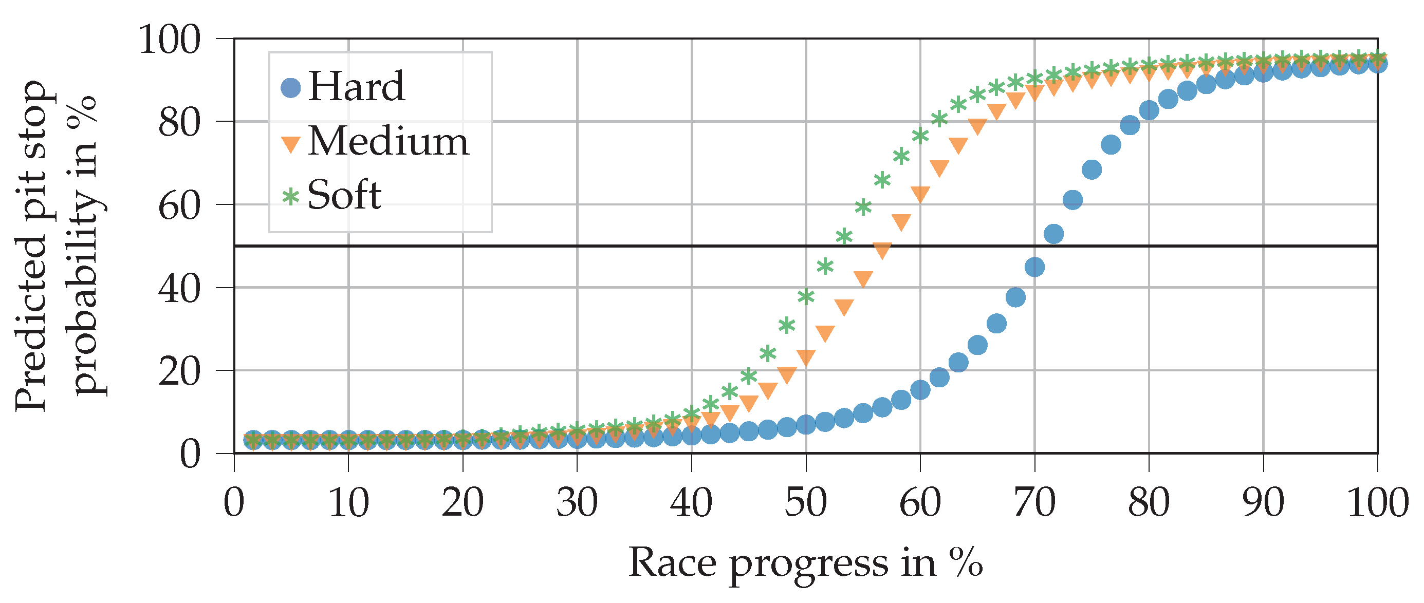
Figure 9 shows the predictions for all three relative compounds when the driver does not make a pit stop. As expected, pit stop probabilities increase steadily until the end of the race. It is also in line with expectations that the soft compound reaches the 50% line first, followed by medium and then hard. It seems surprising that the pit stops are not generally predicted earlier, so that the values match those in Table 3. This can be explained by the fact that many pit stops, in reality, are triggered not only by tire age but also by other factors, e.g., FCY phases. There are no such triggers in our exemplary race.

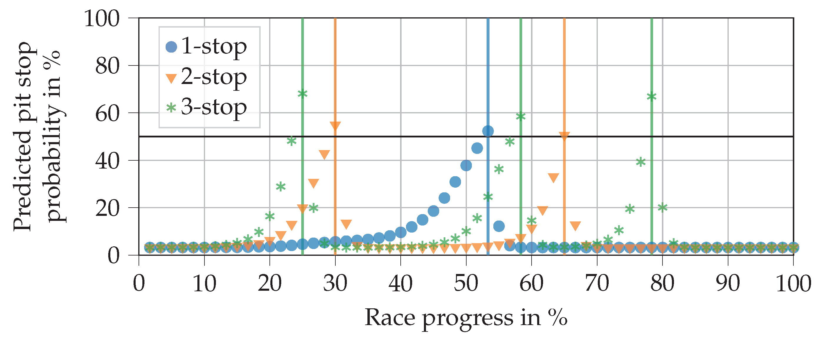
Figure 10 contains the prediction curves for a 1-, 2-, and 3-stop race respectively (varying the remaining pit stops feature). In this example, the pit stops are performed as soon as the predicted probability exceeds 50%. The soft compound is replaced by the medium compound in the first pit stop to comply with regulations. In subsequent pit stops, the soft compound is fitted. The pit stop in the 1-stop race takes place rather late on, considering that the soft compound is used in the first stint. This was already reasoned for the previous plot. In the 2-stop race, the first stop is placed at a race progress of 30%, which meets our expectations. With a length of 35% race progress each, the second and third stints are equivalently long. Knowing that the middle stint is run on medium and the last on soft, we would expect the middle stint to be longer. However, the NN does not know which compound will be fitted next, which is a disadvantage of the separated decision process. The 3-stop race decisions fit in well with expectations. The second stint on medium tires is the longest, while all others are relatively short.

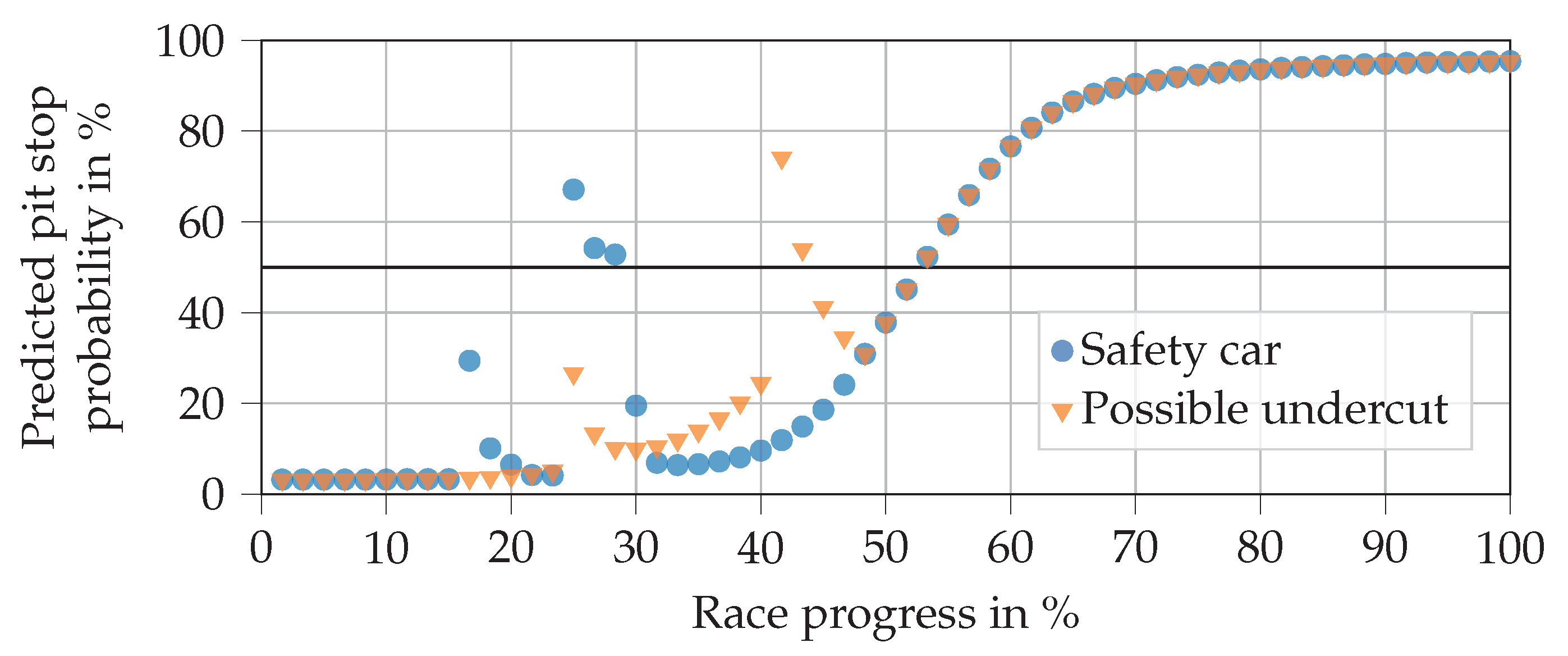
Figure 11 shows the predictions when an SC is deployed in laps 10 and 15, each with a duration of three laps. A possible undercut situation can also be seen in laps 15 and 25. This is done by setting the tire change of pursuer feature to true in these laps along with the close ahead feature being set to true until lap 25. It can be seen that the early SC phase at a race progress around 17% does not trigger a pit stop, whereas the second one does. This is in line with expectations since, in reality, drivers often refrain from entering the pits if an SC phase is deployed at the beginning of a race, when the tires are still fresh. From the predictions with undercut attempts, we can see that the NN reacts well and decides for a pit stop if the attempt is close to a pit stop that is planned anyway.

4.3. Automation of Tire Compound Decisions Using a Neural Network

4.3.1. Choice of Neural Network Hyperparameters

As with the pit stop decision, many hyperparameter sets were trained and compared.

Table 14. Hyperparameters of the neural network for the tire compound decision.

Hyperparameter	Value
Number of hidden layers	1
Number of neurons per layer	32
Activation functions	ReLU (hidden layer), softmax (output layer)
L2 regularization	0.001
Optimizer	Nadam
Loss function	Sparse categorical cross entropy
Training batch size	32

gives an overview of the chosen values. The NN is established with a single layer of 32 neurons. The loss and activation functions of the output layer are adapted to the case of three possible compound choices. In the final configuration, we achieved an average accuracy of $acc\approx 0.77$ on the test data in the evaluation pipeline.

Table 15. Confusion matrix of the predictions of the final trained compound choice NN on the entire database (filtered according to Section 3.3.2).

		Prediction
		Hard	Medium	Soft
Truth	Hard	444	95	62
	Medium	75	1123	147
	Soft	39	130	642

shows the confusion matrix for the predictions of the final trained NN on the entire database (filtered according to Section 3.3.2). As the accuracy already indicates, the majority of decisions are correctly predicted.

Figure 12 visualizes the NN output using the real input data for Gasly in the 2019 Brazilian Grand Prix. As can be seen, Gasly started with the soft compound, then changed to a set of medium tires, switching back to soft tires for the final stint. In this example, the NN predicts both compound choices correctly.

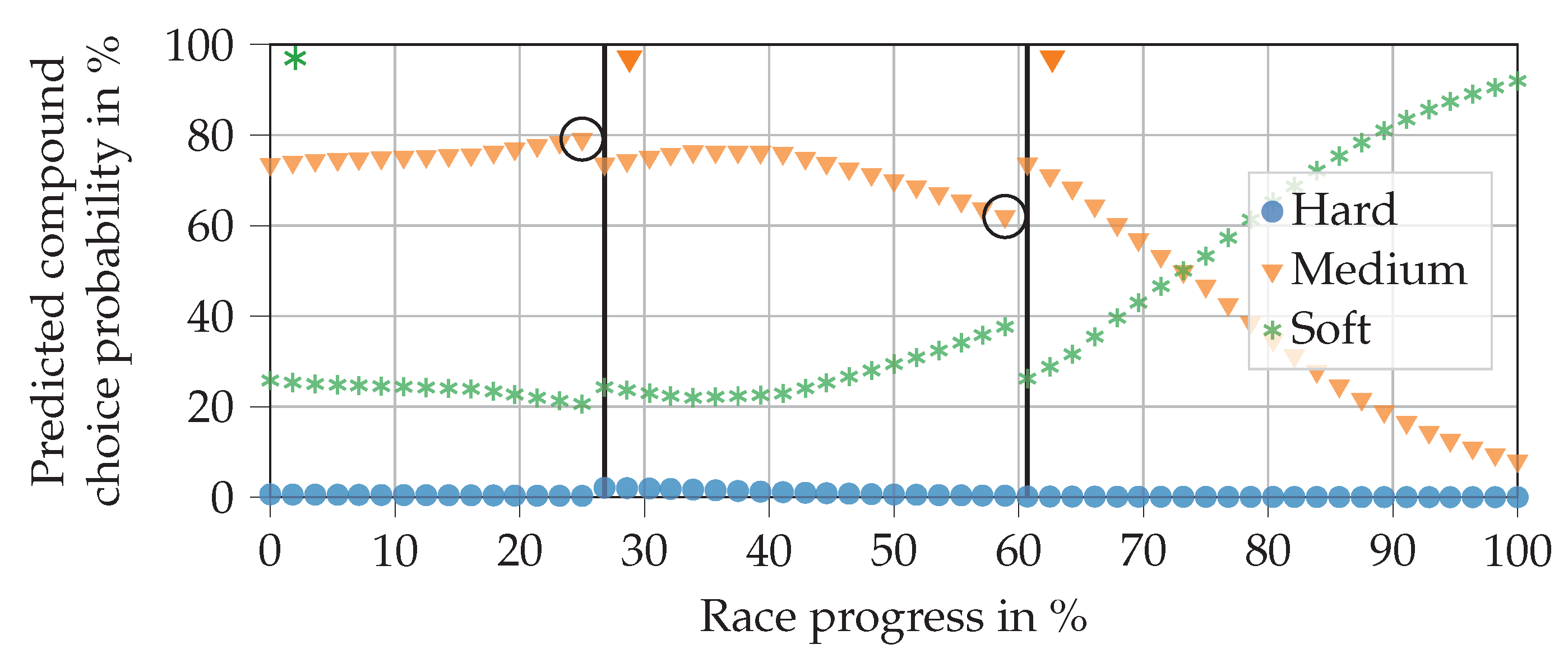
The progression of the curves are in line with expectations. In the first stint, the medium compound is more likely to be picked than the hard compound, since the NN knows that there are two stops remaining. It can also be seen that the attached soft compound has a probability of almost zero to be chosen. This happens to fulfill the rule that requires every driver to use two different compounds per race. Further analyses of various races and drivers showed that the NN meets this requirement consistently, presumably due to the remaining pit stops and fulfilled second compound features. At the beginning of the second stint, the hard compound has the highest probability (at a race progress of 30% to 40%). This would allow the driver to finish the race on the tires if he returned to the pits directly after the first stop. As the race progresses, the probability of choosing medium rises and falls until soft is the most likely choice. This is precisely where the second pit stop takes place. In the third stint, the remaining race progress is so small that it would only make sense to choose the soft compound again if another pit stop occurred.

If we have a race with only two available compounds (as in seasons 2014 and 2015), the NN’s hard compound output remains zero. Such a case is shown in Figure 13.

4.3.2. Analysis of Feature Impact

As before, we can analyze the behavior of the compound decision NN by varying single input features. Again, a 1-stop race was created with standard values, as shown in

Table 16. Standard values used to create the race for the feature impact analysis of the compound decision NN.

Feature	Standard Value
Race progress	$[0.0,1.0]$
Remaining pit stops	1
Relative compound	Soft
Race track	Austin
Fulfilled second compound	False
Number of avail. compounds	3

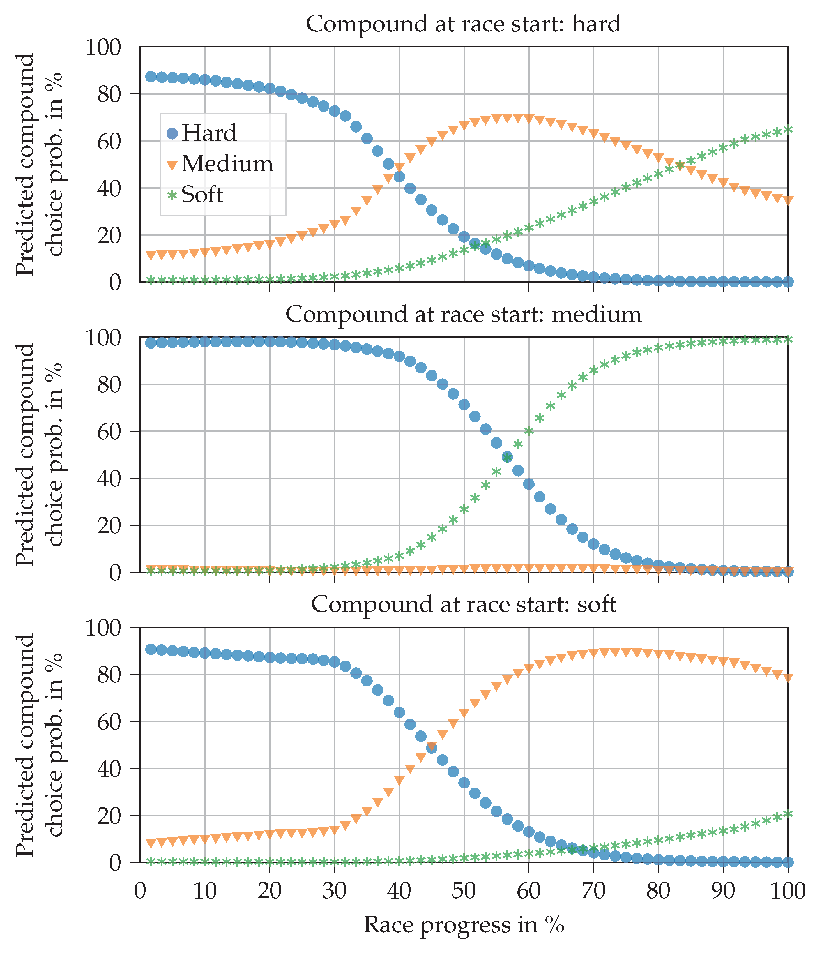
. The example analysis is shown in Figure 14.

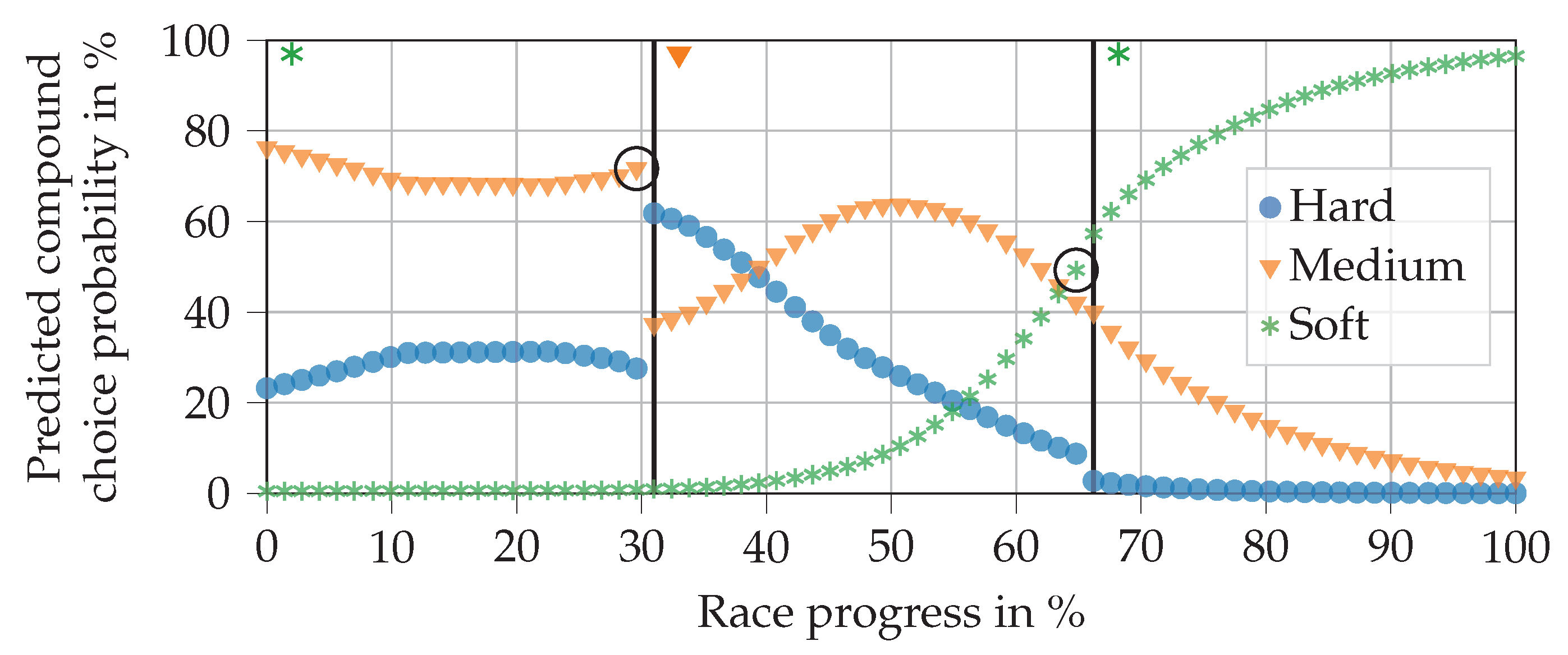
The top plot shows that during the first 40% of the race, the NN selects the hard compound, even though the hard compound is already fitted to the car and only a single pit stop is planned. This may appear unexpected at first but it can be explained. Firstly, most drivers begin the race with a soft or medium compound, which is why virtually no training data are available for a hard compound in the first stint, cp.

Table 17. Overview of tire compounds fitted at the race start. The values apply to data filtered according to Section 3.3.2.

Seasons	Start on Hard	Start on Medium	Start on Soft
≤2015	–	11.5%	88.5%
≥2016	4.4%	32.5%	63.1%
Overall	3.1%	26.0%	70.9%

. Secondly, if a driver starts with the hard compound, it is unlikely that he will change his tires before a race progress of 40%, especially if he is on a 1-stop strategy. Consequently, the first section of the prediction is not relevant, since the pit stop will usually take place in the middle of the race at the earliest.

The middle and bottom plots are in line with expectations. In the first part of the race, the NN chooses the hard compound. In the second part, it chooses either soft or medium, depending on the compound that is currently fitted to the car. Thus, the NN satisfies the regulations. It can also be seen that the soft compound is chosen above a race progress of 55% (middle plot), whereas the medium compound is selected above 45% (bottom plot). This is in line with the differences in durability between the two compounds.

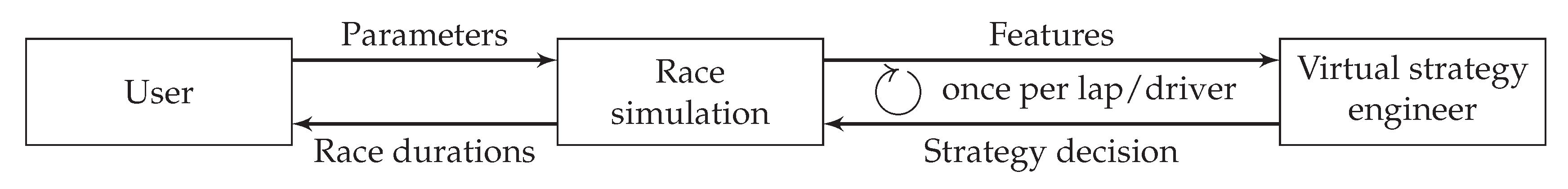
4.4. Integrating the Virtual Strategy Engineer into the Race Simulation

Figure 15 gives an overview of the integration of the VSE into the race simulation. As can be seen, the VSE is called once per lap and driver to make the strategy decision.

The race simulation is implemented in the Python programming language. One simulation run for an example race with 20 drivers and 55 laps takes about 100 $\mathrm{m}$$\mathrm{s}$ on a standard computer (Intel i7-6820HQ) if the strategy decisions are fixed. Since thousands of runs must be performed for Monte Carlo simulation, the time per run must remain in this magnitude, even if the VSE determines the participants’ strategies (although the runs are independent of each other and can be executed in parallel on CPUs with multiple cores). We could only achieve this by using TensorFlow Lite [51], a reduced framework whose original purpose is to bring ML functionality to devices such as mobile phones. Consequently, the trained models were converted into TensorFlow Lite models. Afterward, they only contain the functionality required for inferencing. This enables us to achieve calculation times of about 200 $\mathrm{m}$$\mathrm{s}$ per simulation run.

The race simulation allows us to compare the results when using different sources on which to base strategy decisions. For the analysis, we use simulation parameters that were fitted for the 2019 Austrian Grand Prix. The race is a good example because, in reality, there were no accidents or breakdowns, and therefore no FCY phases. Five variants of race strategy determination will be analyzed:

• Variant 1: All drivers use the strategy they have used in the real race
• Variant 2: Hamilton uses his optimized basic strategy, all other drivers use their real-race strategy
• Variant 3: The VSE determines Hamilton’s strategy, all other drivers use their real-race strategy
• Variant 4: The VSE determines Bottas’ strategy, all other drivers use their real-race strategy
• Variant 5: The VSE determines all drivers’ strategies

Hamilton and Bottas were chosen as test drivers because they achieve average result positions of $3.4$ and $3.8$ in the simulation with their real-race strategies, which allows the VSE to improve with different strategies. The real-race strategies of all drivers are given in

Table A2. Race strategies applied in the 2019 Austrian Grand Prix. The first lap with a new compound is stated in brackets. The real compound names are C2 (hard), C3 (medium), and C4 (soft). The drivers are listed in order of result position.

Driver	Strategy
Verstappen	Medium – hard (32)
Leclerc	Soft – hard (23)
Bottas	Medium – hard (22)
Vettel	Soft – hard (22) – soft (51)
Hamilton	Medium – hard (31)
Norris	Soft – Medium (26)
Gasly	Soft – hard (26)
Sainz	Medium – hard (42)
Räikkönen	Soft – hard (24)
Giovinazzi	Soft – hard (25)
Pérez	Medium – hard (29)
Ricciardo	Medium – soft (47)
Hülkenberg	Medium – hard (27)
Stroll	Medium – hard (26)
Albon	Medium – hard (36)
Grosjean	Medium – hard (35)
Kvyat	Medium – hard (33)
Russell	Medium – hard (28)
Magnussen	Soft – hard (12) – soft (63)
Kubica	Medium – hard (20)

, in the Appendix A. Hamilton’s basic strategy was determined as medium–medium (from lap 29)–soft (from lap 60) using the optimization algorithm presented. The VSE is based on the final trained NNs that were analyzed in Section 4.2.2 and Section 4.3.2.

We performed 10,000 simulation runs for each variant, which enabled us to make a reasonable estimate of the average result positions [3]. Probabilistic influences (lap time variability, race start performance, pit stop duration variability) were activated. FCY phases were deactivated for the first stage, to be added later. We furthermore deactivated retirements for all variants such that the result positions were based solely on racing and strategy decisions. The results of this first stage are shown in

Table 18. Real and average result positions of the top five drivers after 10,000 simulation runs of the 2019 Austrian Grand Prix. Five different variants of race strategy determination are compared. Probabilistic influences were activated, FCY phases were deactivated.

Driver	Real Race	Variant 1	Variant 2	Variant 3	Variant 4	Variant 5
Verstappen	1	1.2	1.2	1.2	1.2	1.0
Leclerc	2	2.0	2.1	2.2	2.0	2.5
Hamilton	5	3.4	3.1	2.9	3.4	3.6
Bottas	3	3.8	4.0	4.1	3.7	3.6
Vettel	4	5.7	5.7	5.7	5.9	7.4

. For simplicity, we display only the top five drivers of the simulated races.

First, it is noticeable that Hamilton’s result position in reality (five) differs strongly from that of the simulation with the real-race strategies ($3.4$ in Variant 1), which also causes large deviations for Bottas and Vettel. In the present case, this can be explained by the fact that Hamilton received a new front wing during his pit stop in reality, which increased the pit stop time loss by about 8 $\mathrm{s}$. This is not included in the simulation. In general, it must also be considered that a race simulation cannot perfectly reproduce a real race, for instance, because of model inaccuracies or parameterization errors. Furthermore, the progress of the race changes with different strategies. Consequently, the following results can only be compared with each other and not with a real-world race.

Hamilton achieves an average position of $3.4$ using his real strategy (Variant 1). By switching to the optimized basic strategy (Variant 2), this can be improved to $3.1$. This happens mainly at the expense of Bottas, who drops from $3.8$ to $4.0$. The VSE (Variant 3) results in further improvement to $2.9$. Using the VSE for Bottas has almost no impact on the average result position (Variant 4). If all drivers in the simulated race are led by the VSE (Variant 5), we can see that the result positions are quite different. Some drivers profit from the VSE decisions, e.g., Verstappen and Bottas, while others perform worse, e.g., Hamilton and Vettel.

In the second stage, we repeated the entire procedure with activated FCY phases. These are randomly generated according to [3]. The results are given in

Table 19. Real and average result positions of the top five drivers after 10,000 simulation runs of the 2019 Austrian Grand Prix. Five different variants of race strategy determination are compared. Both probabilistic influences and randomly generated FCY phases were activated.

Driver	Real Race	Variant 1	Variant 2	Variant 3	Variant 4	Variant 5
Verstappen	1	1.3	1.4	1.4	1.3	1.2
Leclerc	2	2.1	2.1	2.3	2.1	2.6
Hamilton	5	3.5	3.4	2.7	3.6	3.6
Bottas	3	3.9	4.0	4.1	3.5	3.6
Vettel	4	5.9	5.9	6.0	6.2	7.2

.

With activated FCY phases, we can see that the results are slightly worse than Variant 1 in the previous table. This is because FCY phases often allow drivers at the back to catch up with those at the front, which can involve overtaking maneuvers as soon as the phase is over. It is also evident that the basic strategy (Variant 2) improves Hamilton’s average result only slightly because it can hardly play out its optimality here (it was determined for a free track and without FCY phases). Variant 3 indicates that Hamilton benefits massively from the VSE that reacts to FCY phases in the simulation. His average result position improves to $2.7$. For Bottas, the VSE does not change that much, but it is still remarkable (Variant 4). Interestingly, in Variant 5, the results are quite similar to those of the first stage without FCY phases. This is in line with expectations, since the FCY phases do not change whether the VSE’s decision characteristics fit the corresponding driver parameterization well.

In conclusion, we can say that an optimized basic strategy can improve the results. However, this, of course, depends on the strategy used in comparison, as well as on the driver parameterization. Furthermore, the advantage disappears as soon as FCY phases are considered. The improvement that can be achieved by the VSE depends on whether the combination of decision characteristics and driver parameterization are compatible or not. In some cases, we also saw that the VSE worsens the result of the driver. However, particularly with FCY phases, the VSE often improves the result, due to its ability to react to the race situation.

5. Discussion

Starting with the simplest race simulation variant—a single driver on a free track with no probabilistic influences—an optimization problem can determine the fastest race strategy. The MIQP cannot only be used to set the remaining pit stops feature for the VSE, but also to obtain an initial strategic impression of a race. This is supported by fast computation times. On the downside, however, the optimization problem formulation is based on several assumptions from which the race can differ significantly. This includes the assumption of a free race track, as well as the assumption that the tire degradation can be described by a linear model and is independent of the changing vehicle mass. Furthermore, the optimization result is hugely dependent on the parameters of the tire degradation model. Consequently, the less these assumptions apply in a race, for instance, due to an FCY phase, the worse the basic strategy performs.

The VSE was developed to make automated race strategy decisions in a race simulation in all situations. We can conclude that, in general, it makes reasonable decisions and reacts consistently with the race situation, for instance, in the case of FCY phases or undercut attempts. Fast inference times make it suitable for use with any number of drivers, and its training on the entire database makes it universally applicable across all drivers, teams, and seasons. Using real-world data also prevents the VSE from learning modeling errors or parameterization errors, as might occur with reinforcement learning.

However, training on the entire database is also a disadvantage. Drivers, cars, and teams are subject to constant development, and the regulations change from season to season. This means that the VSE is not able to learn a ‘perfect’ reaction to specific situations. Training on real data is not ideal either, because even in real races, the strategy engineers sometimes make wrong decisions. Another aspect is the limited amount of data that is available to us, which also restricts the possible features. For example, an F1 team has a lot of sensor data at its disposal, which they use to determine the tire condition. However, from an external perspective, we cannot even distinguish reliably if the lap times of a driver deteriorate due to tire degradation or due to another engine mapping. Unfortunately, with the available data, we were also unable to create features that lead the VSE to make active use of advanced tactical opportunities such as undercuts. A possible feature that we did not consider is that pit stops are in reality, if possible, placed in such a way that the driver can drive freely afterward and is stuck behind other cars. Especially if sector times were available, this could help to improve the prediction quality. Another point is that in reality, strategic decisions are not only dependent on timing data, but also on game-theoretical factors. This is difficult to train, because we do not know which opponent(s) a driver was battling against in his race and what the expected results of all strategy combinations were that led to the subsequent decisions. When using the VSE in a race simulation, the method for specifying the intended number of pit stops could be improved. The current implementation based on the optimized basic strategy has the disadvantage that the number of pit stops is not adjusted, for example to the number of FCY phases.

Several points remain for future work. Firstly, merging the two stages of the current decision-making process into a single network could improve the prediction quality, since the NN would then consider the next tire compound for the pit stop decision. Secondly, with access to more detailed and extensive data, new features could be developed for improved predictions. A better representation of the tire state seems to be a good starting point. Thirdly, we believe that at the moment, a meaningful metric is missing to compare the characteristics of different race tracks objectively. Such a metric could be beneficial for both NNs to replace the race track and race track category features. A possible starting point could be the energy that is transferred via the tires per lap. Fourthly, the application and testing of the VSE in real-world races would enable a further evaluation of its decisions. However, since this will probably not be possible for us, we will focus on further analysis in simulation and comparison with the reinforcement learning approach currently under development.

6. Outlook: Reinforcement Learning Approach

Since we have no access to any team and are dependent on publicly available data, our future work will focus on a reinforcement learning approach. The race simulation will therefore be used as an environment for training an agent to make race strategy decisions. Here, as in real-world races, the agent can choose between four actions at the end of each lap: no pit stop, pit stop (hard), pit stop (medium), pit stop (soft). Thus, the decision is not divided into two stages, as in the methodology presented above. After rendering a decision, a lap is simulated under consideration of the chosen action. Before the agent chooses its next action, it is rewarded for its previous action, in two parts. The first part is determined by the difference between the current lap time and an average lap time calculated for the driver in a pre-simulation without opponents. Thus, the agent learns that it can increase its reward by fitting a fresh set of tires. The second part considers the number of positions that the driver has won or lost since the previous decision. Consequently, the agent will learn that a pit stop costs positions. By optimizing the strategy, the agent autonomously maximizes its reward.

In its current state, the agent is trained specifically for each race. During training, the other drivers’ strategies in the simulated race can be controlled by the VSE or be predefined by the user. To ensure that the agent can be used universally for all drivers and situations, the driver controlled during training is randomly selected before each training episode.

In initial tests, the agent achieved better results in the race simulation than the VSE. For the 2019 Chinese Grand Prix, in which there were 20 drivers, it achieved an average position of $8.46$ over 1000 simulated races, each with a randomly selected driver. The VSE only manages an average position of $9.51$. Various factors can explain the better performance of the agent. Firstly, the VSE is trained on many different real races and learns to make reasonable decisions ‘on average’, which may, however, not be a perfect fit for the driver, car, track, and race situation. The agent, in contrast, is trained specifically for the race in question. Secondly, the agent makes a pit stop decision in combination with the next compound, which enables better timing of the pit stop compared to the two-stage approach of the VSE. Thirdly, in contrast to the VSE, the agent does not need the intended number of pit stops for the race. This simplifies handling and allows him to amend the number of pit stops during the race if the situation changes.

The results of the initial tests seem promising, but must be evaluated in further races. Furthermore, we have to analyze whether the agent is able to learn and make active use of advanced tactical opportunities, such as the undercut. It is also necessary to check whether the agent’s strategies seem reasonable, since in training based purely on simulation, it will also learn the simulation and parameterization errors.

7. Summary

This paper presents a methodology for automating race strategy decisions in circuit motorsport. The focus is on the Formula 1 racing series and, thus, on the optimal determination of pit stops to replace worn-out tires. To be able to determine an initial estimate of the optimal race strategy, a quadratic optimization problem was set up that minimizes a driver’s race duration, assuming a race without opponents. However, this estimate is not sufficient to be used in a race simulation or a real-world race, as it takes neither the opponent drivers nor the particular race situation into account. Therefore, we developed a virtual strategy engineer (VSE) based on two artificial neural networks. The first one decides in each respective lap whether the driver should make a pit stop. If it chooses to call for a pit stop, a second neural network determines which of the available tire compounds should be fitted to the car. Both neural networks were trained on Formula 1 timing data of the seasons from 2014 to 2019. The presented results of a race simulation, in which the VSE is used to make the race strategy decisions, indicate that the VSE makes reasonable decisions and is able to adapt its strategy to the particular race situation. Thus, the VSE improves a race simulation’s realism and can support a real strategy engineer in his decisions.

The entire Python code for the race simulation, including the trained VSE models, is available under an open-source license on GitHub (https://github.com/TUMFTM/race-simulation).